Chapter 1: Functions
1.1 Functions and Their Graphs
Functions are a tool for describing the real world in mathematical terms. A function can be represented by an equation, a graph, a numerical table, or a verbal description; we will use all four representations throughout this text. This section reviews these ideas.
Functions; Domain and Range
The temperature at which water boils depends on the elevation above sea level. The interest paid on a cash investment depends on the length of time the investment is held. The area of a circle depends on the radius of the circle. The distance an object travels depends on the elapsed time.
In each case, the value of one variable quantity, say y, depends on the value of another variable quantity, which we often call x. We say that “y is a function of x” and write this symbolically as
The symbol f represents the function, the letter x is the independent variable representing the input value to f, and y is the dependent variable or output value of f at x.
DEFINITION A function f from a set D to a set Y is a rule that assigns a single value
in Y to each x in D. 𝑓 ( 𝑥 )
A rule that assigns more than one value to an input x, such as the rule that assigns to a positive number both the positive and negative square roots of the number, does not describe a function.
The set D of all possible input values is called the domain of the function. The domain of f will sometimes be denoted by
Often a function is given by a formula that describes how to calculate the output value from the input variable. For instance, the equation
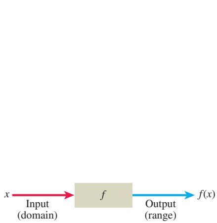
FIGURE 1.1 A diagram showing a function as a kind of machine.
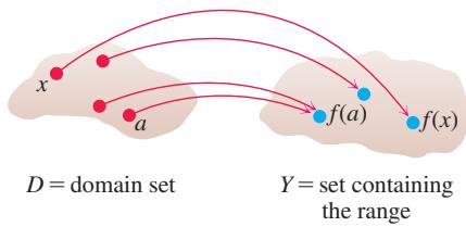
FIGURE 1.2 A function from a set D to a set Y assigns a unique element of Y to each element in D.
Changing the domain to which we apply a formula usually changes the range as well. The range of
When the range of a function is a set of real numbers, the function is said to be real-valued. The domains and ranges of most real-valued functions we consider are intervals or combinations of intervals. Sometimes the range of a function is not easy to find.
A function f is like a machine that produces an output value
A function can also be pictured as an arrow diagram (Figure 1.2). Each arrow associates to an element of the domain D a single element in the set Y. In Figure 1.2, the arrows indicate that
EXAMPLE 1 Verify the natural domains and associated ranges of some simple functions. The domains in each case are the values of x for which the formula makes sense.
| Function | Domain (x) | Range (y) |
Solution The formula
The formula
The formula
In
The formula
Graphs of Functions
If f is a function with domain D, its graph consists of the points in the Cartesian plane whose coordinates are the input-output pairs for f. In set notation, the graph is
The graph of the function
The graph of a function f is a useful picture of its behavior. If
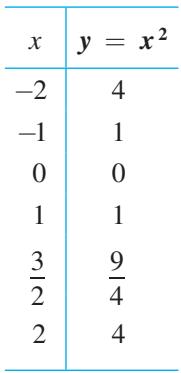
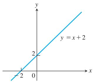
FIGURE 1.3 The graph of
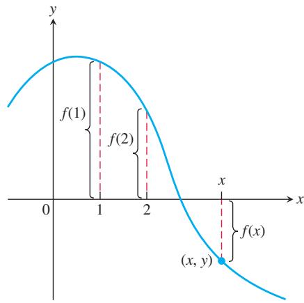
FIGURE 1.4 If
EXAMPLE 2 Graph the function
Solution Make a table of xy-pairs that satisfy the equation
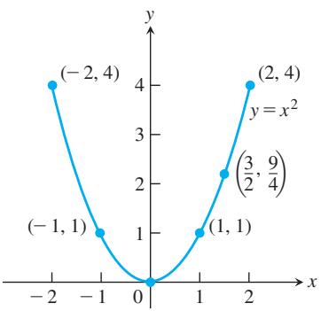
FIGURE 1.5 Graph of the function in Example 2.
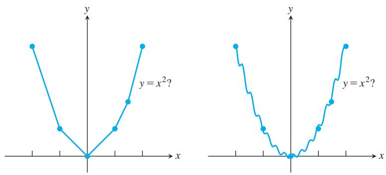
How do we know that the graph of
To find out, we could plot more points. But how would we then connect them? The basic question still remains: How do we know for sure what the graph looks like between the points we plot? Calculus answers this question, as we will see in Chapter 4. Meanwhile, we will have to settle for plotting points and connecting them as best we can.
| Time | Pressure |
| 0.00091 | -0.080 |
| 0.00108 | 0.200 |
| 0.00125 | 0.480 |
| 0.00144 | 0.693 |
| 0.00162 | 0.816 |
| 0.00180 | 0.844 |
| 0.00198 | 0.771 |
| 0.00216 | 0.603 |
| 0.00234 | 0.368 |
| 0.00253 | 0.099 |
| 0.00271 | -0.141 |
| 0.00289 | -0.309 |
| 0.00307 | -0.348 |
| 0.00325 | -0.248 |
| 0.00344 | -0.041 |
| 0.00362 | 0.217 |
| 0.00379 | 0.480 |
| 0.00398 | 0.681 |
| 0.00416 | 0.810 |
| 0.00435 | 0.827 |
| 0.00453 | 0.749 |
| 0.00471 | 0.581 |
| 0.00489 | 0.346 |
| 0.00507 | 0.077 |
| 0.00525 | -0.164 |
| 0.00543 | -0.320 |
| 0.00562 | -0.354 |
| 0.00579 | -0.248 |
| 0.00598 | -0.035 |
Representing a Function Numerically
A function may be represented algebraically by a formula and visually by a graph (Example 2). Another way to represent a function is numerically, through a table of values. From an appropriate table of values, a graph of the function can be obtained using the method illustrated in Example 2, possibly with the aid of a computer. The graph consisting of only the points in the table is called a scatterplot.
EXAMPLE 3 Musical notes are pressure waves in the air. The data associated with Figure 1.6 give recorded pressure displacement versus time in seconds of a musical note produced by a tuning fork. The table provides a representation of the pressure function (in micropascals) over time. If we first make a scatterplot and then draw a smooth curve that approximates the data points
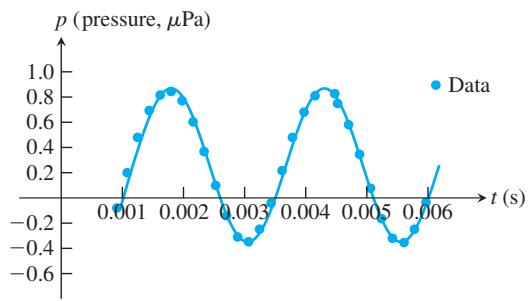
FIGURE 1.6 A smooth curve approximating the plotted points gives a graph of the pressure function represented by the accompanying tabled data (Example 3).
The Vertical Line Test for a Function
Not every curve in the coordinate plane can be the graph of a function. A function f can have only one value
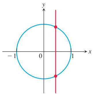
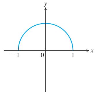
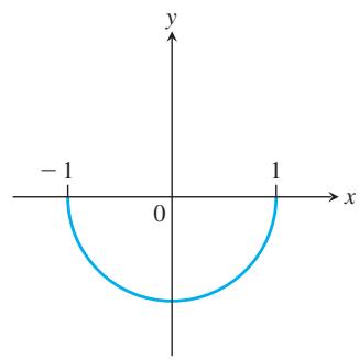
A circle cannot be the graph of a function, since some vertical lines intersect the circle twice. The circle graphed in Figure 1.7a, however, contains the graphs of two functions of x, namely the upper semicircle defined by the function
(a)
(b)
(c)
FIGURE 1.7 (a) The circle is not the graph of a function; it fails the vertical line test. (b) The upper semicircle is the graph of the function
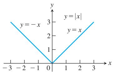
FIGURE 1.8 The absolute value function has domain
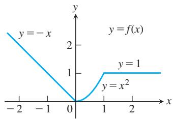
FIGURE 1.9 To graph the function
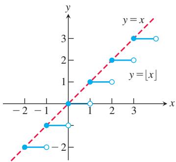
FIGURE 1.10 The graph of the greatest integer function
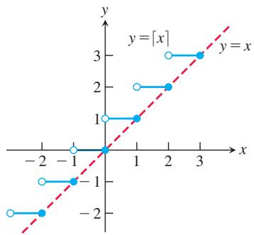
FIGURE 1.11 The graph of the least integer function
Piecewise-Defined Functions
Sometimes a function is described in pieces by using different formulas on different parts of its domain. One example is the absolute value function
whose graph is given in Figure 1.8. The right-hand side of the equation means that the function equals x if
EXAMPLE 4 The function
is defined on the entire real line but has values given by different formulas, depending on the position of x. The values of f are given by y = -x when x < 0,
EXAMPLE 5 The function whose value at any number x is the greatest integer less than or equal to x is called the greatest integer function or the integer floor function. It is denoted
EXAMPLE 6 The function whose value at any number x is the smallest integer greater than or equal to x is called the least integer function or the integer ceiling function. It is denoted [x]. Figure 1.11 shows the graph. For positive values of x, this function might represent, for example, the cost of parking x hours in a parking lot that charges $1 for each hour or part of an hour.
Increasing and Decreasing Functions
If the graph of a function climbs or rises as you move from left to right, we say that the function is increasing. If the graph descends or falls as you move from left to right, the function is decreasing.
DEFINITIONS Let f be a function defined on an interval I and let
and 𝑥 1 be two distinct points in I. 𝑥 2
If
whenever 𝑓 ( 𝑥 2 ) > 𝑓 ( 𝑥 1 ) , then f is said to be increasing on I. 𝑥 1 < 𝑥 2 If
whenever 𝑓 ( 𝑥 2 ) < 𝑓 ( 𝑥 1 ) , then f is said to be decreasing on I. 𝑥 1 < 𝑥 2
It is important to realize that the definitions of increasing and decreasing functions must be satisfied for every pair of points
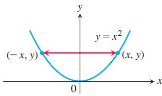
(a)
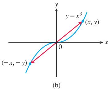
FIGURE 1.12 (a) The graph of
EXAMPLE 7 The function graphed in Figure 1.9 is decreasing on
Even Functions and Odd Functions: Symmetry
The graphs of even and odd functions have special symmetry properties.
DEFINITIONS A function
is an even function of 𝑦 = 𝑓 ( 𝑥 ) if 𝑥 , odd function of 𝑓 ( − 𝑥 ) = 𝑓 ( 𝑥 ) if 𝑥 , for every 𝑓 ( − 𝑥 ) = − 𝑓 ( 𝑥 ) in the function’s domain. 𝑥
The names even and odd come from powers of x. If y is an even power of x, as in
The graph of an even function is symmetric about the y-axis. Since
The graph of an odd function is symmetric about the origin. Since
Notice that each of these definitions requires that both x and -x be in the domain of f.
EXAMPLE 8 Here are several functions illustrating the definitions.
Even function:
Even function:
(a)
(b)
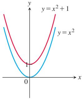
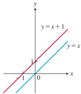
FIGURE 1.13 (a) When we add the constant term 1 to the function
Common Functions
A variety of important types of functions are frequently encountered in calculus.
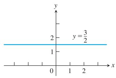
Linear Functions A function of the form
(b)
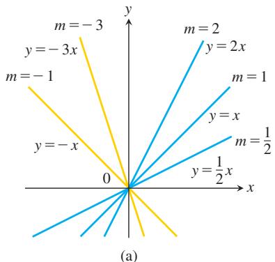
FIGURE 1.14 (a) Lines through the origin with slope m. (b) A constant function with slope m = 0.
DEFINITION Two variables y and x are proportional (to one another) if one is always a constant multiple of the other—that is, if y = kx for some nonzero constant k.
If the variable y is proportional to the reciprocal 1/x, then sometimes it is said that y is inversely proportional to x (because 1/x is the multiplicative inverse of x).
Power Functions A function
(a)
The graphs of

FIGURE 1.15 Graphs of
The graphs of the functions
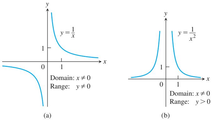
FIGURE 1.16 Graphs of the power functions
The functions
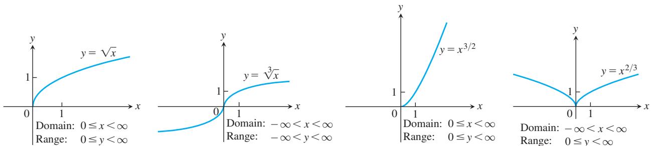
FIGURE 1.17 Graphs of the power functions
(b)
Polynomials A function p is a polynomial if
where n is a nonnegative integer and the numbers
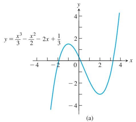
FIGURE 1.18 Graphs of three polynomial functions.
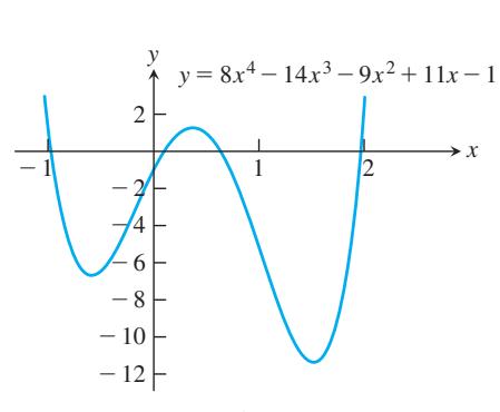
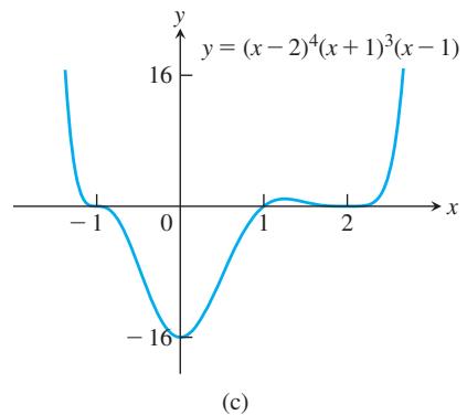
Rational Functions A rational function is a quotient or ratio
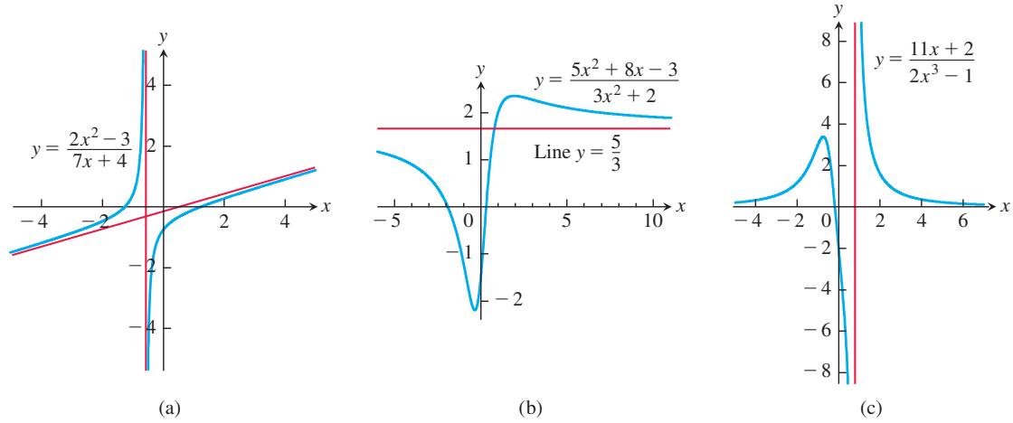
FIGURE 1.19 Graphs of three rational functions. The straight red lines approached by the graphs are called asymptotes and are not part of the graphs. We discuss asymptotes in Section 2.5.
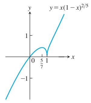
Algebraic Functions Any function constructed from polynomials using algebraic operations (addition, subtraction, multiplication, division, and taking roots) lies within the class of algebraic functions. All rational functions are algebraic, but also included are more complicated functions (such as those satisfying an equation like
(b)
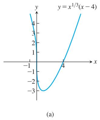
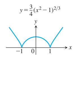
FIGURE 1.20 Graphs of three algebraic functions.
Trigonometric Functions The six basic trigonometric functions are reviewed in Section 1.3. The graphs of the sine and cosine functions are shown in Figure 1.21.
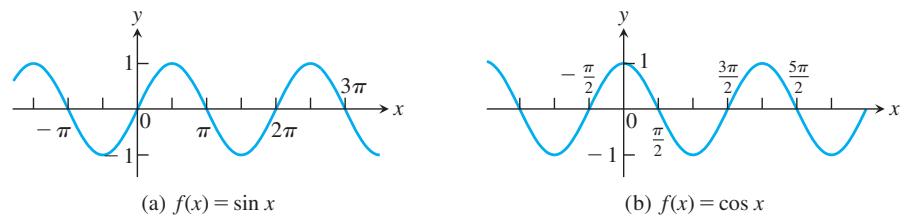
FIGURE 1.21 Graphs of the sine and cosine functions.
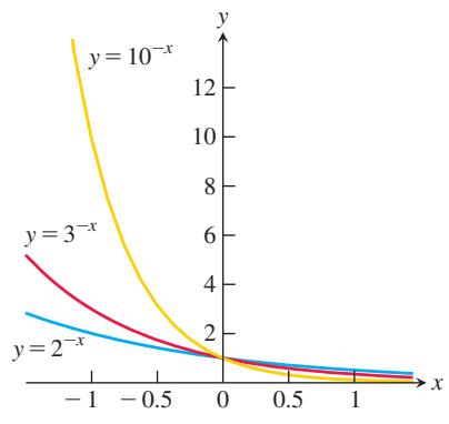
Exponential Functions A function of the form
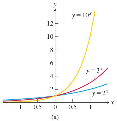
FIGURE 1.22 Graphs of exponential functions.
Logarithmic Functions These are the functions
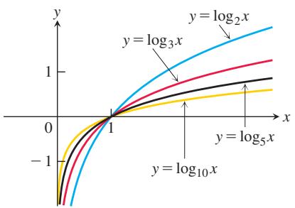
FIGURE 1.23 Graphs of four logarithmic functions.
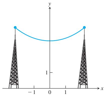
FIGURE 1.24 Graph of a catenary or hanging cable. (The Latin word catena means “chain.”)
Transcendental Functions These are functions that are not algebraic. They include the trigonometric, inverse trigonometric, exponential, and logarithmic functions, and many other functions as well. The catenary is one example of a transcendental function. Its graph has the shape of a cable, like a telephone line or electric cable, strung from one support to another and hanging freely under its own weight (Figure 1.24). The function defining the graph is discussed in Section 7.3.
Exercises 1.1
Functions
In Exercises 1–6, find the domain and range of each function.
-
𝑓 ( 𝑥 ) = 1 + 𝑥 2 -
𝑓 ( 𝑥 ) = 1 − √ 𝑥 -
𝐹 ( 𝑥 ) = √ 5 𝑥 + 1 0 -
𝑔 ( 𝑥 ) = √ 𝑥 2 − 3 𝑥 -
𝑓 ( 𝑡 ) = 4 3 − 𝑡 -
𝐺 ( 𝑡 ) = 2 𝑡 2 − 1 6
In Exercises 7 and 8, which of the graphs are graphs of functions of
- a.
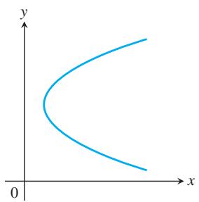
b.
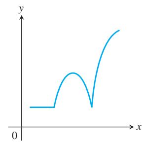
- a.
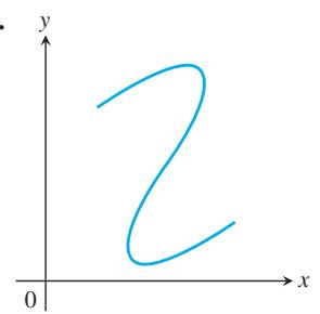
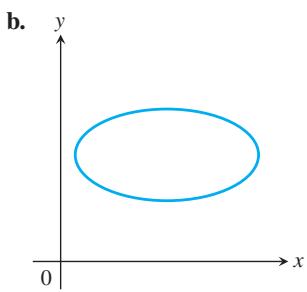
Finding Formulas for Functions
-
Express the area and perimeter of an equilateral triangle as a function of the triangle’s side length
𝑥 -
Express the side length of a square as a function of the length
𝑑 -
Express the edge length of a cube as a function of the cube’s diagonal length
𝑑 -
A point P in the first quadrant lies on the graph of the function
𝑓 ( 𝑥 ) = √ 𝑥 -
Consider the point
( 𝑥 , 𝑦 ) 2 𝑥 + 4 𝑦 = 5 ( 𝑥 , 𝑦 ) ( 0 , 0 ) -
Consider the point
( 𝑥 , 𝑦 ) 𝑦 = √ 𝑥 − 3 ( 𝑥 , 𝑦 ) ( 4 , 0 )
Functions and Graphs
Find the natural domain and graph the functions in Exercises 15-20.
-
𝑓 ( 𝑥 ) = 5 − 2 𝑥 -
𝑓 ( 𝑥 ) = 1 − 2 𝑥 − 𝑥 2 -
𝑔 ( 𝑥 ) = √ | 𝑥 | -
𝑔 ( 𝑥 ) = √ − 𝑥 -
𝐹 ( 𝑡 ) = 𝑡 / | 𝑡 | -
𝐺 ( 𝑡 ) = 1 / | 𝑡 | -
Find the domain of
𝑦 = 𝑥 + 3 4 − √ 𝑥 2 − 9 -
Find the range of
𝑦 = 2 + √ 9 + 𝑥 2 -
Graph the following equations and explain why they are not graphs of functions of
𝑥
a.
b.
- Graph the following equations and explain why they are not graphs of functions of
𝑥
a.
b.
Piecewise-Defined Functions
Graph the functions in Exercises 25–28.
-
𝑓 ( 𝑥 ) = { 𝑥 , 0 ≤ 𝑥 ≤ 1 2 − 𝑥 , 1 < 𝑥 ≤ 2 -
𝑔 ( 𝑥 ) = { 1 − 𝑥 , 0 ≤ 𝑥 ≤ 1 2 − 𝑥 , 1 < 𝑥 ≤ 2 -
𝐹 ( 𝑥 ) = { 4 − 𝑥 2 , 𝑥 ≤ 1 𝑥 2 + 2 𝑥 , 𝑥 > 1 -
𝐺 ( 𝑥 ) = { 1 / 𝑥 , 𝑥 < 0 𝑥 , 0 ≤ 𝑥
Find a formula for each function graphed in Exercises 29-32.
- a.
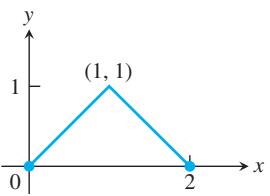
b.
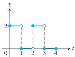
- a.
b.
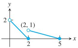
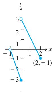
- a.
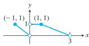
b.
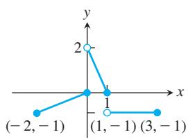
- a.
b.
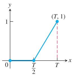
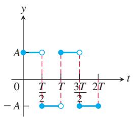
The Greatest and Least Integer Functions
- For what values of
𝑥
a.
b.
-
What real numbers
𝑥 ⌊ 𝑥 ⌋ = ⌈ 𝑥 ⌉ -
Does
⌈ − 𝑥 ⌉ = − ⌊ 𝑥 ⌋ -
Graph the function
Why is
Increasing and Decreasing Functions
Graph the functions in Exercises 37–46. What symmetries, if any, do the graphs have? Specify the intervals over which the function is increasing and the intervals where it is decreasing.
-
𝑦 = − 𝑥 3 -
𝑦 = − 1 𝑥 2 -
𝑦 = − 1 𝑥 -
𝑦 = 1 | 𝑥 | -
𝑦 = √ | 𝑥 | -
𝑦 = √ − 𝑥 -
𝑦 = 𝑥 3 / 8 -
𝑦 = − 4 √ 𝑥 -
𝑦 = − 𝑥 3 / 2 -
𝑦 = ( − 𝑥 ) 2 / 3
Even and Odd Functions
In Exercises 47–62, say whether the function is even, odd, or neither. Give reasons for your answer.
-
𝑓 ( 𝑥 ) = 3 -
𝑓 ( 𝑥 ) = 𝑥 − 5 -
𝑓 ( 𝑥 ) = 𝑥 2 + 1 -
𝑓 ( 𝑥 ) = 𝑥 2 + 𝑥 -
𝑔 ( 𝑥 ) = 𝑥 3 + 𝑥 -
𝑔 ( 𝑥 ) = 𝑥 4 + 3 𝑥 2 − 1 -
𝑔 ( 𝑥 ) = 1 𝑥 2 − 1 -
𝑔 ( 𝑥 ) = 𝑥 𝑥 2 − 1 -
ℎ ( 𝑡 ) = 1 𝑡 − 1 -
ℎ ( 𝑡 ) = | 𝑡 3 | -
ℎ ( 𝑡 ) = 2 𝑡 + 1 -
ℎ ( 𝑡 ) = 2 | 𝑡 | + 1 -
sin 2x
-
s i n 𝑥 2 -
cos 3x
-
1 + c o s 𝑥
Theory and Examples
-
The variable s is proportional to t, and s = 25 when t = 75. Determine t when s = 60.
-
Kinetic energy The kinetic energy K of a mass is proportional to the square of its velocity v. If K = 12,960 joules when v = 18 m/s, what is K when v = 10 m/s?
-
The variables r and s are inversely proportional, and r = 6 when s = 4. Determine s when r = 10.
-
Boyle’s law Boyle’s law says that the volume
𝑉 𝑃 𝑉 𝑃 𝑃 = 1 4 . 7 N / c m 2 𝑉 = 1 0 0 0 c m 3 𝑉 𝑃 = 2 3 . 4 N / c m 2 -
A box with an open top is to be constructed from a rectangular piece of cardboard with dimensions 14 cm by 22 cm by cutting out equal squares of side x at each corner and then folding up the sides as in the figure. Express the volume V of the box as a function of x.
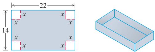
- The accompanying figure shows a rectangle inscribed in an isosceles right triangle whose hypotenuse is 2 units long.
a. Express the y-coordinate of P in terms of x. (You might start by writing an equation for the line AB.)
b. Express the area of the rectangle in terms of x.
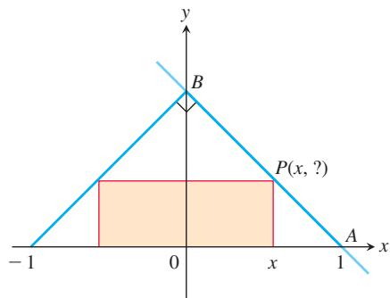
In Exercises 69 and 70, match each equation with its graph. Do not use a graphing device, and give reasons for your answer.
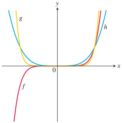
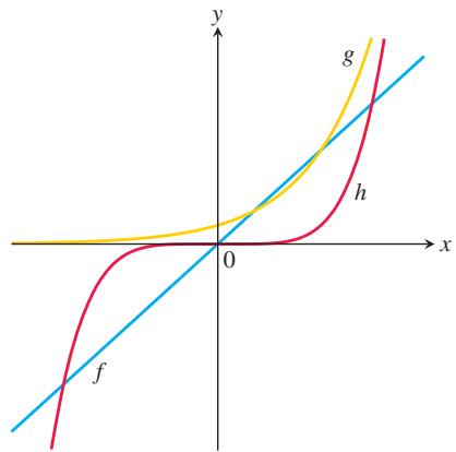
T 71. a. Graph the functions
b. Confirm your findings in part (a) algebraically.
T 72. a. Graph the functions
b. Confirm your findings in part (a) algebraically.
-
For a curve to be symmetric about the x-axis, the point
( 𝑥 , 𝑦 ) ( 𝑥 , − 𝑦 ) -
Three hundred books sell for
4 0 𝑒 𝑎 𝑐 ℎ , 𝑟 𝑒 𝑠 𝑢 𝑙 𝑡 𝑖 𝑛 𝑔 𝑖 𝑛 𝑎 𝑟 𝑒 𝑣 𝑒 𝑛 𝑢 𝑒 𝑜 𝑓 4 0 ) = . 𝐹 𝑜 𝑟 𝑒 𝑎 𝑐 ℎ -
A pen in the shape of an isosceles right triangle with legs of length x m and hypotenuse of length h m is to be built. If fencing costs
5 / 𝑚 𝑓 𝑜 𝑟 𝑡 ℎ 𝑒 𝑙 𝑒 𝑔 𝑠 𝑎 𝑛 𝑑 -
Industrial costs A power plant sits next to a river where the river is 250 m wide. To lay a new cable from the plant to a location in the city 2 km downstream on the opposite side costs
1 8 0 𝑝 𝑒 𝑟 𝑚 𝑒 𝑡 𝑒 𝑟 𝑎 𝑐 𝑟 𝑜 𝑠 𝑠 𝑡 ℎ 𝑒 𝑟 𝑖 𝑣 𝑒 𝑟 𝑎 𝑛 𝑑
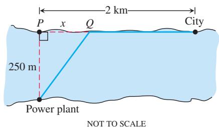
NOT TO SCALE
a. Suppose that the cable goes from the plant to a point Q on the opposite side that is x m from the point P directly opposite the plant. Write a function
b. Generate a table of values to determine if the least expensive location for point Q is less than 300 m or greater than 300 m from point P.
1.2 Combining Functions; Shifting and Scaling Graphs
In this section we look at the main ways functions are combined or transformed to form new functions.
Sums, Differences, Products, and Quotients
Like numbers, functions can be added, subtracted, multiplied, and divided (except where the denominator is zero) to produce new functions. If f and g are functions, then for every x that belongs to the domains of both f and g (that is, for
Notice that the + sign on the left-hand side of the first equation represents the operation of addition of functions, whereas the + on the right-hand side of the equation means addition of the real numbers
At any point of
Functions can also be multiplied by constants: If
EXAMPLE 1 The functions defined by the formulas
have domains
The following table summarizes the formulas and domains for the various algebraic combinations of the two functions. We also write
| Function | Formula | Domain |
The graph of the function
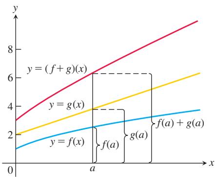
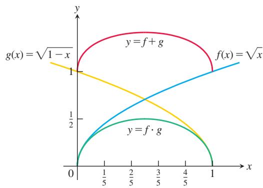
FIGURE 1.25 Graphical addition of two functions.
FIGURE 1.26 The domain of the function
Composing Functions
Composition is another method for combining functions. In this operation the output from one function becomes the input to a second function.
DEFINITION If f and g are functions, the function
(“f composed with g”) is defined by 𝑓 ∘ 𝑔 ( 𝑓 ∘ 𝑔 ) ( 𝑥 ) = 𝑓 ( 𝑔 ( 𝑥 ) ) and called the composition of
and 𝑓 . The domain of 𝑔 consists of the numbers 𝑓 ∘ 𝑔 in the domain of 𝑥 for which 𝑔 lies in the domain of 𝑔 ( 𝑥 ) . 𝑓
To find
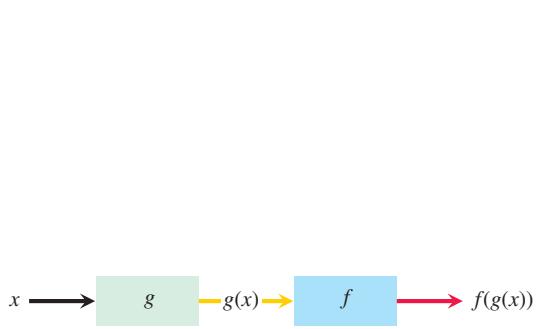
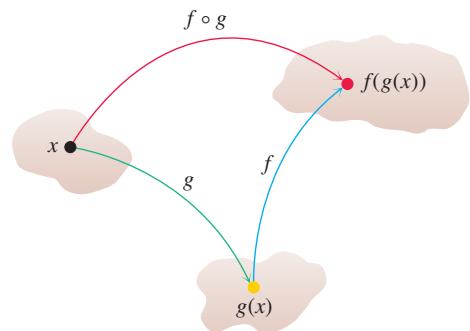
FIGURE 1.27 The composition
FIGURE 1.28 Arrow diagram for
To evaluate the composition
The functions
EXAMPLE 2 If
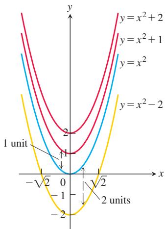
FIGURE 1.29 To shift the graph of
(a)
Solution
Composition
Domain
To see why the domain of
Notice that if
Shifting a Graph of a Function
A common way to obtain a new function from an existing one is by adding a constant to each output of the existing function, or to its input variable. The graph of the new function is the graph of the original function shifted vertically or horizontally, as follows.
Shift Formulas
Vertical Shifts
Shifts it down
Horizontal Shifts
Shifts it right |h| units if h < 0
EXAMPLE 3
(a) Adding 1 to the right-hand side of the formula
(b) Adding
(c) Adding 3 to x in
(d) Adding
Scaling and Reflecting a Graph of a Function
To scale the graph of a function
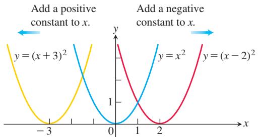
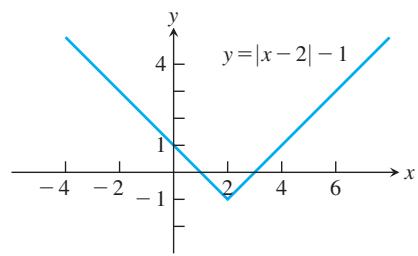
FIGURE 1.30 To shift the graph of
FIGURE 1.31 The graph of
Vertical and Horizontal Scaling and Reflecting Formulas
For c > 1, the graph is scaled:
EXAMPLE 4 Here we scale and reflect the graph of
(a) Vertical: Multiplying the right-hand side of
(b) Horizontal: The graph of
(c) Reflection: The graph of
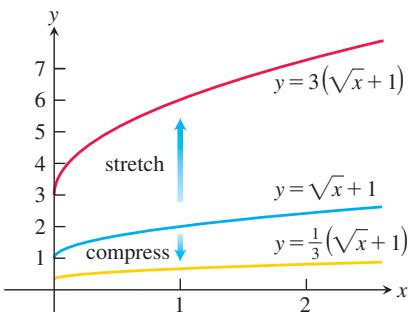
FIGURE 1.32 Vertically stretching and compressing the graph of
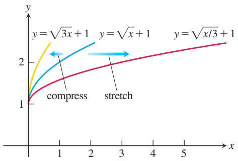
FIGURE 1.33 Horizontally stretching and compressing the graph of
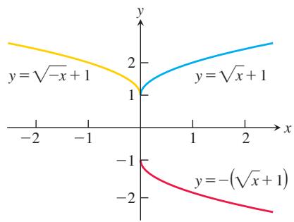
FIGURE 1.34 Reflections of the graph of
EXAMPLE 5 Given the function
(a) horizontal compression by a factor of 2 followed by reflection across the y-axis (Figure 1.35b).
(b) vertical compression by a factor of 2 followed by reflection across the x-axis (Figure 1.35c).
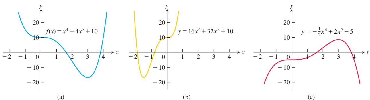
FIGURE 1.35 (a) The original graph of f. (b) The horizontal compression of
Solution
(a) We multiply
(b) The formula is
EXERCISES
Algebraic Combinations
In Exercises 1 and 2, find the domains of
-
𝑓 ( 𝑥 ) = 𝑥 , 𝑔 ( 𝑥 ) = √ 𝑥 − 1 -
𝑓 ( 𝑥 ) = √ 𝑥 + 1 𝑔 ( 𝑥 ) = √ 𝑥 − 1
In Exercises 3 and 4, find the domains of
-
𝑓 ( 𝑥 ) = 2 , 𝑔 ( 𝑥 ) = 𝑥 2 + 1 -
𝑓 ( 𝑥 ) = 1 , 𝑔 ( 𝑥 ) = 1 + √ 𝑥
Compositions of Functions
- If
𝑓 ( 𝑥 ) = 𝑥 + 5 𝑔 ( 𝑥 ) = 𝑥 2 − 3
b.
a.
c.
d.
e.
f.
g.
- If
𝑓 ( 𝑥 ) = 𝑥 − 1 𝑔 ( 𝑥 ) = 1 / ( 𝑥 + 1 )
a.
c.
e.
g.
In Exercises 7–10, write a formula for
-
𝑓 ( 𝑥 ) = 𝑥 + 1 , 𝑔 ( 𝑥 ) = 3 𝑥 , ℎ ( 𝑥 ) = 4 − 𝑥 -
𝑓 ( 𝑥 ) = 3 𝑥 + 4 , 𝑔 ( 𝑥 ) = 2 𝑥 − 1 , ℎ ( 𝑥 ) = 𝑥 2 -
𝑓 ( 𝑥 ) = √ 𝑥 + 1 , 𝑔 ( 𝑥 ) = 1 𝑥 + 4 , ℎ ( 𝑥 ) = 1 𝑥 -
𝑓 ( 𝑥 ) = 𝑥 + 2 3 − 𝑥 , 𝑔 ( 𝑥 ) = 𝑥 2 𝑥 2 + 1 , ℎ ( 𝑥 ) = √ 2 − 𝑥
Let
- a.
𝑦 = √ 𝑥 − 3
b.
d.
- a.
𝑦 = 2 𝑥 − 3
b.
e.
f.
- Copy and complete the following table.
| a. | ? | ||
| b. | ? | ||
| c. | ? | ||
| d. | ? | ||
| e. | ? | ||
| f. | ? |
- Copy and complete the following table.
| g(x) | f(x) | ||
| a. | ? | ||
| b. | ? | ||
| c. | ? | ||
| d. | ? |
- Evaluate each expression using the given table of values:
| x | -2 | -1 | 0 | 1 | 2 |
| f(x) | 1 | 0 | -2 | 1 | 2 |
| g(x) | 2 | 1 | 0 | -1 | 0 |
a.
c.
e.
- Evaluate each expression using the functions
a.
d.
In Exercises 17 and 18, (a) write formulas for
-
𝑓 ( 𝑥 ) = √ 𝑥 + 1 , 𝑔 ( 𝑥 ) = 1 𝑥 -
𝑓 ( 𝑥 ) = 𝑥 2 , 𝑔 ( 𝑥 ) = 1 − √ 𝑥 -
Let
𝑓 ( 𝑥 ) = 𝑥 𝑥 − 2 𝑦 = 𝑔 ( 𝑥 ) ( 𝑓 ∘ 𝑔 ) ( 𝑥 ) = 𝑥 -
Let
𝑓 ( 𝑥 ) = 2 𝑥 3 − 4 𝑦 = 𝑔 ( 𝑥 ) ( 𝑓 ∘ 𝑔 ) ( 𝑥 ) = 𝑥 + 2 -
A balloon’s volume
𝑉 𝑉 = 𝑠 2 + 2 𝑠 + 3 c m 3 𝑠 ∘ C 𝑠 𝑡 𝑠 = 2 𝑡 − 3 ∘ C 𝑉 𝑡 -
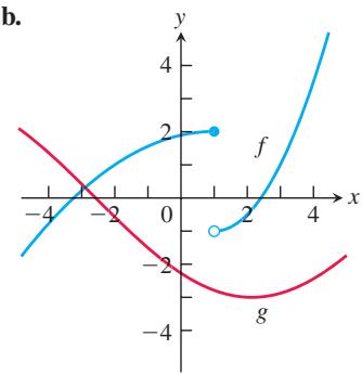
Use the graphs of
𝑓 𝑔 𝑦 = 𝑓 ( 𝑔 ( 𝑥 ) )
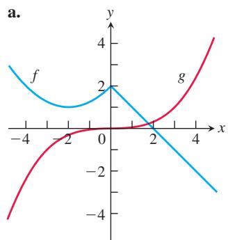
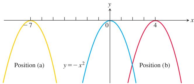
Shifting Graphs
- The accompanying figure shows the graph of
𝑦 = − 𝑥 2
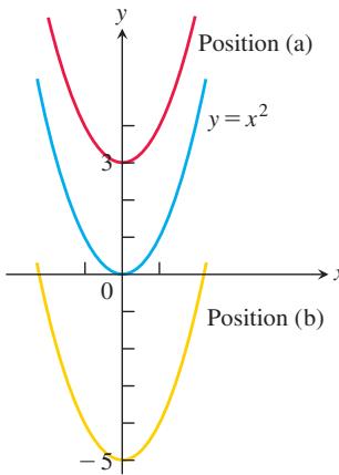
- The accompanying figure shows the graph of
𝑦 = 𝑥 2
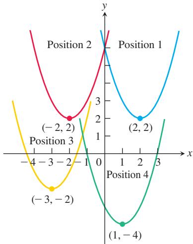
- Match the equations listed in parts (a)-(d) to the graphs in the accompanying figure.
a.
b.
c.
d.
- The accompanying figure shows the graph of
𝑦 = − 𝑥 2
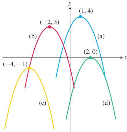
Exercises 27–36 tell how many units and in what directions the graphs of the given equations are to be shifted. Give an equation for the shifted graph. Then sketch the original and shifted graphs together, labeling each graph with its equation.
-
𝑥 2 + 𝑦 2 = 4 9 -
𝑥 2 + 𝑦 2 = 2 5 -
𝑦 = 𝑥 3 -
𝑦 = 𝑥 2 / 3 -
𝑦 = √ 𝑥 -
𝑦 = − √ 𝑥 -
𝑦 = 2 𝑥 − 7 -
𝑦 = 1 2 ( 𝑥 + 1 ) + 5 -
𝑦 = 1 / 𝑥 -
𝑦 = 1 / 𝑥 2
Graph the functions in Exercises 37–56.
-
𝑦 = √ 𝑥 + 4 -
𝑦 = √ 9 − 𝑥 -
𝑦 = | 𝑥 − 2 | -
𝑦 = | 1 − 𝑥 | − 1 -
𝑦 = 1 + √ 𝑥 − 1 -
𝑦 = 1 − √ 𝑥 -
𝑦 = ( 𝑥 + 1 ) 2 / 3 -
𝑦 = ( 𝑥 − 8 ) 2 / 3 -
𝑦 = 1 − 𝑥 2 / 3 -
𝑦 + 4 = 𝑥 2 / 3 -
𝑦 = 3 √ 𝑥 − 1 − 1 -
𝑦 = ( 𝑥 + 2 ) 3 / 2 + 1 -
𝑦 = 1 𝑥 − 2 -
𝑦 = 1 𝑥 − 2 -
𝑦 = 1 𝑥 + 2 -
𝑦 = 1 𝑥 + 2 -
𝑦 = 1 ( 𝑥 − 1 ) 2 -
𝑦 = 1 𝑥 2 − 1 -
𝑦 = 1 𝑥 2 + 1 -
𝑦 = 1 ( 𝑥 + 1 ) 2 -
The accompanying figure shows the graph of a function
𝑓 ( 𝑥 )
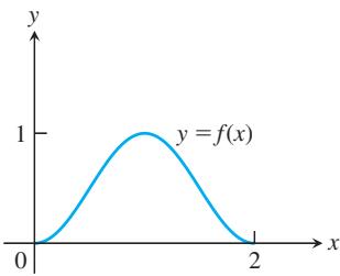
a.
c.
e.
g.
- The accompanying figure shows the graph of a function
𝑔 ( 𝑡 ) [ − 4 , 0 ] [ − 3 , 0 ]
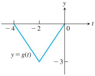
a.
b.
c.
d.
e.
f.
g.
h.
Vertical and Horizontal Scaling
Exercises 59–68 tell in what direction and by what factor the graphs of the given functions are to be stretched or compressed. Give an equation for the stretched or compressed graph.
-
𝑦 = 𝑥 2 − 1 -
𝑦 = 𝑥 2 − 1 -
𝑦 = 1 + 1 𝑥 2 -
𝑦 = 1 + 1 𝑥 2 -
𝑦 = √ 𝑥 + 1 -
𝑦 = √ 𝑥 + 1 -
𝑦 = √ 4 − 𝑥 2 -
𝑦 = √ 4 − 𝑥 2 -
𝑦 = 1 − 𝑥 3 -
𝑦 = 1 − 𝑥 3
Graphing
In Exercises 69–76, graph each function not by plotting points, but by starting with the graph of one of the standard functions presented in Figures 1.14–1.17 and applying an appropriate transformation.
-
𝑦 = − √ 2 𝑥 + 1 -
𝑦 = √ 1 − 𝑥 2 -
𝑦 = ( 𝑥 − 1 ) 3 + 2 -
𝑦 = ( 1 − 𝑥 ) 3 + 2 -
𝑦 = 1 2 𝑥 − 1 -
𝑦 = 2 𝑥 2 + 1 -
𝑦 = − 3 √ 𝑥 -
𝑦 = ( − 2 𝑥 ) 2 / 3 -
Graph the function
𝑦 = | 𝑥 2 − 1 | -
Graph the function
𝑦 = √ | 𝑥 |
Combining Functions
- Assume that
𝑓 𝑔 𝑓 𝑔 ( − ∞ , ∞ )
b. f/g
c. g/f
d.
e.
f.
g.
h.
i.
-
Can a function be both even and odd? Give reasons for your answer.
-
(Continuation of Example 1.) Graph the functions
𝑓 ( 𝑥 ) = √ 𝑥 𝑔 ( 𝑥 ) = √ 1 − 𝑥
T 82. Let
1.3 Trigonometric Functions
Angles
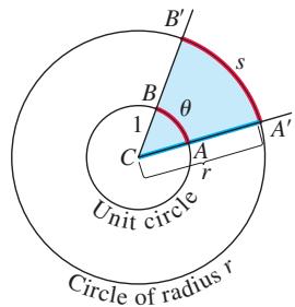
FIGURE 1.36 The radian measure of the central angle
and
This section reviews radian measure and the basic trigonometric functions.
Angles are measured in degrees or radians. The number of radians in the central angle
If the circle is a unit circle having radius r = 1, then from Figure 1.36 and Equation (1), we see that the central angle
Table 1.1 shows the equivalence between degree and radian measures for some basic angles.
TABLE 1.1 Angles measured in degrees and radians
| Degrees | -180 | -135 | -90 | -45 | 0 | 30 | 45 | 60 | 90 | 120 | 135 | 150 | 180 | 270 | 360 |
| θ (radians) | -π | 0 |
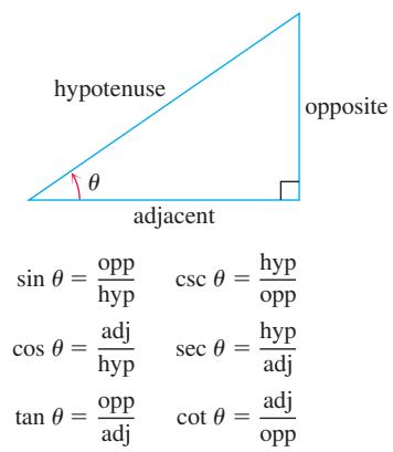
FIGURE 1.39 Trigonometric ratios of an acute angle.
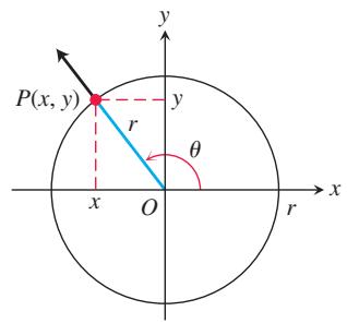
FIGURE 1.40 The trigonometric functions of a general angle
An angle in the xy-plane is said to be in standard position if its vertex lies at the origin and its initial ray lies along the positive x-axis (Figure 1.37). Angles measured counterclockwise from the positive x-axis are assigned positive measures; angles measured clockwise are assigned negative measures.
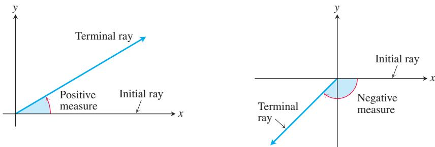
FIGURE 1.37 Angles in standard position in the xy-plane.
Angles describing counterclockwise rotations can go arbitrarily far beyond
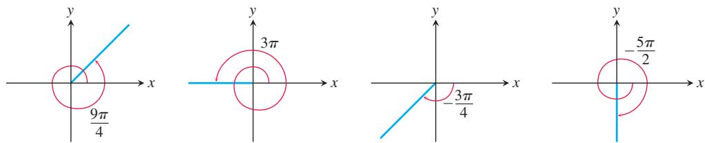
FIGURE 1.38 Nonzero radian measures can be positive or negative and can go beyond
Angle Convention: Use Radians From now on in this text, it is assumed that all angles are measured in radians unless degrees or some other unit is stated explicitly. When we talk about the angle
The Six Basic Trigonometric Functions
The trigonometric functions of an acute angle are given in terms of the sides of a right triangle (Figure 1.39). We extend this definition to obtuse and negative angles by first placing the angle in standard position in a circle of radius
sine:
cosine:
cosecant:
tangent:
secant:
cotangent:
These extended definitions agree with the right-triangle definitions when the angle is acute.
Notice also that whenever the quotients are defined,
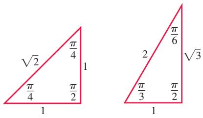
FIGURE 1.41 Radian angles and side lengths of two common triangles.
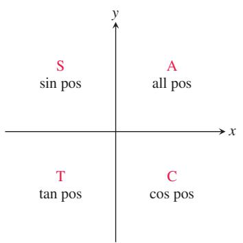
FIGURE 1.42 The ASTC rule, remembered by the statement “All Students Take Calculus,” tells which trigonometric functions are positive in each quadrant.
As you can see,
The exact values of these trigonometric ratios for some angles can be read from the triangles in Figure 1.41. For instance,
The ASTC rule (Figure 1.42) is useful for remembering when the basic trigonometric functions are positive or negative. For instance, from the triangle in Figure 1.43, we see that
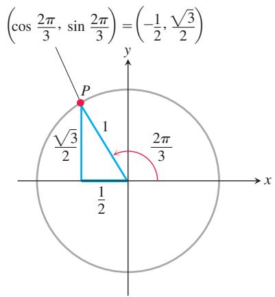
FIGURE 1.43 The triangle for calculating the sine and cosine of
Using a similar method we obtain the values of
TABLE 1.2 Values of sin θ, cos θ, and tan θ for selected values of θ
| Degrees | -180 | -135 | -90 | -45 | 0 | 30 | 45 | 60 | 90 | 120 | 135 | 150 | 180 | 270 | 360 |
| θ (radians) | -π | 0 | π | ||||||||||||
| sin θ | 0 | -1 | 0 | 1 | 0 | -1 | 0 | ||||||||
| cos θ | -1 | 0 | 1 | 0 | -1 | 0 | 1 | ||||||||
| tan θ | 0 | 1 | -1 | 0 | 1 | -1 | 0 | 0 |
Periodicity and Graphs of the Trigonometric Functions
When an angle of measure
Periods of Trigonometric Functions
Period
Period 2π:
DEFINITION A function
is periodic if there is a positive number p such that 𝑓 ( 𝑥 ) for every value of x. The smallest such value of p is the period of f. 𝑓 ( 𝑥 + 𝑝 ) = 𝑓 ( 𝑥 )
When we graph trigonometric functions in the coordinate plane, we usually denote the independent variable by x instead of
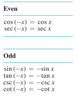
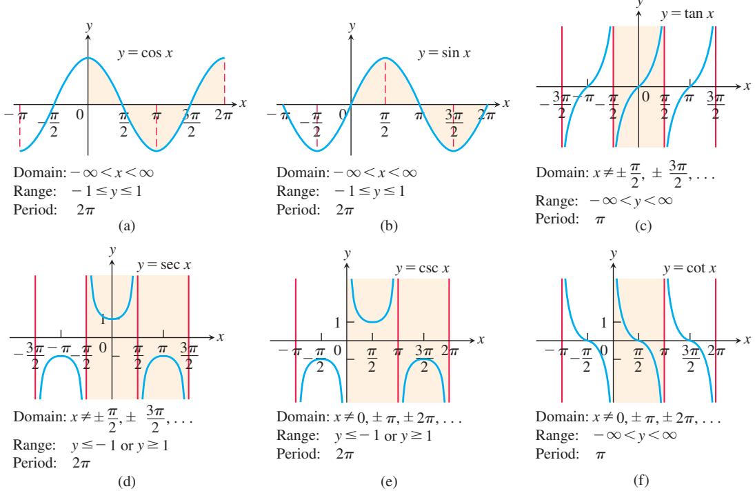
FIGURE 1.44 Graphs of the six basic trigonometric functions using radian measure. The shading for each trigonometric function indicates its periodicity.
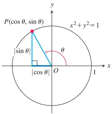
FIGURE 1.45 The reference triangle for a general angle
Trigonometric Identities
The coordinates of any point
When
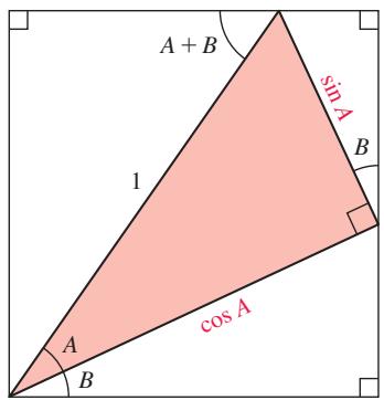
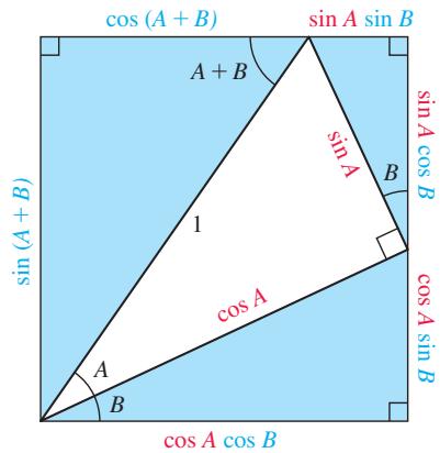
FIGURE 1.46 In a geometric proof of the angle sum identities we compare the opposite sides of the rectangle, which are equal. This assumes that A, B, and
This equation, true for all values of
The following formulas hold for all angles
Addition Formulas
There are similar formulas for
Double-Angle Formulas
Additional formulas come from combining the equations
We add the two equations to get
Half-Angle Formulas
The Law of Cosines
If a, b, and c are sides of a triangle ABC and if
This equation is called the law of cosines.
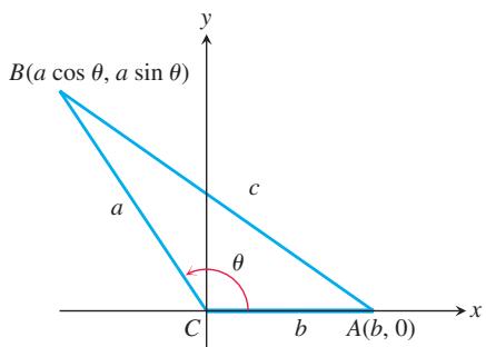
FIGURE 1.47 The square of the distance between A and B gives the law of cosines.
The law of cosines generalizes the Pythagorean theorem. If
To see why the law holds, we position the triangle in the xy-plane with the origin at C and the positive x-axis along one side of the triangle, as in Figure 1.47. The coordinates of A are
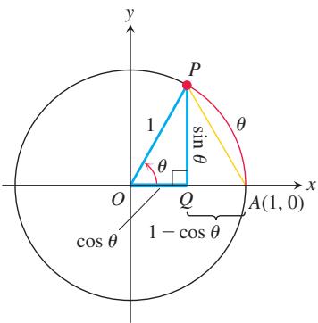
FIGURE 1.48 From the geometry of this figure, drawn for
Two Special Inequalities
For any angle
To establish these inequalities, we picture
Triangle APQ is a right triangle with sides of length
From the Pythagorean theorem and the fact that
The terms on the left-hand side of Equation (9) are both positive, so each is smaller than their sum and hence is less than or equal to
By taking square roots, this is equivalent to saying that
SO
These inequalities will be useful in the next chapter.
Transformations of Trigonometric Graphs
The rules for shifting, stretching, compressing, and reflecting the graph of a function summarized in the following diagram apply to the trigonometric functions we have discussed in this section.
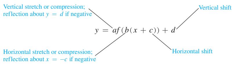
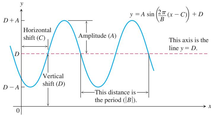
The transformation rules applied to the sine function give the general sine function or sinusoid formula
where
EXERCISES 1.3
Radians and Degrees
-
On a circle of radius 10 m, how long is an arc that subtends a central angle of (a)
4 𝜋 / 5 1 1 0 ∘ -
A central angle in a circle of radius 8 is subtended by an arc of length
1 0 𝜋 -
You want to make an
8 0 ∘
T 4. If you roll a 1-m-diameter wheel forward 30 cm over level ground, through what angle will the wheel turn? Answer in radians (to the nearest tenth) and degrees (to the nearest degree).
Evaluating Trigonometric Functions
- Copy and complete the following table of function values. If the function is undefined at a given angle, enter “UND.” Do not use a calculator or tables.
- Copy and complete the following table of function values. If the function is undefined at a given angle, enter “UND.” Do not use a calculator or tables.
In Exercises 7–12, one of
-
s i n 𝑥 = 3 5 , 𝑥 ∈ [ 𝜋 2 , 𝜋 ] -
t a n 𝑥 = 2 , 𝑥 ∈ [ 0 , 𝜋 2 ] -
c o s 𝑥 = 1 3 , 𝑥 ∈ [ − 𝜋 2 , 0 ] -
c o s 𝑥 = − 5 1 3 , 𝑥 ∈ [ 𝜋 2 , 𝜋 ] -
t a n 𝑥 = 1 2 , 𝑥 ∈ [ 𝜋 , 3 𝜋 2 ] -
s i n 𝑥 = − 1 2 , 𝑥 ∈ [ 𝜋 , 3 𝜋 2 ]
Graphing Trigonometric Functions
Graph the functions in Exercises 13–22. What is the period of each function?
-
s i n 2 𝑥 -
s i n ( 𝑥 / 2 ) -
c o s 𝜋 𝑥 -
c o s 𝜋 𝑥 2 -
− s i n 𝜋 𝑥 3 -
− c o s 2 𝜋 𝑥 -
c o s ( 𝑥 − 𝜋 2 ) -
s i n ( 𝑥 + 𝜋 6 ) -
s i n ( 𝑥 − 𝜋 4 ) + 1 -
c o s ( 𝑥 + 2 𝜋 3 ) − 2
Graph the functions in Exercises 23–26 in the ts-plane (t-axis horizontal, s-axis vertical). What is the period of each function? What symmetries do the graphs have?
-
𝑠 = c o t 2 𝑡 -
𝑠 = − t a n 𝜋 𝑡 -
𝑠 = s e c ( 𝜋 𝑡 2 ) -
𝑠 = c s c ( 𝑡 2 ) -
a. Graph
𝑦 = c o s 𝑥 𝑦 = s e c 𝑥 − 3 𝜋 / 2 ≤ 𝑥 ≤ 3 𝜋 / 2 𝑥 c o s 𝑥
b. Graph
-
Graph
𝑦 = t a n 𝑥 𝑦 = c o t 𝑥 − 7 ≤ 𝑥 ≤ 7 c o t 𝑥 t a n 𝑥 -
Graph
𝑦 = s i n 𝑥 𝑦 = ⌊ s i n 𝑥 ⌋ ⌊ s i n 𝑥 ⌋ -
Graph
𝑦 = s i n 𝑥 𝑦 = [ s i n 𝑥 ] [ s i n 𝑥 ]
Using the Addition Formulas
Use the addition formulas to derive the identities in Exercises 31–36.
-
c o s ( 𝑥 − 𝜋 2 ) = s i n 𝑥 -
c o s ( 𝑥 + 𝜋 2 ) = − s i n 𝑥 -
s i n ( 𝑥 + 𝜋 2 ) = c o s 𝑥 -
s i n ( 𝑥 − 𝜋 2 ) = − c o s 𝑥 -
c o s ( 𝐴 − 𝐵 ) = c o s 𝐴 c o s 𝐵 + s i n 𝐴 s i n 𝐵 -
s i n ( 𝐴 − 𝐵 ) = s i n 𝐴 c o s 𝐵 − c o s 𝐴 s i n 𝐵 -
What happens if you take B = A in the trigonometric identity
c o s ( 𝐴 − 𝐵 ) = c o s 𝐴 c o s 𝐵 + s i n 𝐴 s i n 𝐵 -
What happens if you take
𝐵 = 2 𝜋
In Exercises 39–42, express the given quantity in terms of
-
c o s ( 𝜋 + 𝑥 ) -
s i n ( 2 𝜋 − 𝑥 ) -
s i n ( 3 𝜋 2 − 𝑥 ) -
c o s ( 3 𝜋 2 + 𝑥 ) -
Evaluate
s i n 7 𝜋 1 2 s i n ( 𝜋 4 + 𝜋 3 ) -
Evaluate
c o s 1 1 𝜋 1 2 c o s ( 𝜋 4 + 2 𝜋 3 ) -
Evaluate
c o s 𝜋 1 2 -
Evaluate
s i n 5 𝜋 1 2
Using the Half-Angle Formulas
Find the function values in Exercises 47–50.
-
c o s 2 𝜋 8 -
c o s 2 5 𝜋 1 2 -
s i n 2 𝜋 1 2 -
s i n 2 3 𝜋 8
Solving Trigonometric Equations
For Exercises 51–54, solve for the angle
-
s i n 2 𝜃 = 3 4 -
s i n 2 𝜃 = c o s 2 𝜃 -
s i n 2 𝜃 − c o s 𝜃 = 0 -
c o s 2 𝜃 + c o s 𝜃 = 0
Theory and Examples
- The tangent sum formula of the sum of two angles is The standard formula for the tangent
Derive the formula.
-
(Continuation of Exercise 55.) Derive a formula for
t a n ( 𝐴 − 𝐵 ) -
Apply the law of cosines to the triangle in the accompanying figure to derive the formula for
c o s ( 𝐴 − 𝐵 )
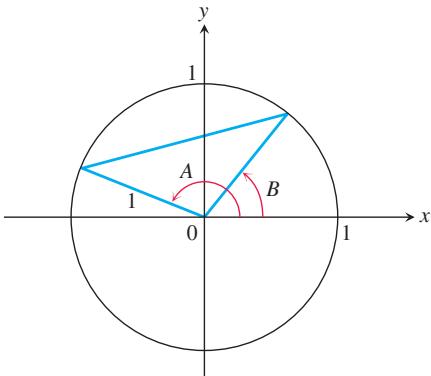
- a. Apply the formula for
c o s ( 𝐴 − 𝐵 ) s i n 𝜃 = c o s ( 𝜋 2 − 𝜃 ) s i n ( 𝐴 + 𝐵 )
b. Derive the formula for
-
A triangle has sides
𝑎 = 2 𝑏 = 3 𝐶 = 6 0 ∘ 𝑐 -
A triangle has sides
𝑎 = 2 𝑏 = 3 𝐶 = 4 0 ∘ 𝑐 -
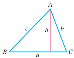
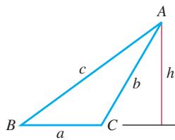
The law of sines The law of sines says that if
𝑎 , 𝑏 𝑐 𝐴 , 𝐵 𝐶
Use the accompanying figures and the identity
- A triangle has sides
𝑎 = 2 𝑏 = 3 𝐶 = 6 0 ∘ 𝐵

T 63. A triangle has side
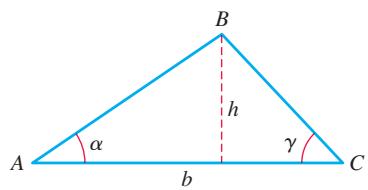
- Consider the length h of the perpendicular from point B to side b in the given triangle. Show that
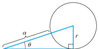
- Refer to the given figure. Write the radius
𝑟 𝛼 𝜃
- The approximation
s i n 𝑥 ≈ 𝑥 𝑥 s i n 𝑥 ≈ 𝑥 𝑥 | 𝑥 | < 0 . 1
a. With your grapher in radian mode, graph
b. With your grapher in degree mode, graph
General Sine Curves
For
identify A, B, C, and D for the sine functions in Exercises 67–70 and sketch their graphs.
-
𝑦 = 2 s i n ( 𝑥 + 𝜋 ) − 1 -
𝑦 = 1 2 s i n ( 𝜋 𝑥 − 𝜋 ) + 1 2 -
𝑦 = − 2 𝜋 s i n ( 𝜋 2 𝑡 ) + 1 𝜋 -
𝑦 = 𝐿 2 𝜋 s i n 2 𝜋 𝑡 𝐿 , 𝐿 > 0
COMPUTER EXPLORATIONS
In Exercises 71–74, you will explore graphically the general sine function
as you change the values of the constants A, B, C, and D. Use a CAS or computer grapher to perform the steps in the exercises.
- The period B Set the constants A = 3 and C = D = 0.
a. Plot
b. What happens to the graph for negative values of
- The horizontal shift C Set the constants A = 3, B = 6, D = 0.
a. Plot
b. What happens to the graph for negative values of
c. What smallest positive value should be assigned to
- The vertical shift D Set the constants A = 3, B = 6, C = 0.
a. Plot
b. What happens to the graph for negative values of
- The amplitude A Set the constants B = 6 and C = D = 0.
a. Describe what happens to the graph of the general sine function as A increases through positive values. Confirm your answer by plotting
b. What happens to the graph for negative values of
1.4 Exponential Functions
Exponential functions occur in a wide variety of applications, including interest rates, radioactive decay, population growth, the spread of a disease, consumption of natural resources, the earth’s atmospheric pressure, temperature change of a heated object placed in a cooler environment, and the dating of fossils. In this section we introduce these functions informally, using an intuitive approach. We give a rigorous development of them in Chapter 7, based on the ideas of integral calculus.
Exponential Behavior
When a positive quantity
Don’t confuse the exponential
such as
is the exponential function with base
EXAMPLE 1 In 2022, $100 is put into an investment account, where it grows by accruing interest that is compounded annually (once a year) at an interest rate of 5.5%. Assuming no additional funds are deposited to the account and no money is withdrawn, give a formula for a function describing the amount A in the account after x years have elapsed.
Solution If P = 100, at the end of the first year the amount in the account is the original amount plus the interest accrued, or
At the end of the second year the account earns interest again and grows to
Continuing this process, after x years the value of the account is
This is a multiple of the exponential function
TABLE 1.3 Investment account growth
| Year | Amount (dollars) | Yearly increase |
| 2022 | 100 | |
| 2023 | 5.50 | |
| 2024 | 5.80 | |
| 2025 | 6.12 | |
| 2026 | 6.46 |
In general, the amount after x years is given by
For integer and rational exponents, the value of an exponential function
If
If
which is the positive number that when multiplied by itself
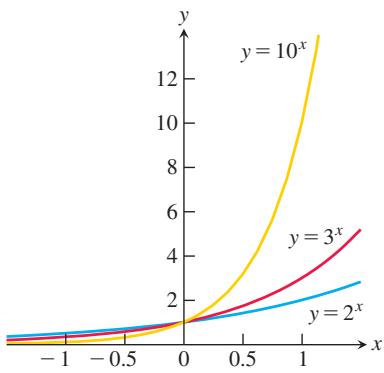
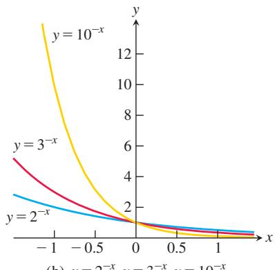
FIGURE 1.49 Graphs of exponential functions.
TABLE 1.4 Values of
| r | |
| 1.0 | 2.000000000 |
| 1.7 | 3.249009585 |
| 1.73 | 3.317278183 |
| 1.732 | 3.321880096 |
| 1.7320 | 3.321880096 |
| 1.73205 | 3.321995226 |
| 1.732050 | 3.321995226 |
| 1.7320508 | 3.321997068 |
| 1.73205080 | 3.321997068 |
| 1.732050808 | 3.321997086 |
When
The graphs of several exponential functions are shown in Figure 1.49. These graphs show the values of the exponential functions for real inputs x. We choose the value of
We illustrate how to define the value of an exponential function at an irrational power using the exponential function
We then consider the list of powers of 2 with more and more digits in the decimal expansion,
We know the meaning of each number in list (1) because the successive decimal approximations to
Table 1.4 illustrates how taking better approximations to
Exponential functions obey the rules of exponents listed below. It is easy to check these rules using algebra when the exponents are integers or rational numbers. We prove them for all real exponents in Chapter 7.
Rules for Exponents
If
EXAMPLE 2 We use the rules for exponents to simplify some numerical expressions.
3 1 . 1 ⋅ 3 0 . 7 = 3 1 . 1 + 0 . 7 = 3 1 . 8
-
( 5 √ 2 ) √ 2 = 5 √ 2 ⋅ √ 2 = 5 2 = 2 5 -
7 𝜋 ⋅ 8 𝜋 = ( 5 6 ) 𝜋
The Natural Exponential Function 𝑒 𝑥
The most important exponential function used for modeling natural, physical, and economic phenomena is the natural exponential function, whose base is the special number e. The number e is irrational, and its value to nine decimal places is 2.718281828. (In Section 3.8 we will see a way to calculate the value of e.) It might seem strange that we would use this number for a base rather than a simple number like 2 or 10. The advantage in using e as a base is that it greatly simplifies many of the calculations in calculus.
In Figure 1.49a you can see that for
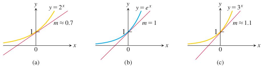
FIGURE 1.50 Among the exponential functions, the graph of
Exponential Growth and Decay
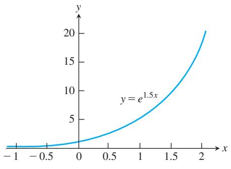
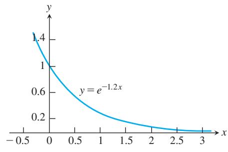
The function
(a)
(b)
FIGURE 1.51 Graphs of (a) exponential growth, k = 1.5 > 0, and (b) exponential decay, k = -1.2 < 0.
EXAMPLE 3 Investment companies often use the model
Solution Let t = 0 represent 2022, t = 1 represent 2023, and so on. Then the exponential growth model is
This compares with $123.88 in the account when the interest is compounded annually, as was done in Example 1.
EXAMPLE 4 Laboratory experiments indicate that some atoms emit a part of their mass as radiation, with the remainder of the atom re-forming to make an atom of some new element. For example, radioactive carbon-14 decays into nitrogen; radium eventually decays into lead. If
The number r is called the decay rate of the radioactive substance. (We will see how this formula is obtained in Section 7.2.) For carbon-14, the decay rate has been determined experimentally to be about
Solution If we start with an amount
That is, after 866 years, we are left with about
You may wonder why we use the family of functions
EXERCISES 1.4
Sketching Exponential Curves
In Exercises 1–6, sketch the given curves together in the appropriate coordinate plane, and label each curve with its equation.
-
𝑦 = 2 𝑥 , 𝑦 = 4 𝑥 , 𝑦 = 3 − 𝑥 , 𝑦 = ( 1 / 5 ) 𝑥 -
𝑦 = 3 𝑥 , 𝑦 = 8 𝑥 , 𝑦 = 2 − 𝑥 , 𝑦 = ( 1 / 4 ) 𝑥 -
𝑦 = 2 − 𝑡 𝑦 = − 2 𝑡 -
𝑦 = 3 − 𝑡 𝑦 = − 3 𝑡 -
𝑦 = 𝑒 𝑥 𝑦 = 1 / 𝑒 𝑥 -
𝑦 = − 𝑒 𝑥 a n d 𝑦 = − 𝑒 − 𝑥
In each of Exercises 7–10, sketch the shifted exponential curves.
-
𝑦 = 2 𝑥 − 1 𝑦 = 2 − 𝑥 − 1 -
𝑦 = 3 𝑥 + 2 𝑦 = 3 − 𝑥 + 2 -
𝑦 = 1 − 𝑒 𝑥 𝑦 = 1 − 𝑒 − 𝑥 -
𝑦 = − 1 − 𝑒 𝑥 𝑦 = − 1 − 𝑒 − 𝑥
Applying the Laws of Exponents
Use the laws of exponents to simplify the expressions in Exercises 11–20.
-
1 6 2 ⋅ 1 6 − 1 . 7 5 -
9 1 / 3 ⋅ 9 1 / 6 -
4 4 . 2 4 3 . 7 -
3 5 / 3 3 2 / 3 -
( 2 5 1 / 8 ) 4 -
( 1 3 √ 2 ) √ 2 / 2 -
2 √ 3 ⋅ 7 √ 3 -
( √ 3 ) 1 / 2 ⋅ ( √ 1 2 ) 1 / 2 -
( 2 √ 2 ) 4 -
( √ 6 3 ) 2
Compositions Involving Exponential Functions
Find the domain and range for each of the functions in Exercises 21–24.
-
𝑓 ( 𝑥 ) = 1 2 + 𝑒 𝑥 -
𝑔 ( 𝑡 ) = c o s ( 𝑒 − 𝑡 ) -
𝑔 ( 𝑡 ) = √ 1 + 3 − 𝑡 -
𝑓 ( 𝑥 ) = 3 1 − 𝑒 2 𝑥
Applications
T In Exercises 25–28, use graphs to find approximate solutions.
-
2 𝑥 = 5 -
𝑒 𝑥 = 4 -
3 𝑥 − 0 . 5 = 0 -
3 − 2 − 𝑥 = 0
In Exercises 29–36, use an exponential model and a graphing calculator to estimate the answer in each problem.
-
Population growth The population of a midwestern city is 500,000 and is increasing at the rate of
3 . 7 5 % -
Population growth The population of Silver Run in the year 1890 was 6250. Assume the population increased at a rate of 2.75% per year.
a. Estimate the population in 1915 and 1940.
b. Approximately when did the population reach 50,000?
- Radioactive decay The half-life of phosphorus-32 is about 14 days. There are 6.6 grams present initially.
a. Express the amount of phosphorus-32 remaining as a function of time t.
b. When will there be 1 gram remaining?
-
If Jean invests
2 3 0 0 𝑖 𝑛 𝑎 𝑟 𝑒 𝑡 𝑖 𝑟 𝑒 𝑚 𝑒 𝑛 𝑡 𝑎 𝑐 𝑐 𝑜 𝑢 𝑛 𝑡 𝑤 𝑖 𝑡 ℎ 𝑎 6 -
Doubling your money Determine how much time is required for an investment to double in value if interest is earned at the rate of 6.25% compounded annually.
-
Tripling your money Determine how much time is required for an investment to triple in value if interest is earned at the rate of 5.75% compounded continuously.
-
Cholera bacteria Suppose that a colony of bacteria starts with 1 bacterium and doubles in number every half hour. How many bacteria will the colony contain at the end of 24 hours?
-
Eliminating a disease Suppose that in any given year the number of cases of a disease is reduced by
2 0 %
a. to reduce the number of cases to 1000?
b. to eliminate the disease; that is, to reduce the number of cases to less than 1?
1.5 Inverse Functions and Logarithms
A function that undoes, or inverts, the effect of a function f is called the inverse of f. Many common functions, though not all, are paired with an inverse. In this section we present the natural logarithmic function
One-to-One Functions
A function is a rule that assigns a value from its range to each element in its domain. Some functions assign the same range value to more than one element in the domain. The function
DEFINITION A function
is one-to-one on a domain 𝑓 ( 𝑥 ) if 𝐷 whenever 𝑓 ( 𝑥 1 ) ≠ 𝑓 ( 𝑥 2 ) in 𝑥 1 ≠ 𝑥 2 . 𝐷
EXAMPLE 1 Some functions are one-to-one on their entire natural domain. Other functions are not one-to-one on their entire domain, but by restricting the function to a smaller domain we can create a function that is one-to-one. The original and restricted functions are not the same functions, because they have different domains. However, the two functions have the same values on the smaller domain.
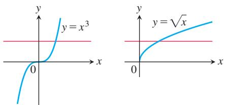
(a) One-to-one: Graph meets each horizontal line at most once.
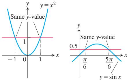
(b) Not one-to-one: Graph meets one or more horizontal lines more than once.
FIGURE 1.52 (a)
Caution
Do not confuse the inverse function
(a)
(b)
The graph of a one-to-one function
The Horizontal Line Test for One-to-One Functions
A function
Inverse Functions
Since each output of a one-to-one function comes from just one input, the effect of the function can be inverted to send each output back to the input from which it came.
DEFINITION Suppose that
is a one-to-one function on a domain 𝑓 with range 𝐷 . The inverse function 𝑅 is defined by 𝑓 − 1 𝑓 − 1 ( 𝑏 ) = 𝑎 i f 𝑓 ( 𝑎 ) = 𝑏 .
The domain of
The symbol
EXAMPLE 2 Suppose a one-to-one function
| x | 1 | 2 | 3 | 4 | 5 | 6 | 7 | 8 |
| f(x) | 3 | 4.5 | 7 | 10.5 | 15 | 20.5 | 27 | 34.5 |
A table for the values of
| y | 3 | 4.5 | 7 | 10.5 | 15 | 20.5 | 27 | 34.5 |
| 1 | 2 | 3 | 4 | 5 | 6 | 7 | 8 |
If we apply f to send an input x to the output
Only a one-to-one function can have an inverse. The reason is that if
Suppose f is a function whose domain is an interval. If f is increasing, then it satisfies the inequality
Finding Inverses
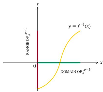
The graphs of a function and its inverse are closely related. To read the value of a function from its graph, we start at a point x on the x-axis, go vertically to the graph, and then move horizontally to the y-axis to read the value of y. The inverse function can be read from the graph by reversing this process. Start with a point y on the y-axis, go horizontally to the graph of
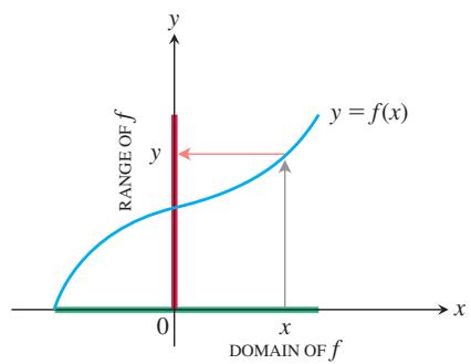
(a) To find the value of f at x, we start at x, go up to the curve, and then move to the y-axis.
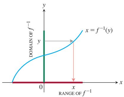
(b) The graph of
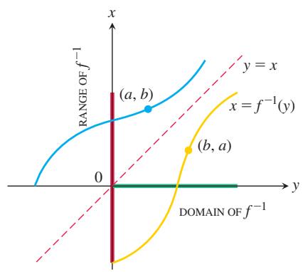
(c) To draw the graph of
(d) Then we interchange the letters
FIGURE 1.53 The graph of
We want to set up the graph of
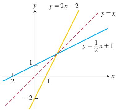
FIGURE 1.54 Graphing
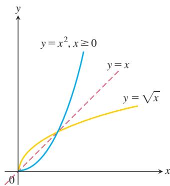
FIGURE 1.55 The functions
The process of passing from f to
-
Solve the equation
𝑦 = 𝑓 ( 𝑥 ) 𝑥 𝑥 = 𝑓 − 1 ( 𝑦 ) 𝑥 𝑦 -
Interchange
𝑥 𝑦 𝑦 = 𝑓 − 1 ( 𝑥 ) 𝑓 − 1 𝑥 𝑦
EXAMPLE 3 Find the inverse of
The graph satisfies the horizontal line test, so the function is one-to-one (Fig. 1.59).
- Interchange x and y: y = 2x - 2.
Expresses the function in the usual form, where y is the dependent variable.
The inverse of the function
EXAMPLE 4 Find the inverse of the function
Solution For
We then interchange x and y, obtaining
The inverse of the function
Notice that the function
Logarithmic Functions
If
DEFINITION The logarithm function with base a, written
, is the inverse of the base a exponential function 𝑦 = l o g 𝑎 𝑥 . 𝑦 = 𝑎 𝑥 ( 𝑎 > 0 , 𝑎 ≠ 1 )
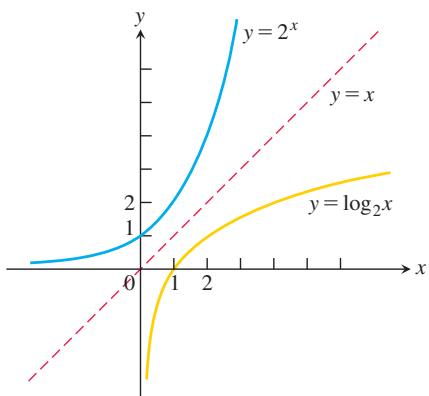
(a)
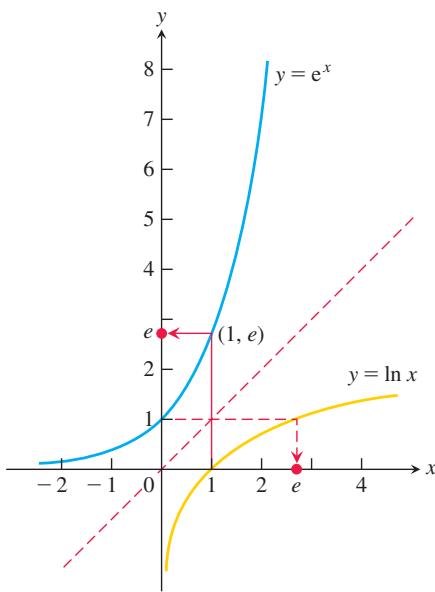
(b)
FIGURE 1.56 (a) The graphs of
HISTORICAL BIOGRAPHY
John Napier (1550–1617)
Scotsman John Napier went to St. Salvator’s College in St. Andrews, where he studied from mathematician John Rutherford. Today, Napier is best known as the inventor of logarithms.
To know more, visit the companion Website.
The domain of
Figure 1.56a shows the graph of
Because we have no technique yet for solving the equation
Logarithms with base 2 are often used when working with binary numbers, as is common in computer science. Logarithms with base e and base 10 are so important in applications that many calculators have special keys for them. They also have their own special notation and names:
The function
In particular, because
Properties of Logarithms
Logarithms, invented by John Napier, were the single most important improvement in arithmetic calculation before the modern electronic computer. The properties of logarithms reduce multiplication of positive numbers to addition of their logarithms, division of positive numbers to subtraction of their logarithms, and exponentiation of a number to multiplying its logarithm by the exponent.
We summarize these properties for the natural logarithm as a series of rules that we prove in Chapter 7.
THEOREM 1—Algebraic Properties of the Natural Logarithm
For any numbers
- Product Rule:
- Quotient Rule:
- Reciprocal Rule:
Rule 2 with
- Power Rule:
Inverse Properties for
EXAMPLE 5 We use the properties in Theorem 1 to rewrite three expressions.
(a)
(b)
(c)
Because
Substituting
Thus, the exponential function
Every exponential function is a power of the natural exponential function.
That is,
For example,
Returning once more to the properties of
Rewriting this equation as
Change-of-Base Formula
Every logarithmic function is a constant multiple of the natural logarithm.
Applications
In Section 1.4 we looked at examples of exponential growth and decay problems. Here we use properties of logarithms to answer more questions concerning such problems.
EXAMPLE 6 If
Solution From Example 1, Section 1.4, with P = 1000 and r = 0.0525, the amount in the account at any time t in years is
Thus we have
The amount in the account will reach $2500 in 18 years, when the annual interest payment is deposited for that year.
EXAMPLE 7 The half-life of a radioactive element is the time expected to pass until half of the radioactive nuclei present in a sample decay. The half-life is a constant that does not depend on the number of radioactive nuclei initially present in the sample, but only on the radioactive substance.
To compute the half-life, let
This value of
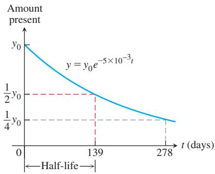
FIGURE 1.57 Amount of polonium-210 present at time t, where
The effective radioactive lifetime of polonium-210 is so short that we measure it in days rather than years. The number of radioactive atoms remaining after t days in a sample that starts with
The element’s half-life is
This means that after 139 days,
Inverse Trigonometric Functions
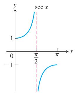
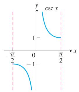
The six basic trigonometric functions are not one-to-one (since their values repeat periodically). However, we can restrict their domains to intervals on which they are one-to-one. The sine function increases from -1 at
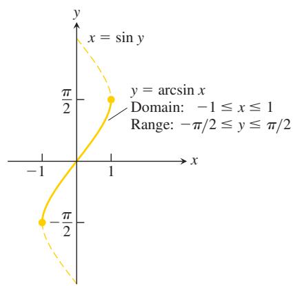
FIGURE 1.58 The graph of
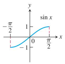
Domain:
(b)
Domain restrictions that make the trigonometric functions one-to-one
(a)
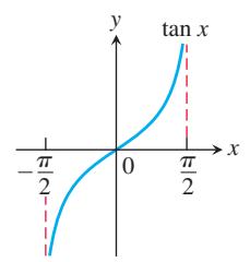
FIGURE 1.59 The graphs of
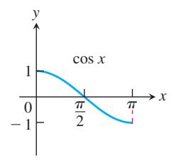
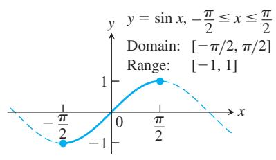
domain to the interval
(a)
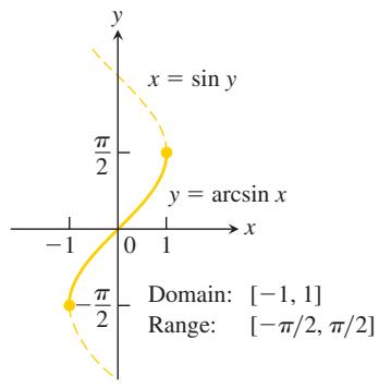
Range:
Range:
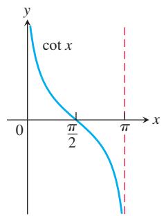
Domain:
Range:
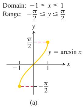
Domain:
Range:
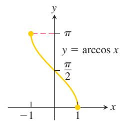
Domain:
Range:
Since these restricted functions are now one-to-one, they have inverses, which we denote by
These equations are read “y equals the arcsine of x” or “y equals arcsin x” and so on.
Caution The -1 in the expressions for the inverse means “inverse.” It does not mean reciprocal. For example, the reciprocal of
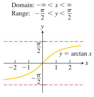
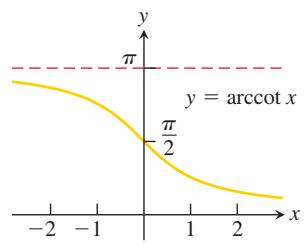
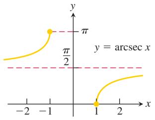
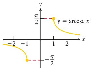
The graphs of the six inverse trigonometric functions are obtained by reflecting the graphs of the restricted trigonometric functions through the line y = x. Figure 1.59b shows the graph of
The Arcsine and Arcosine Functions
We define the arcsine and arccosine as functions whose values are angles (measured in radians) that belong to restricted domains of the sine and cosine functions.
(b)
(c)
Domain:
Domain:
(d)
(e)
(f)
FIGURE 1.60 Graphs of the six basic inverse trigonometric functions.
The “Arc” in Arcsine and Arccosine
For a unit circle and radian angles, the arc length equation
The graph of
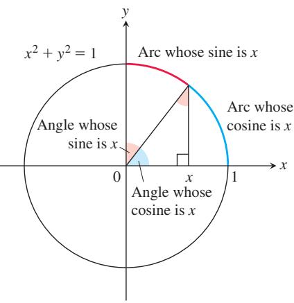
The graph of
EXAMPLE 8 Evaluate (a) arcsin
Solution
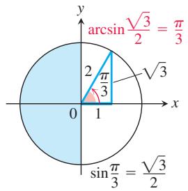
(a) We see that
because
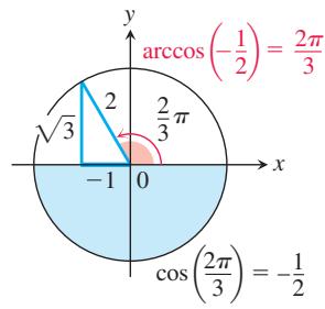
(b) We have
because
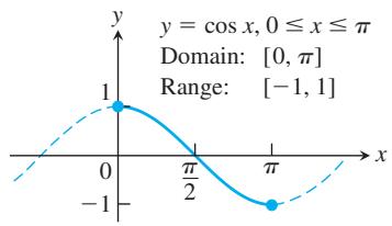
(a)
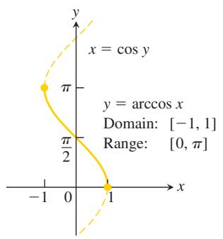
(b)
FIGURE 1.61 The graphs of (a)
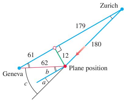
FIGURE 1.63 Diagram for drift correction (Example 9), with distances rounded to the nearest kilometer (drawing not to scale).
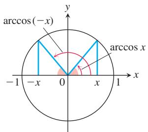
FIGURE 1.64 arccos x and arccos
Using the same procedure illustrated in Example 8, we can create the following table of common values for the arcsine and arccosine functions.
| x | arcsin x | arccos x |
(a)
(b)
FIGURE 1.62 Values of the arcsine and arccosine functions (Example 8).
EXAMPLE 9 During a 240-km airplane flight from Zurich to Geneva, after flying 180 km the navigator determines that the plane is 12 km off course, as shown in Figure 1.63. Find the angle a for a course parallel to the original correct course, the angle b, and the drift correction angle
Solution From the Pythagorean theorem and given information, we compute an approximate hypothetical flight distance of 179 km, had the plane been flying along the original correct course (see Figure 1.63). Knowing the flight distance from Zurich to Geneva, we next calculate the remaining leg of the original course to be 61 km. Applying the Pythagorean theorem again then gives an approximate distance of 62 km from the position of the plane to Geneva. Finally, from Figure 1.63, we see that
Identities Involving Arcsine and Arccosine
As we can see from Figure 1.64, the arccosine of x satisfies the identity
or
Also, we can see from the triangle in Figure 1.65 that for x > 0,
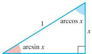
FIGURE 1.65 arcsin x and arccos x are complementary angles (so their sum is
Equation (5) holds for the other values of x in
The arctangent, arccotangent, arcsecant, and arccosecant functions are defined in Section 3.9. There we develop additional properties of the inverse trigonometric functions using the identities discussed here.
EXERCISES 1.5
Identifying One-to-One Functions Graphically
Which of the functions graphed in Exercises 1–6 are one-to-one, and which are not?
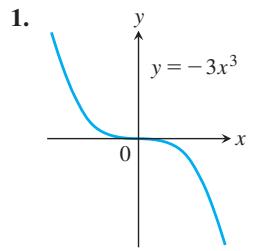
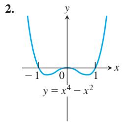
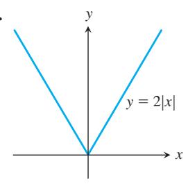
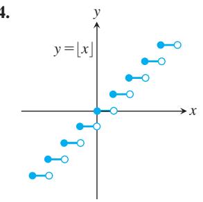
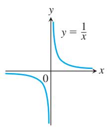
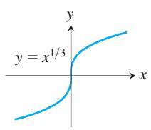
In Exercises 7–10, determine from its graph whether the function is one-to-one.
-
𝑓 ( 𝑥 ) = { 3 − 𝑥 , 𝑥 < 0 3 , 𝑥 ≥ 0 -
𝑓 ( 𝑥 ) = { 2 𝑥 + 6 , 𝑥 ≤ − 3 𝑥 + 4 , 𝑥 > − 3 -
𝑓 ( 𝑥 ) = { 1 − 𝑥 2 , 𝑥 ≤ 0 𝑥 𝑥 + 2 , 𝑥 > 0 -
𝑓 ( 𝑥 ) = { 2 − 𝑥 2 , 𝑥 ≤ 1 𝑥 2 , 𝑥 > 1
Graphing Inverse Functions
Each of Exercises 11–16 shows the graph of a function
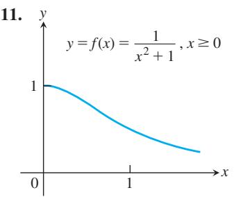
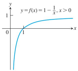
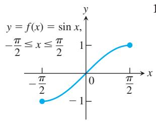
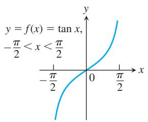
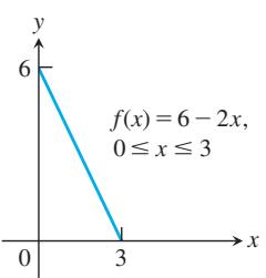
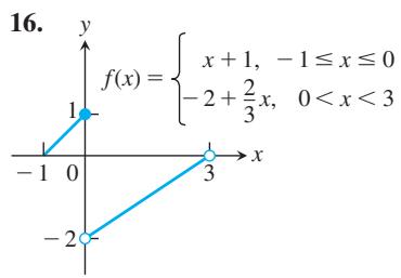
- a. Graph the function
𝑓 ( 𝑥 ) = √ 1 − 𝑥 2 , 0 ≤ 𝑥 ≤ 1
b. Show that
- a. Graph the function
𝑓 ( 𝑥 ) = 1 / 𝑥
b. Show that
Formulas for Inverse Functions
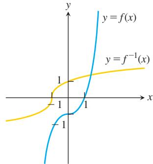
Each of Exercises 19–24 gives a formula for a function
𝑓 ( 𝑥 ) = 𝑥 2 + 1 , 𝑥 ≥ 0
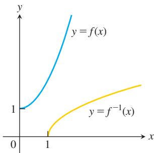
𝑓 ( 𝑥 ) = 𝑥 2 , 𝑥 ≤ 0
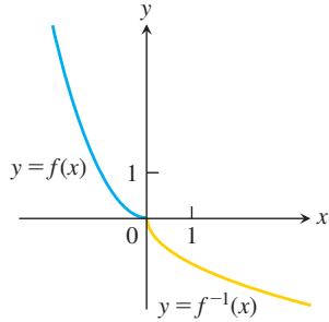
-
𝑓 ( 𝑥 ) = 𝑥 3 − 1 -
𝑓 ( 𝑥 ) = 𝑥 2 − 2 𝑥 + 1 , 𝑥 ≥ 1
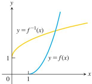
-
𝑓 ( 𝑥 ) = ( 𝑥 + 1 ) 2 𝑥 ≥ − 1 -
𝑓 ( 𝑥 ) = 𝑥 2 / 3 𝑥 ≥ 0
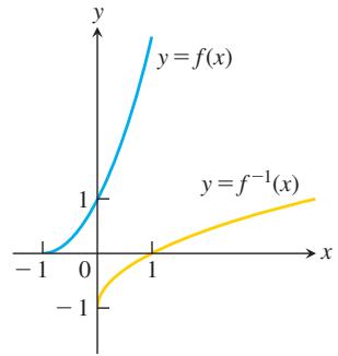
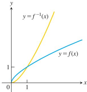
Each of Exercises 25–36 gives a formula for a function
-
𝑓 ( 𝑥 ) = 𝑥 5 -
𝑓 ( 𝑥 ) = 𝑥 4 , 𝑥 ≥ 0 -
𝑓 ( 𝑥 ) = 𝑥 3 + 1 -
𝑓 ( 𝑥 ) = ( 1 / 2 ) 𝑥 − 7 / 2 -
𝑓 ( 𝑥 ) = 1 / 𝑥 2 , 𝑥 > 0 -
𝑓 ( 𝑥 ) = 1 / 𝑥 3 , 𝑥 ≠ 0 -
𝑓 ( 𝑥 ) = 𝑥 + 3 𝑥 − 2 -
𝑓 ( 𝑥 ) = √ 𝑥 √ 𝑥 − 3 -
𝑓 ( 𝑥 ) = 𝑥 2 − 2 𝑥 , 𝑥 ≤ 1 -
𝑓 ( 𝑥 ) = ( 2 𝑥 3 + 1 ) 1 / 5
(Hint: Complete the square.)
-
𝑓 ( 𝑥 ) = 𝑥 + 𝑏 𝑥 − 2 , 𝑏 > − 2 -
𝑓 ( 𝑥 ) = 𝑥 2 − 2 𝑏 𝑥 , 𝑏 > 0 𝑥 ≤ 𝑏
Inverses of Lines
- a. Find the inverse of the function
𝑓 ( 𝑥 ) = 𝑚 𝑥
b. What can you conclude about the inverse of a function
-
Show that the graph of the inverse of
𝑓 ( 𝑥 ) = 𝑚 𝑥 + 𝑏 𝑚 𝑏 𝑚 ≠ 0 1 / 𝑚 𝑦 − 𝑏 / 𝑚 -
a. Find the inverse of
𝑓 ( 𝑥 ) = 𝑥 + 1
b. Find the inverse of
c. What can you conclude about the inverses of functions whose graphs are lines parallel to the line
- a. Find the inverse of
𝑓 ( 𝑥 ) = − 𝑥 + 1 𝑦 = − 𝑥 + 1 𝑦 = 𝑥
b. Find the inverse of
c. What can you conclude about the inverses of functions whose graphs are lines perpendicular to the line
Logarithms and Exponentials
-
Express the following logarithms in terms of
l n 2 l n 3
a.l n 0 . 7 5 l n ( 4 / 9 ) l n ( 1 / 2 ) l n 3 √ 9 l n 3 √ 2 l n √ 1 3 . 5 -
Express the following logarithms in terms of
l n 5 l n 7
a.l n ( 1 / 1 2 5 ) l n 9 . 8 l n 7 √ 7 l n 1 2 2 5 l n 0 . 0 5 6 ( l n 3 5 + l n ( 1 / 7 ) ) / ( l n 2 5 )
Use the properties of logarithms to write the expressions in Exercises 43 and 44 as a single term.
-
a.
l n s i n 𝜃 − l n ( s i n 𝜃 5 ) l n ( 3 𝑥 2 − 9 𝑥 ) + l n ( 1 3 𝑥 ) 1 2 l n ( 4 𝑡 4 ) − l n 𝑏 -
a.
l n s e c 𝜃 + l n c o s 𝜃 l n ( 8 𝑥 + 4 ) − 2 l n 𝑐 3 l n 3 √ 𝑡 2 − 1 − l n ( 𝑡 + 1 )
Find simpler expressions for the quantities in Exercises 45–48.
-
a.
𝑒 l n 7 . 2 𝑒 − l n 𝑥 2 𝑒 l n 𝑥 − l n 𝑦 -
a.
𝑒 l n ( 𝑥 2 + 𝑦 2 ) 𝑒 − l n 0 . 3 𝑒 l n 𝜋 𝑥 − l n 2 -
a.
2 l n √ 𝑒 l n ( l n 𝑒 𝑒 ) l n ( 𝑒 − 𝑥 2 − 𝑦 2 ) -
a.
l n ( 𝑒 s e c 𝜃 ) l n ( 𝑒 ( 𝑒 𝑥 ) ) l n ( 𝑒 2 l n 𝑥 )
In Exercises 49–54, solve for y in terms of t or x, as appropriate.
-
l n 𝑦 = 2 𝑡 + 4 -
l n 𝑦 = − 𝑡 + 5 -
l n ( 𝑦 − 𝑏 ) = 5 𝑡 -
l n ( 𝑐 − 2 𝑦 ) = 𝑡 -
l n ( 𝑦 − 1 ) − l n 2 = 𝑥 + l n 𝑥 -
l n ( 𝑦 2 − 1 ) − l n ( 𝑦 + 1 ) = l n ( s i n 𝑥 )
In Exercises 55 and 56, solve for
55. a.
- a.
𝑒 5 𝑘 = 1 4 8 0 𝑒 𝑘 = 1 𝑒 ( l n 0 . 8 ) 𝑘 = 0 . 8
In Exercises 57–64, solve for t.
-
a.
𝑒 − 0 . 3 𝑡 = 2 7 𝑒 𝑘 𝑡 = 1 2 𝑒 ( l n 0 . 2 ) 𝑡 = 0 . 4 -
a.
𝑒 − 0 . 0 1 𝑡 = 1 0 0 0 𝑒 𝑘 𝑡 = 1 1 0 𝑒 ( l n 2 ) 𝑡 = 1 2 -
𝑒 √ 𝑡 = 𝑥 2 -
𝑒 ( 𝑥 2 ) 𝑒 ( 2 𝑥 + 1 ) = 𝑒 𝑡 -
𝑒 2 𝑡 − 3 𝑒 𝑡 = 0 -
𝑒 − 2 𝑡 + 6 = 5 𝑒 − 𝑡 -
l n ( 𝑡 𝑡 − 1 ) = 2 -
l n ( 𝑡 − 2 ) = l n 8 − l n 𝑡 -
a.
5 l o g 5 7 8 l o g 8 √ 2 1 . 3 l o g 1 . 3 7 5 l o g 4 1 6 l o g 3 √ 3 l o g 4 ( 1 4 ) -
a.
2 l o g 2 3 l o g 1 1 1 2 1 1 0 l o g 1 0 ( 1 / 2 ) l o g 1 2 1 1 1 𝜋 l o g 𝜋 7 l o g 3 ( 1 9 ) -
a.
2 l o g 4 𝑥 9 l o g 3 𝑥 l o g 2 ( 𝑒 ( l n 2 ) ( s i n 𝑥 ) ) -
a.
2 5 l o g 5 ( 3 𝑥 2 ) l o g 𝑒 ( 𝑒 𝑥 ) l o g 4 ( 2 𝑒 𝑥 s i n 𝑥 )
Express the ratios in Exercises 69 and 70 as ratios of natural logarithms and simplify.
69. a.
- a.
l o g 9 𝑥 l o g 3 𝑥 l o g √ 1 0 𝑥 l o g √ 2 𝑥 l o g 𝑎 𝑏 l o g 𝑏 𝑎
Arcsine and Arcosine
In Exercises 71–74, find the exact value of each expression. Remember that
-
a.
c o s − 1 ( 1 2 ) c o s − 1 ( − 1 √ 2 ) c o s − 1 ( √ 3 2 ) -
a. arccos
( − 1 ) -
a.
a r c s i n ( − 1 ) a r c s i n ( − 1 √ 2 )
Theory and Examples
-
If
𝑓 ( 𝑥 ) 𝑔 ( 𝑥 ) = − 𝑓 ( 𝑥 ) -
If
𝑓 ( 𝑥 ) 𝑓 ( 𝑥 ) ℎ ( 𝑥 ) = 1 / 𝑓 ( 𝑥 ) -
Suppose that the range of g lies in the domain of f so that the composition
𝑓 ∘ 𝑔 𝑓 ∘ 𝑔 -
If a composition
𝑓 ∘ 𝑔 𝑔 -
Find a formula for the inverse function
𝑓 − 1 ( 𝑓 ∘ 𝑓 − 1 ) ( 𝑥 ) = ( 𝑓 − 1 ∘ 𝑓 ) ( 𝑥 ) = 𝑥
a.𝑓 ( 𝑥 ) = 1 0 0 1 + 2 − 𝑥 𝑓 ( 𝑥 ) = 5 0 1 + 1 . 1 − 𝑥 𝑓 ( 𝑥 ) = 𝑒 𝑥 − 1 𝑒 𝑥 + 1 𝑓 ( 𝑥 ) = l n 𝑥 2 − l n 𝑥 -
The identity arcsin
𝑥 + a r c c o s 𝑥 = 𝜋 / 2 -
Start with the graph of
𝑦 = l n 𝑥
a. shifting down 3 units.
b. shifting right 1 unit.
c. shifting left 1, up 3 units.
d. shifting down 4, right 2 units.
e. reflecting about the𝑦
f. reflecting about the line𝑦 = 𝑥 -
Start with the graph of
𝑦 = l n 𝑥 -
The equation
𝑥 2 = 2 𝑥 𝑥 = 2 , 𝑥 = 4 -
Could
𝑥 l n 2 2 l n 𝑥 -
Radioactive decay The half-life of a certain radioactive substance is 12 hours. There are 8 grams present initially.
a. Express the amount of substance remaining as a function of time t.
b. When will there be 1 gram remaining?
-
Doubling your money Determine how much time is required for a $500 investment to double in value if interest is earned at the rate of 4.75% compounded annually.
-
Population growth The population of a town in California is 375,000 and is increasing at the rate of 2.25% per year. Predict when the population will be 1 million.
-
Radon-222 The decay equation for radon-222 gas is known to be
𝑦 = 𝑦 0 𝑒 − 0 . 1 8 𝑡
CHAPTER 1 Questions to Guide Your Review
-
What is a function? What is its domain? Its range? What is an arrow diagram for a function? Give examples.
-
What is the graph of a real-valued function of a real variable? What is the vertical line test?
-
What is a piecewise-defined function? Give examples.
-
What are the important types of functions frequently encountered in calculus? Give an example of each type.
-
What is meant by an increasing function? A decreasing function? Give an example of each.
-
What is an even function? An odd function? What symmetry properties do the graphs of such functions have? What advantage can we take of this? Give an example of a function that is neither even nor odd.
-
If
𝑓 𝑔 𝑓 + 𝑔 , 𝑓 − 𝑔 , 𝑓 𝑔 𝑓 / 𝑔 𝑓 𝑔 -
When is it possible to compose one function with another? Give examples of compositions and their values at various points. Does the order in which functions are composed ever matter?
-
How do you change the equation
𝑦 = 𝑓 ( 𝑥 ) | 𝑘 | -
How do you change the equation
𝑦 = 𝑓 ( 𝑥 ) -
What is radian measure? How do you convert from radians to degrees? Degrees to radians?
-
Graph the six basic trigonometric functions. What symmetries do the graphs have?
-
What is a periodic function? Give examples. What are the periods of the six basic trigonometric functions?
-
Starting with the identity
s i n 2 𝜃 + c o s 2 𝜃 = 1 c o s ( 𝐴 + 𝐵 ) s i n ( 𝐴 + 𝐵 ) -
How does the formula for the general sine function
𝑓 ( 𝑥 ) = 𝐴 s i n ( ( 2 𝜋 / 𝐵 ) ( 𝑥 − 𝐶 ) ) + 𝐷 -
Name three issues that arise when functions are graphed using a calculator or computer with graphing software. Give examples.
-
What is an exponential function? Give examples. What laws of exponents does it obey? How does it differ from a simple power function like
𝑓 ( 𝑥 ) = 𝑥 𝑛 -
What is the number
𝑒 𝑓 ( 𝑥 ) = 𝑒 𝑥 𝑒 𝑥 𝑥 2 , 𝑥 3 -
What functions have inverses? How do you know if two functions f and g are inverses of one another? Give examples of functions that are (are not) inverses of one another.
-
How are the domains, ranges, and graphs of functions and their inverses related? Give an example.
-
What procedure can you sometimes use to express the inverse of a function of
𝑥 𝑥 -
What is a logarithmic function? What properties does it satisfy? What is the natural logarithm function? What are the domain and range of
𝑦 = l n 𝑥 -
How is the graph of
l o g 𝑎 𝑥 l n 𝑥 -
How are the inverse trigonometric functions defined? How can you sometimes use right triangles to find values of these functions? Give examples.
CHAPTER 1 Practice Exercises
Functions and Graphs
-
Express the area and circumference of a circle as functions of the circle’s radius. Then express the area as a function of the circumference.
-
Express the radius of a sphere as a function of the sphere’s surface area. Then express the surface area as a function of the volume.
-
A point P in the first quadrant lies on the parabola
𝑦 = 𝑥 2 -
A hot-air balloon rising straight up from a level field is tracked by a range finder located 500 m from the point of liftoff. Express the balloon’s height as a function of the angle the line from the range finder to the balloon makes with the ground.
In Exercises 5–8, determine whether the graph of the function is symmetric about the y-axis, the origin, or neither.
-
𝑦 = 𝑥 1 / 5 -
𝑦 = 𝑥 2 / 5 -
𝑦 = 𝑥 2 − 2 𝑥 − 1 -
𝑦 = 𝑒 − 𝑥 2
In Exercises 9–16, determine whether the function is even, odd, or neither.
-
𝑦 = 𝑥 5 − 𝑥 3 − 𝑥 -
𝑦 = 1 − c o s 𝑥 -
𝑦 = s e c 𝑥 t a n 𝑥 -
𝑦 = 𝑥 4 + 1 𝑥 3 − 2 𝑥 -
𝑦 = 𝑥 − s i n 𝑥 -
𝑦 = 𝑥 + c o s 𝑥 -
𝑦 = 𝑥 c o s 𝑥 -
Suppose that
𝑓 𝑔 𝑓 𝑔 𝑓 3 𝑓 ( s i n 𝑥 ) 𝑔 ( s e c 𝑥 ) | 𝑔 | -
If
𝑓 ( 𝑎 − 𝑥 ) = 𝑓 ( 𝑎 + 𝑥 ) 𝑔 ( 𝑥 ) = 𝑓 ( 𝑥 + 𝑎 )
In Exercises 19–32, find the (a) domain and (b) range.
-
𝑦 = | 𝑥 | − 2 -
𝑦 = − 2 + √ 1 − 𝑥 -
𝑦 = √ 1 6 − 𝑥 2 -
𝑦 = 3 2 − 𝑥 + 1 -
𝑦 = 2 𝑒 − 𝑥 − 3 -
𝑦 = t a n ( 2 𝑥 − 𝜋 ) -
𝑦 = 2 s i n ( 3 𝑥 + 𝜋 ) − 1 -
𝑦 = 𝑥 2 / 5 -
𝑦 = l n ( 𝑥 − 3 ) + 1 -
𝑦 = − 1 + 3 √ 2 − 𝑥 -
𝑦 = 5 − √ 𝑥 2 − 2 𝑥 − 3 -
𝑦 = 2 + 3 𝑥 2 𝑥 2 + 4 -
𝑦 = 4 s i n ( 1 𝑥 ) -
𝑦 = 3 c o s 𝑥 + 4 s i n 𝑥 -
State whether each function is increasing, decreasing, or neither.
a. Volume of a sphere as a function of its radius
b. Greatest integer function
c. Height above Earth’s sea level as a function of atmospheric pressure (assumed nonzero)
d. Kinetic energy as a function of a particle’s velocity
- Find the largest interval on which the given function is increasing.
a.
c.
Piecewise-Defined Functions
In Exercises 35 and 36, find the (a) domain and (b) range.
-
𝑦 = { √ − 𝑥 , − 4 ≤ 𝑥 ≤ 0 √ 𝑥 , 0 < 𝑥 ≤ 4 -
𝑦 = ⎧ { { ⎨ { { ⎩ − 𝑥 − 2 , − 2 ≤ 𝑥 ≤ − 1 𝑥 , − 1 < 𝑥 ≤ 1 − 𝑥 + 2 , 1 < 𝑥 ≤ 2
In Exercises 37 and 38, write a piecewise formula for the function.
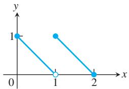
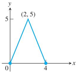
Composition of Functions
In Exercises 39 and 40, find
a.
c.
-
𝑓 ( 𝑥 ) = 1 𝑥 , 𝑔 ( 𝑥 ) = 1 √ 𝑥 + 2 -
𝑓 ( 𝑥 ) = 2 − 𝑥 , 𝑔 ( 𝑥 ) = 3 √ 𝑥 + 1
In Exercises 41 and 42, (a) write formulas for
-
𝑓 ( 𝑥 ) = 2 − 𝑥 2 , 𝑔 ( 𝑥 ) = √ 𝑥 + 2 -
𝑓 ( 𝑥 ) = √ 𝑥 𝑔 ( 𝑥 ) = √ 1 − 𝑥
For Exercises 43 and 44, sketch the graphs of f and
-
𝑓 ( 𝑥 ) = ⎧ { { ⎨ { { ⎩ − 𝑥 − 2 , − 4 ≤ 𝑥 ≤ − 1 − 1 , − 1 < 𝑥 ≤ 1 𝑥 − 2 , 1 < 𝑥 ≤ 2 -
𝑓 ( 𝑥 ) = { 𝑥 + 1 , − 2 ≤ 𝑥 < 0 𝑥 − 1 , 0 ≤ 𝑥 ≤ 2
Composition with absolute values In Exercises 45–52, graph
-
𝑥 -
𝑥 2 | 𝑥 | 2 -
𝑥 3 ∣ 𝑥 3 ∣ -
𝑥 2 + 𝑥 | 𝑥 2 + 𝑥 | -
4 − 𝑥 2 ∣ 4 − 𝑥 2 ∣ -
1 𝑥 1 | 𝑥 | -
√ 𝑥 √ | 𝑥 | -
s i n 𝑥 s i n | 𝑥 |
Shifting and Scaling Graphs
- Suppose the graph of g is given. Write equations for the graphs that are obtained from the graph of g by shifting, scaling, or reflecting, as indicated.
a. Up
b. Down 2 units, left
c. Reflect about the y-axis
d. Reflect about the x-axis
e. Stretch vertically by a factor of 5
f. Compress horizontally by a factor of 5
- Describe how each graph is obtained from the graph of
𝑦 = 𝑓 ( 𝑥 )
a.𝑦 = 𝑓 ( 𝑥 − 5 ) 𝑦 = 𝑓 ( 4 𝑥 ) 𝑦 = 𝑓 ( − 3 𝑥 ) 𝑦 = 𝑓 ( 2 𝑥 + 1 ) 𝑦 = 𝑓 ( 𝑥 3 ) − 4 𝑦 = − 3 𝑓 ( 𝑥 ) + 1 4
In Exercises 55–58, graph each function, not by plotting points, but by starting with the graph of one of the standard functions presented in Figures 1.15–1.17, and applying an appropriate transformation.
-
𝑦 = − √ 1 + 𝑥 2 -
𝑦 = 1 − 𝑥 3 -
𝑦 = 1 2 𝑥 2 + 1 -
𝑦 = ( − 5 𝑥 ) 1 / 3
Trigonometry
In Exercises 59–62, sketch the graph of the given function. What is the period of the function?
-
𝑦 = c o s 2 𝑥 -
𝑦 = s i n 𝑥 2 -
𝑦 = s i n 𝜋 𝑥 -
𝑦 = c o s 𝜋 𝑥 2 -
Sketch the graph
𝑦 = 2 c o s ( 𝑥 − 𝜋 3 ) -
Sketch the graph
𝑦 = 1 + s i n ( 𝑥 + 𝜋 4 )
In Exercises 65–68, ABC is a right triangle with the right angle at C. The sides opposite angles A, B, and C are a, b, and c, respectively.
- a. Find
𝑎 𝑏 𝑐 = 2 𝐵 = 𝜋 / 3
b. Find
- a. Express
𝑎 𝐴 𝑐
b. Express a in terms of A and b.
- a. Express
𝑎 𝐵 𝑏
b. Express c in terms of A and a.
- a. Express
s i n 𝐴
b. Express
-
Height of a pole Two wires stretch from the top T of a vertical pole to points B and C on the ground, where C is 10 m closer to the base of the pole than is B. If wire BT makes an angle of
3 5 ∘ 5 0 ∘ -
Height of a weather balloon Observers at positions A and B 2 km apart simultaneously measure the angle of elevation of a weather balloon to be
4 0 ∘ 7 0 ∘
T 71. a. Graph the function
b. What appears to be the period of this function?
c. Confirm your finding in part (b) algebraically.
T 72. a. Graph
b. What are the domain and range of
c. Is
Transcendental Functions
In Exercises 73–76, find the domain of each function.
-
a.
𝑓 ( 𝑥 ) = 1 + 𝑒 − s i n 𝑥 𝑔 ( 𝑥 ) = 𝑒 𝑥 + l n √ 𝑥 -
a.
𝑓 ( 𝑥 ) = 𝑒 1 / 𝑥 2 𝑔 ( 𝑥 ) = l n | 4 − 𝑥 2 | -
a.
ℎ ( 𝑥 ) = s i n − 1 ( 𝑥 3 ) 𝑓 ( 𝑥 ) = c o s − 1 ( √ 𝑥 − 1 ) -
a.
ℎ ( 𝑥 ) = l n ( c o s − 1 𝑥 ) 𝑓 ( 𝑥 ) = √ 𝜋 − s i n − 1 𝑥 -
If
𝑓 ( 𝑥 ) = l n 𝑥 𝑔 ( 𝑥 ) = 4 − 𝑥 2 𝑓 ∘ 𝑔 , 𝑔 ∘ 𝑓 , 𝑓 ∘ 𝑓 , 𝑔 ∘ 𝑔 -
Determine whether f is even, odd, or neither.
a.
c.
T 79. Graph
T 80. Graph
-
Graph
𝑦 = l n | s i n 𝑥 | 0 ≤ 𝑥 ≤ 2 2 , − 2 ≤ 𝑦 ≤ 0 -
Graph the three functions
𝑦 = 𝑥 𝑎 𝑦 = 𝑎 𝑥 𝑦 = l o g 𝑎 𝑥
Theory and Examples
In Exercises 83 and 84, find the domain and range of each composite function. Then graph the compositions on separate screens. Do the graphs make sense in each case? Give reasons for your answers and comment on any differences you see.
-
a.
𝑦 = s i n − 1 ( s i n 𝑥 ) 𝑦 = s i n ( s i n − 1 𝑥 ) -
a.
𝑦 = c o s − 1 ( c o s 𝑥 ) 𝑦 = c o s ( c o s − 1 𝑥 ) -
Use a graph to decide whether
𝑓
a.
T 86. Use a graph to find to 3 decimal places the values of x for which
- a. Show that
𝑓 ( 𝑥 ) = 𝑥 3 𝑔 ( 𝑥 ) = 3 √ 𝑥
T b. Graph
- a. Show that
ℎ ( 𝑥 ) = 𝑥 3 / 4 𝑘 ( 𝑥 ) = ( 4 𝑥 ) 1 / 3
T b. Graph h and k over an x-interval large enough to show the graphs intersecting at
CHAPTER 1 Additional and Advanced Exercises
Functions and Graphs
-
Are there two functions
𝑓 𝑔 𝑓 ∘ 𝑔 = 𝑔 ∘ 𝑓 -
Are there two functions
𝑓 𝑔 𝑓 𝑔 𝑓 ∘ 𝑔 -
If
𝑓 ( 𝑥 ) 𝑔 ( 𝑥 ) = 𝑓 ( 𝑥 ) − 2 𝑓 -
If
𝑔 ( 𝑥 ) 𝑥 𝑔 ( 0 ) -
Graph the equation
| 𝑥 | + | 𝑦 | = 1 + 𝑥 -
Graph the equation
𝑦 + | 𝑦 | = 𝑥 + | 𝑥 |
Derivations and Proofs
- Prove the following identities.
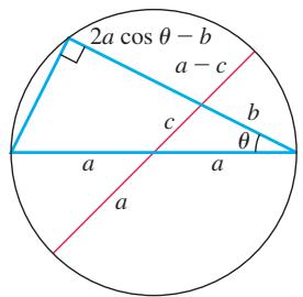
- Explain the following “proof without words” of the law of cosines. (Source: Kung, Sidney H., “Proof Without Words: The Law of Cosines,” Mathematics Magazine, Vol. 63, no. 5, Dec. 1990, p. 342.)
- Show that the area of triangle ABC is given by
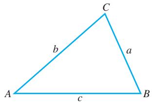
( 1 / 2 ) 𝑎 𝑏 s i n 𝐶 = ( 1 / 2 ) 𝑏 𝑐 s i n 𝐴 = ( 1 / 2 ) 𝑐 𝑎 s i n 𝐵
-
Show that the area of triangle
𝐴 𝐵 𝐶 √ 𝑠 ( 𝑠 − 𝑎 ) ( 𝑠 − 𝑏 ) ( 𝑠 − 𝑐 ) 𝑠 = ( 𝑎 + 𝑏 + 𝑐 ) / 2 -
Show that if
𝑓 𝑓 ( 𝑥 ) = 0 𝑥 𝑓 -
a. Even-odd decompositions Let
𝑓 − 𝑥 𝑥 𝑓
where
b. Uniqueness Show that there is only one way to write
Effects of Parameters on Graphs
- What happens to the graph of
𝑦 = 𝑎 𝑥 2 + 𝑏 𝑥 + 𝑐 𝑎 𝑏 𝑐 𝑏 𝑐 𝑎 ≠ 0 𝑐 𝑏 𝑎 ≠ 0
T 14. What happens to the graph of
Geometry
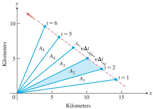
- An object’s center of mass moves at a constant velocity
𝑣 𝐴 1 , 𝐴 2 , … , 𝐴 5
- a. Find the slope of the line from the origin to the midpoint
𝑃 𝐴 𝐵 ( 𝑎 , 𝑏 > 0 )
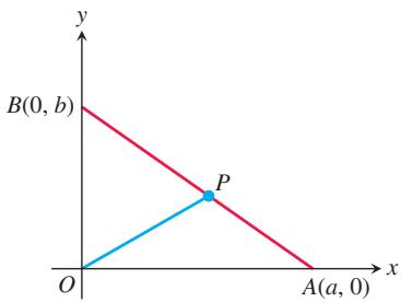
b. When is
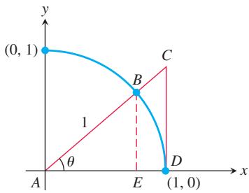
- Consider the quarter-circle of radius 1 and right triangles ABE and ACD given in the accompanying figure. Use standard area formulas to conclude that
- Let
𝑓 ( 𝑥 ) = 𝑎 𝑥 + 𝑏 𝑔 ( 𝑥 ) = 𝑐 𝑥 + 𝑑 𝑎 , 𝑏 , 𝑐 , 𝑑 ( 𝑓 ∘ 𝑔 ) ( 𝑥 ) = ( 𝑔 ∘ 𝑓 ) ( 𝑥 ) 𝑥
Theory and Examples
- Domain and range Suppose that
𝑎 ≠ 0 , 𝑏 ≠ 1 𝑏 > 0
a.
b.
- Inverse functions Let
a. Give a convincing argument that
b. Find a formula for the inverse of
- Depreciation Smith Hauling purchased an 18-wheel truck for
1 0 0 , 0 0 0 . 𝑇 ℎ 𝑒 𝑡 𝑟 𝑢 𝑐 𝑘 𝑑 𝑒 𝑝 𝑟 𝑒 𝑐 𝑖 𝑎 𝑡 𝑒 𝑠 𝑎 𝑡 𝑡 ℎ 𝑒 𝑐 𝑜 𝑛 𝑠 𝑡 𝑎 𝑛 𝑡 𝑟 𝑎 𝑡 𝑒 𝑜 𝑓
a. Write an expression that gives the value y after x years.
b. When is the value of the truck $55,000?
- Drug absorption A drug is administered intravenously for pain. The function
gives the number of units of the drug remaining in the body after t hours.
a. What was the initial number of units of the drug administered?
b. How much is present after 2 hours?
c. Draw the graph of
-
Finding investment time If Juanita invests
1 5 0 0 𝑖 𝑛 𝑎 𝑟 𝑒 𝑡 𝑖 𝑟 𝑒 𝑚 𝑒 𝑛 𝑡 𝑎 𝑐 𝑐 𝑜 𝑢 𝑛 𝑡 𝑡 ℎ 𝑎 𝑡 𝑒 𝑎 𝑟 𝑛 𝑠 8 -
The rule of 70 If you use the approximation
l n 2 ≈ 0 . 7 0 -
For what x > 0 does
𝑥 ( 𝑥 𝑥 ) = ( 𝑥 𝑥 ) 𝑥
T 26. a. If
b. If
Give reasons for your answers.
-
The quotient
( l o g 4 𝑥 ) / ( l o g 2 𝑥 ) -
l o g 𝑥 ( 2 ) l o g 2 ( 𝑥 ) 𝑓 ( 𝑥 ) = l o g 𝑥 ( 2 ) 𝑔 ( 𝑥 ) = l o g 2 ( 𝑥 ) l o g 𝑎 𝑏 = ( l n 𝑏 ) / ( l n 𝑎 ) 𝑓 ( 𝑥 ) 𝑔 ( 𝑥 )
b. Graph f and g together. Comment on the behavior of f in relation to the signs and values of g.
CHAPTER 1 Technology Application Projects
Mathematica/Maple Projects
Projects can be found within MyLab Math.
-
An Overview of Mathematica
- An overview of Mathematica sufficient to complete the Mathematica modules appearing on the Web site.
-
Modeling Change: Springs, Driving Safety, Radioactivity, Trees, Fish, and Mammals Construct and interpret mathematical models, analyze and improve them, and make predictions using them.
Limits and Continuity

OVERVIEW In this chapter we develop the concept of a limit, first intuitively and then formally. We use limits to describe the way a function varies. Some functions vary continuously; small changes in x produce only small changes in