Chapter 2: Limits and Continuity
2.1 Rates of Change and Tangent Lines to Curves
HISTORICAL BIOGRAPHY
Average and Instantaneous Speed
Galileo Galilei
(1564–1642)
Galileo was an Italian mathematician and astronomer. He attempted to apply mathematics to his work in astronomy, physics of kinematics, and strength of materials.
To know more, visit the companion Website.
In the late sixteenth century, Galileo discovered that a solid object dropped from rest (initially not moving) near the surface of the earth and allowed to fall freely, will fall a distance proportional to the square of the time it has been falling. This type of motion is called free fall. It assumes negligible air resistance to slow the object down, and it assumes that gravity is the only force acting on the falling object. If
where 4.9 is the (approximate) constant of proportionality.
More generally, suppose that a moving object has traveled distance
Average Speed
When
Average speed over
EXAMPLE 1 A rock breaks loose from the top of a tall cliff. What is its average speed
(a) during the first 2 seconds of fall?
(b) during the 1-second interval between second 1 and second 2?
Solution The average speed of the rock during a given time interval is the change in distance,
(a) For the first 2 seconds:
(b) From second 1 to second 2:
We want a way to determine the speed of a falling object at a single instant
EXAMPLE 2 Find the speed of the falling rock in Example 1 at t = 1 and t = 2 s.
Solution We can calculate the average speed of the rock over a time interval
We cannot use this formula to calculate the “instantaneous” speed at the exact moment
TABLE 2.1 Average speeds over short time intervals
| Average speed: | ||
| Length of time interval h | Average speed over interval of length h starting at | Average speed over interval of length h starting at |
| 1 | 14.7 | 24.5 |
| 0.1 | 10.29 | 20.09 |
| 0.01 | 9.849 | 19.649 |
| 0.001 | 9.8049 | 19.6049 |
| 0.0001 | 9.80049 | 19.60049 |
The average speed on intervals starting at
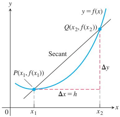
FIGURE 2.1 A secant to the graph
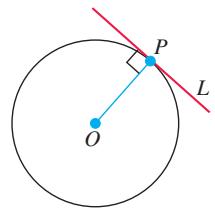
FIGURE 2.2 L is tangent to the circle at P if it passes through P perpendicular to radius OP.
If we set
For values of h different from 0, the expressions on the right and left are equivalent and the average speed is
Similarly, setting
As h gets closer and closer to 0, the average speed has the limiting value 19.6 m/s when
The average speed of a falling object is an example of a more general idea, an average rate of change.
Average Rates of Change and Secant Lines
Given any function
DEFINITION The average rate of change of
with respect to 𝑦 = 𝑓 ( 𝑥 ) over the interval 𝑥 is [ 𝑥 1 , 𝑥 2 ] Δ 𝑦 Δ 𝑥 = 𝑓 ( 𝑥 2 ) − 𝑓 ( 𝑥 1 ) 𝑥 2 − 𝑥 1 = 𝑓 ( 𝑥 1 + ℎ ) − 𝑓 ( 𝑥 1 ) ℎ , ℎ ≠ 0 .
Geometrically, the rate of change of f over
Defining the Slope of a Curve
We know what is meant by the slope of a straight line, which tells us the rate at which it rises or falls—its rate of change as a linear function. But what is meant by the slope of a curve at a point P on the curve? If there were a tangent line to the curve at P—a line that grazes the curve like the tangent line to a circle—it would be reasonable to identify the slope of the tangent line as the slope of the curve at P. We will see that, among all the lines that pass through the point P, the tangent line is the one that gives the best approximation to the curve at P. We need a precise way to specify the tangent line at a point on a curve.
Specifying a tangent line to a circle is straightforward. A line L is tangent to a circle at a point P if L passes through P and is perpendicular to the radius at P (Figure 2.2). But what does it mean to say that a line L is tangent to a more general curve at a point P?
HISTORICAL BIOGRAPHY Pierre de Fermat (1601–1665)
Fermat was born to a prosperous family in France. He studied the classics and mastered Latin, Greek, Italian, and Spanish.
To know more, visit the companion Website.
To define tangency for general curves, we use an approach that analyzes the behavior of the secant lines that pass through P and nearby points Q as Q moves toward P along the curve (Figure 2.3). We start with what we can calculate, namely the slope of the secant line PQ. We then compute the limiting value of the secant line’s slope as Q approaches P along the curve. (We clarify the limit idea in the next section.) If the limit exists, we take it to be the slope of the curve at P and define the tangent line to the curve at P to be the line through P with this slope.
The next example illustrates the geometric idea for finding the tangent line to a curve.
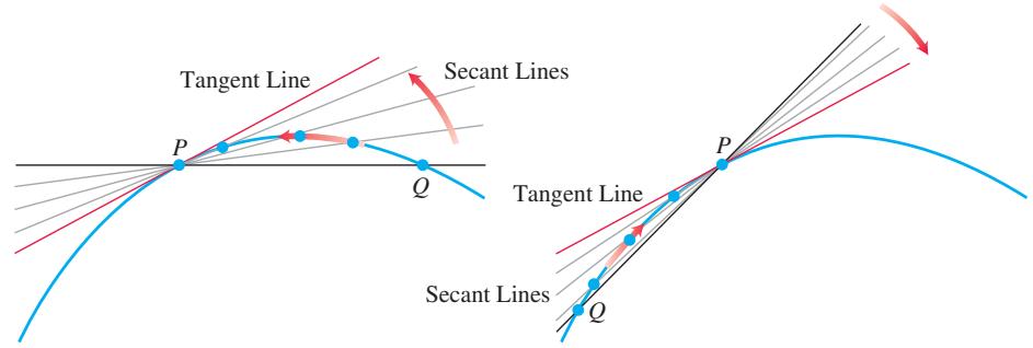
FIGURE 2.3 The tangent line to the curve at P is the line through P whose slope is the limit of the secant line slopes as
EXAMPLE 3 Find the slope of the tangent line to the parabola
Solution We begin with a secant line through
If
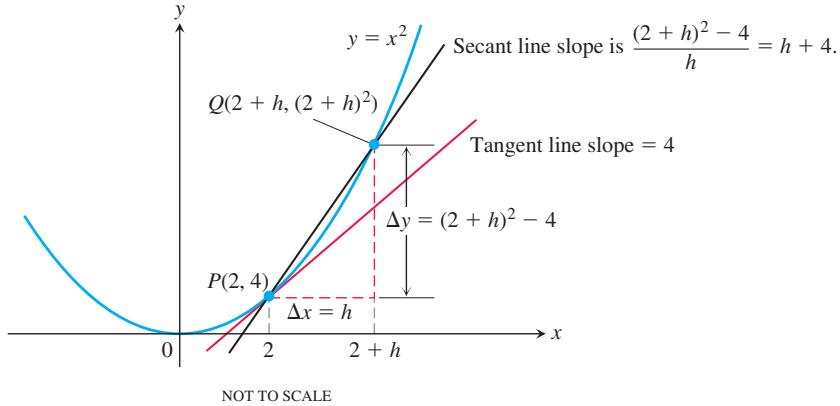
FIGURE 2.4 Finding the slope of the parabola
The tangent line to the parabola at P is the line through P with slope 4:
Rates of Change and Tangent Lines
The rates at which the rock in Example 2 was falling at the instants t = 1 and t = 2 are called instantaneous rates of change. Instantaneous rates of change and slopes of tangent lines are closely connected, as we see in the following examples.
EXAMPLE 4 Figure 2.5 shows how a population p of fruit flies (Drosophila) grew in a 50-day experiment. The flies were counted at regular intervals, the counted values plotted with respect to the number of elapsed days t, and the points joined by a smooth curve (colored blue in Figure 2.5). Find the average growth rate from day 23 to day 45.
Solution There were 150 flies on day 23 and 340 flies on day 45. Thus the number of flies increased by
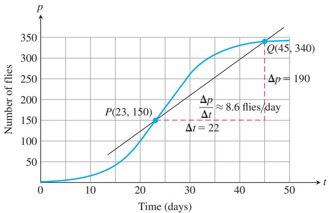
FIGURE 2.5 Growth of a fruit fly population in a controlled experiment. The average rate of change over 22 days is the slope
This average is the slope of the secant line through the points P and Q on the graph in Figure 2.5.
The average rate of change from day 23 to day 45 calculated in Example 4 does not tell us how fast the population was changing on day 23 itself. For that we need to examine time intervals closer to the day in question.
EXAMPLE 5 How fast was the number of flies in the population of Example 4 growing on day 23?
Solution To answer this question, we examine the average rates of change over shorter and shorter time intervals starting at day 23. In geometric terms, we find these rates by calculating the slopes of secant lines from P to Q, for a sequence of points Q approaching P along the curve (Figure 2.6).
| Q | Slope of PQ = Δp/Δt (flies/day) |
| (45,340) | 340 - 150 / 45 - 23 ≈ 8.6 |
| (40,330) | 330 - 150 / 40 - 23 ≈ 10.6 |
| (35,310) | 310 - 150 / 35 - 23 ≈ 13.3 |
| (30,265) | 265 - 150 / 30 - 23 ≈ 16.4 |
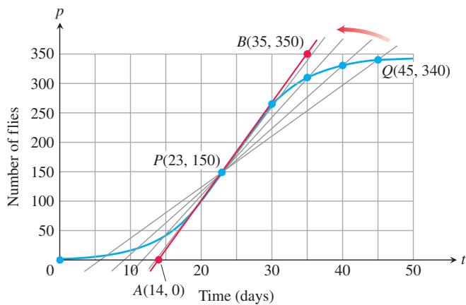
FIGURE 2.6 The positions and slopes of four secant lines through the point P on the fruit fly graph (Example 5).
The values in the table show that the secant line slopes rise from 8.6 to 16.4 as the t-coordinate of Q decreases from 45 to 30, and we would expect the slopes to rise slightly higher as t continued decreasing toward 23. Geometrically, the secant lines rotate counterclockwise about P and seem to approach the red tangent line in the figure. Since the line appears to pass through the points
On day 23 the population was increasing at a rate of about 16.7 flies/day.
The instantaneous rate of change is the value the average rate of change approaches as the length h of the interval over which the change occurs approaches zero. The average rate of change corresponds to the slope of a secant line; the instantaneous rate corresponds to the slope of the tangent line at a fixed value. So instantaneous rates and slopes of tangent lines are closely connected. We give a precise definition for these terms in the next chapter, but to do so we first need to develop the concept of a limit.
EXERCISES 2.1
Average Rates of Change
In Exercises 1–6, find the average rate of change of the function over the given interval or intervals.
Slope of a Curve at a Point
-
𝑓 ( 𝑥 ) = 𝑥 3 + 1 -
𝑔 ( 𝑥 ) = 𝑥 2 − 2 𝑥 -
ℎ ( 𝑡 ) = c o t 𝑡 -
𝑔 ( 𝑡 ) = 2 + c o s 𝑡 -
𝑅 ( 𝜃 ) = √ 4 𝜃 + 1 ; [ 0 , 2 ] -
𝑃 ( 𝜃 ) = 𝜃 3 − 4 𝜃 2 + 5 𝜃 ; [ 1 , 2 ]
In Exercises 7–18, use the method in Example 3 to find (a) the slope of the curve at the given point P, and (b) an equation of the tangent line at P.
a. [2, 3]
b.
-
𝑦 = 𝑥 2 − 5 , 𝑃 ( 2 , − 1 ) -
𝑦 = 7 − 𝑥 2 , 𝑃 ( 2 , 3 )
b.
-
𝑦 = 𝑥 2 − 2 𝑥 − 3 , 𝑃 ( 2 , − 3 ) -
𝑦 = 𝑥 2 − 4 𝑥 , 𝑃 ( 1 , − 3 )
-
𝑦 = 𝑥 3 𝑃 ( 2 , 8 ) -
𝑦 = 2 − 𝑥 3 , 𝑃 ( 1 , 1 )
a.
b.
-
𝑦 = 𝑥 3 − 1 2 𝑥 , 𝑃 ( 1 , − 1 1 ) -
𝑦 = 𝑥 3 − 3 𝑥 2 + 4 , 𝑃 ( 2 , 0 ) -
𝑦 = 1 𝑥 , 𝑃 ( − 2 , − 1 / 2 )

-
𝑦 = 𝑥 2 − 𝑥 , 𝑃 ( 4 , − 2 ) -
𝑦 = √ 𝑥 , 𝑃 ( 4 , 2 ) -
𝑦 = √ 7 − 𝑥 𝑃 ( − 2 , 3 )
Instantaneous Rates of Change
- Speed of a car The accompanying figure shows the time-to-distance graph for a sports car accelerating from a standstill.
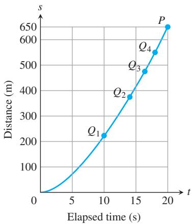
a. Estimate the slopes of secant lines
b. Then estimate the car’s speed at time
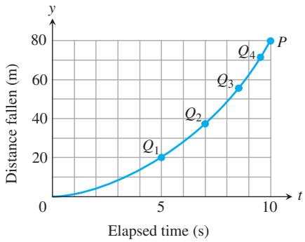
- The accompanying figure shows the plot of distance fallen versus time for an object that fell from the lunar landing module a distance
8 0 m
a. Estimate the slopes of the secant lines
b. About how fast was the object going when it hit the surface?

- The profits of a small company for each of the first five years of its operation are given in the following table:
| Year | Profit in $1000s |
| 2017 | 6 |
| 2018 | 27 |
| 2019 | 62 |
| 2020 | 111 |
| 2021 | 174 |
a. Plot points representing the profit as a function of year, and join them by as smooth a curve as you can.
b. What is the average rate of increase of the profits between 2019 and 2021?
c. Use your graph to estimate the rate at which the profits were changing in 2019.
- Make a table of values for the function
𝐹 ( 𝑥 ) = ( 𝑥 + 2 ) / ( 𝑥 − 2 )
a. Find the average rate of change of
b. Extending the table if necessary, try to determine the rate of change of
T 23. Let
a. Find the average rate of change of
b. Make a table of values of the average rate of change of g with respect to x over the interval
c. What does your table indicate is the rate of change of
T 24. Let
a. Find the average rate of change of
b. Make a table of values of the average rate of change of f with respect to t over the interval
c. What does your table indicate is the rate of change of
- The accompanying graph shows the total distance s traveled by a bicyclist after t hours.
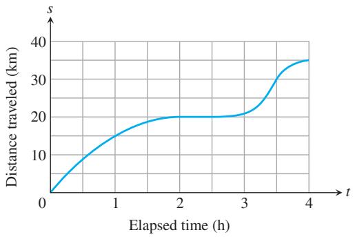
a. Estimate the bicyclist’s average speed over the time intervals [0, 1], [1, 2.5], and [2.5, 3.5].
b. Estimate the bicyclist’s instantaneous speed at the times
c. Estimate the bicyclist’s maximum speed and the specific time at which it occurs.
- The accompanying graph shows the total amount of gasoline A in the gas tank of a motorcycle after being driven for t days.
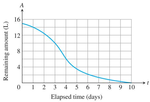
a. Estimate the average rate of gasoline consumption over the time intervals
b. Estimate the instantaneous rate of gasoline consumption at the times t = 1, t = 4, and t = 8.
c. Estimate the maximum rate of gasoline consumption and the specific time at which it occurs.
2.2 Limit of a Function and Limit Laws
HISTORICAL ESSAY
To read this essay, visit the companion Website.
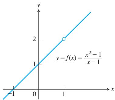
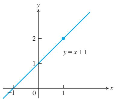
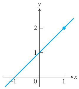
FIGURE 2.7 The graph of f is identical to the line
In Section 2.1 we saw how limits arise when finding the instantaneous rate of change of a function or the tangent line to a curve. We begin this section by presenting an informal definition of the limit of a function. We then describe laws that capture the behavior of limits. These laws enable us to quickly compute limits for a variety of functions, including polynomials and rational functions. We will present the precise definition of a limit in Section 2.3.
Limits of Function Values
Frequently, when studying a function
EXAMPLE 1 How does the function
behave near
Solution The given formula defines f for all real numbers x except x = 1 (since we cannot divide by zero). For any
The graph of f is the line
We will illustrate some other types of behavior near a point in Example 3.
An Informal Description of the Limit of a Function
We now give an informal definition of the limit of a function f at an interior point of the domain of f. Suppose that
TABLE 2.2 As x gets closer to 1,
| x | |
| 0.9 | 1.9 |
| 1.1 | 2.1 |
| 0.99 | 1.99 |
| 1.01 | 2.01 |
| 0.999 | 1.999 |
| 1.001 | 2.001 |
| 0.999999 | 1.999999 |
| 1.000001 | 2.000001 |
(b) Constant function
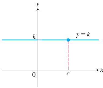
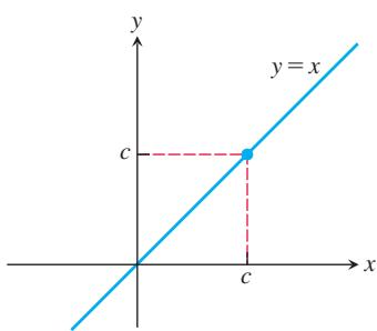
FIGURE 2.9 The functions in Example 3 have limits at all points c.
(a) Identity function
itself. If
This is read “the limit of
Our definition here is informal, because phrases like arbitrarily close and sufficiently close are imprecise; their meaning depends on the context. (To a machinist manufacturing a piston, close may mean within a few hundredths of a millimeter. To an astronomer studying distant galaxies, close may mean within a few thousand light-years.) Nevertheless, the definition is clear enough to enable us to recognize and evaluate limits of many specific functions. We will need the precise definition given in Section 2.3 when we set out to prove theorems about limits or study complicated functions. Here are several more examples exploring the idea of limits.
Essentially, the definition says that the values of
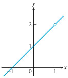
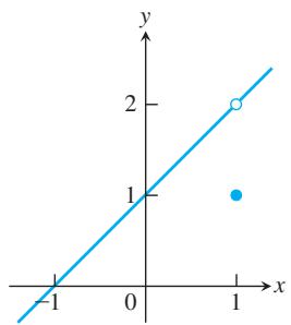
EXAMPLE 2 The limit of a function does not depend on how the function is defined at the point being approached. It does not even matter whether the function is defined at that point. Consider the three functions in Figure 2.8. The function f has limit 2 as
(c)
FIGURE 2.8 The limits of
The process of finding a limit can often be broken up into a series of steps involving limits of basic functions, which are combined using a sequence of simple operations that we will develop. We start with two basic functions.
EXAMPLE 3 We find the limits of the identity function and of a constant function as x approaches x = c.
(a) If
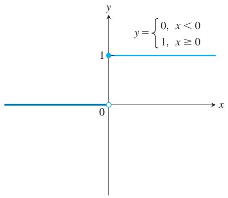
(a) Unit step function
(b) If
For instances of each of these rules we have
Limit of identity function at
and
We prove these rules in Example 3 in Section 2.3.
A function may not have a limit at a particular point. Some ways that limits can fail to exist are illustrated in Figure 2.10 and described in the next example.
(b)
(c)
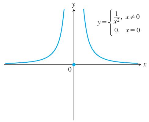
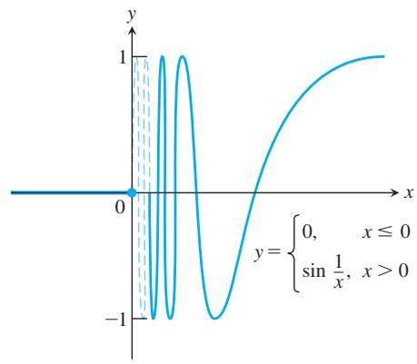
FIGURE 2.10 None of these functions has a limit as x approaches 0 (Example 4).
EXAMPLE 4 Discuss the behavior of the following functions, explaining why they have no limit as
(a)
Solution
(a) This function jumps: The unit step function
(b) This function grows too “large” to have a limit:
| THEOREM 1—Limit Laws | |
| If L, M, c, and k are real numbers and | |
| 1. Sum Rule: | |
| 2. Difference Rule: | |
| 3. Constant Multiple Rule: | |
| 4. Product Rule: | |
| 5. Quotient Rule: | |
| 6. Power Rule: | |
| 7. Root Rule: | |
(c) This function oscillates too much to have a limit:
A function that oscillates may or may not have a limit. In Example 11 we will see a function that oscillates wildly, but nevertheless does have a limit. The problem with the function f discussed in Example 4 is not that it oscillates, but that it oscillates too much for a limit to exist.
The Limit Laws
A few basic rules allow us to break down complicated functions into simple ones when calculating limits. By using these laws, we can greatly simplify many limit computations.
The Sum Rule says that the limit of a sum is the sum of the limits. Similarly, the next rules say that the limit of a difference is the difference of the limits; the limit of a constant times a function is the constant times the limit of the function; the limit of a product is the product of the limits; the limit of a quotient is the quotient of the limits (provided that the limit of the denominator is not 0); the limit of a positive integer power (or root) of a function is the integer power (or root) of the limit (provided that the root of the limit is a real number).
There are simple intuitive arguments for why the properties in Theorem 1 are true (although these do not constitute proofs). If x is sufficiently close to c, then
EXAMPLE 5 Use the observations
(a)
(b)
(c)
Solution
Evaluating Limits of Polynomials and Rational Functions
Theorem 1 simplifies the task of calculating limits of polynomials and rational functions. To evaluate the limit of a polynomial function as x approaches c, just substitute c for x in the formula for the function. To evaluate the limit of a rational function as x approaches a point c at which the denominator is not zero, substitute c for x in the formula for the function. (See Examples 5a and 5b.) We state these results formally as theorems.
THEOREM 3—Limits of Rational Functions
If
EXAMPLE 6 The following calculation illustrates Theorems 2 and 3:
Since the denominator of this rational expression does not equal 0 when we substitute -1 for x, we can just compute the value of the expression at x = -1 to evaluate the limit.
Eliminating Common Factors from Zero Denominators
Theorem 3 applies only if the denominator of the rational function is not zero at the limit point c. If the denominator is zero, canceling common factors in the numerator and
(b)
Identifying Common Factors
If
(a)
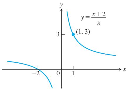
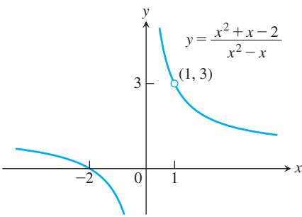
FIGURE 2.11 The graph of
denominator may reduce the fraction to one whose denominator is no longer zero at c. If this happens, we can find the limit by substitution in the simplified fraction.
EXAMPLE 7 Evaluate
Solution We cannot substitute x = 1 because it makes the denominator zero. We test the numerator to see if it, too, is zero at x = 1. It is, so it has a factor of
Using the simpler fraction, we find the limit of these values as
See Figure 2.11.
Using Calculators and Computers to Estimate Limits
We can try using a calculator or computer to guess a limit numerically. However, calculators and computers can sometimes give false values and misleading evidence about limits. Usually the problem is associated with rounding errors, as we now illustrate.
EXAMPLE 8 Estimate the value of
Solution Table 2.3 lists values of the function obtained on a calculator for several points approaching x = 0. As x approaches 0 through the points ±1, ±0.5, ±0.1, and ±0.01, the function seems to approach the number 0.05.
As we take even smaller values of
Is the answer 0.05 or 0, or some other value? We resolve this question in the next example.
Using a computer or calculator may give ambiguous results, as in Example 8. A computer cannot always keep track of enough digits to avoid rounding errors in computing the values of
TABLE 2.3 Computed values of
| x | f(x) |
| ±1 | 0.049876 |
| ±0.5 | 0.049969 |
| ±0.1 | 0.049999 |
| ±0.01 | 0.050000 |
| ±0.0005 | 0.050000 |
| ±0.0001 | 0.000000 |
| ±0.00001 | 0.000000 |
| ±0.000001 | 0.000000 |
EXAMPLE 9 Evaluate
Solution This is the limit we considered in Example 8. We can create a common factor by multiplying both numerator and denominator by the conjugate radical expression
Therefore,
This calculation provides the correct answer, resolving the ambiguous computer results in Example 8.
We cannot always manipulate the terms in an expression to find the limit of a quotient where the denominator becomes zero. In some cases the limit might then be found with geometric arguments (see the proof of Theorem 6 in Section 2.4), or through methods of calculus (developed in Section 4.5). The next theorem shows how to evaluate difficult limits by comparing them with functions having known limits.
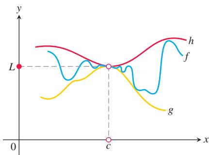
FIGURE 2.12 The graph of f is sandwiched between the graphs of g and h.
The Sandwich Theorem
The following theorem enables us to calculate a variety of limits. It is called the Sandwich Theorem because it refers to a function f whose values are sandwiched between the values of two other functions g and h that have the same limit L at a point c. Being trapped between the values of two functions that approach L, the values of f must also approach L (Figure 2.12). A proof is given in Appendix A.6.
THEOREM 4—The Sandwich Theorem
Suppose that
Then
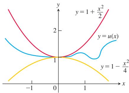
FIGURE 2.13 Any function
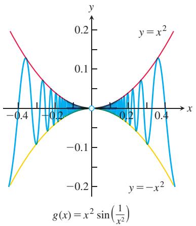
FIGURE 2.14 The graph of the function g (Example 11). It is not defined at x = 0. Even though the function oscillates, it has a limit as
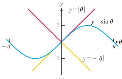
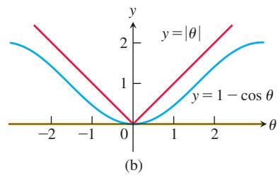
FIGURE 2.15 The Sandwich Theorem confirms the limits in Example 12.
The Sandwich Theorem is also called the Squeeze Theorem or the Pinching Theorem.
EXAMPLE 10 Given a function u that satisfies
find
Solution Since
the Sandwich Theorem implies that
We use the Sandwich Theorem to show that it is possible for a function that oscillates to have a limit.
EXAMPLE 11 How does the function
Solution The formula defines
the Sandwich Theorem implies that
EXAMPLE 12 The Sandwich Theorem helps us establish several important limit rules:
(a)
(b)
(c) For any function
Solution
(a) In Section 1.3 we established that
(b) From Section 1.3,
(c) Since
Example 12 shows that the sine and cosine functions are equal to their limits at
Exercises 2.2
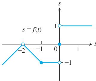
Limits from Graphs
- For the function
𝑔 ( 𝑥 )
a.
- For the function
𝑓 ( 𝑡 )
a.
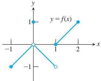
- Which of the following statements about the function
𝑦 = 𝑓 ( 𝑥 )
a.
b.
c.
d.
e.
f.
g.
h.
i.
j.
k.
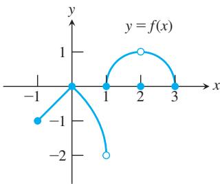
- Which of the following statements about the function
𝑦 = 𝑓 ( 𝑥 )
a.
b.
c.
d.
e.
f.
g.
h.
i.
Existence of Limits
In Exercises 5 and 6, explain why the limits do not exist.
-
l i m 𝑥 → 0 𝑥 | 𝑥 | -
l i m 𝑥 → 1 1 𝑥 − 1 -
Suppose that a function
𝑓 ( 𝑥 ) 𝑥 𝑥 = 𝑐 l i m 𝑥 → 𝑐 𝑓 ( 𝑥 ) -
Suppose that a function
𝑓 ( 𝑥 ) 𝑥 [ − 1 , 1 ] l i m 𝑥 → 0 𝑓 ( 𝑥 ) -
If
l i m 𝑥 → 1 𝑓 ( 𝑥 ) = 5 𝑓 𝑥 = 1 𝑓 ( 1 ) = 5 𝑓 𝑥 = 1 -
If
𝑓 ( 1 ) = 5 l i m 𝑥 → 1 𝑓 ( 𝑥 ) l i m 𝑥 → 1 𝑓 ( 𝑥 ) = 5 l i m 𝑥 → 1 𝑓 ( 𝑥 )
Calculating Limits
Find the limits in Exercises 11–22.
-
l i m 𝑥 → − 3 ( 𝑥 2 − 1 3 ) -
l i m 𝑥 → 2 ( − 𝑥 2 + 5 𝑥 − 2 ) -
l i m 𝑡 → 6 8 ( 𝑡 − 5 ) ( 𝑡 − 7 ) -
l i m 𝑥 → − 2 ( 𝑥 3 − 2 𝑥 2 + 4 𝑥 + 8 ) -
l i m 𝑥 → 2 2 𝑥 + 5 1 1 − 𝑥 3 -
l i m 𝑠 → 2 / 3 ( 8 − 3 𝑠 ) ( 2 𝑠 − 1 ) -
l i m 𝑥 → − 1 / 2 4 𝑥 ( 3 𝑥 + 4 ) 2 -
l i m 𝑦 → 2 𝑦 + 2 𝑦 2 + 5 𝑦 + 6 -
l i m 𝑦 → − 3 ( 5 − 𝑦 ) 4 / 3 -
l i m 𝑧 → 4 √ 𝑧 2 − 1 0 -
l i m ℎ → 0 3 √ 3 ℎ + 1 + 1 -
l i m ℎ → 0 √ 5 ℎ + 4 − 2 ℎ
Limits of quotients Find the limits in Exercises 23–42.
-
l i m 𝑥 → 5 𝑥 − 5 𝑥 2 − 2 5 -
l i m 𝑥 → − 3 𝑥 + 3 𝑥 2 + 4 𝑥 + 3 -
l i m 𝑥 → − 5 𝑥 2 + 3 𝑥 − 1 0 𝑥 + 5 -
l i m 𝑥 → 2 𝑥 2 − 7 𝑥 + 1 0 𝑥 − 2 -
l i m 𝑡 → 1 𝑡 2 + 𝑡 − 2 𝑡 2 − 1 -
l i m 𝑡 → − 1 𝑡 2 + 3 𝑡 + 2 𝑡 2 − 𝑡 − 2 -
l i m 𝑡 → − 2 − 2 𝑥 − 4 𝑥 3 + 2 𝑥 2 -
l i m 𝑦 → 0 5 𝑦 3 + 8 𝑦 2 3 𝑦 4 − 1 6 𝑦 2 -
l i m 𝑥 → 1 𝑥 − 1 − 1 𝑥 − 1 -
l i m 𝑥 → 0 1 𝑥 − 1 + 1 𝑥 + 1 𝑥 -
l i m 𝑢 → 1 𝑢 4 − 1 𝑢 3 − 1 -
l i m 𝑣 → 2 𝑣 3 − 8 𝑣 4 − 1 6 -
l i m 𝑥 → 9 √ 𝑥 − 3 𝑥 − 9 -
l i m 𝑥 → 4 4 𝑥 − 𝑥 2 2 − √ 𝑥 -
l i m 𝑥 → 1 𝑥 − 1 √ 𝑥 + 3 − 2 -
l i m 𝑥 → − 1 √ 𝑥 2 + 8 − 3 𝑥 + 1 -
l i m 𝑥 → 2 √ 𝑥 2 + 1 2 − 4 𝑥 − 2 -
l i m 𝑥 → − 2 𝑥 + 2 √ 𝑥 2 + 5 − 3 -
l i m 𝑥 → − 3 2 − √ 𝑥 2 − 5 𝑥 + 3 -
l i m 𝑥 → 4 4 − 𝑥 5 − √ 𝑥 2 + 9
Limits with trigonometric functions Find the limits in Exercises 43–50.
-
l i m 𝑥 → 0 ( 2 s i n 𝑥 − 1 ) -
l i m 𝑥 → 0 s i n 2 𝑥 -
l i m 𝑥 → 0 s e c 𝑥 -
l i m 𝑥 → 0 t a n 𝑥 -
l i m 𝑥 → 0 1 + 𝑥 + s i n 𝑥 3 c o s 𝑥 -
l i m 𝑥 → 0 ( 𝑥 2 − 1 ) ( 2 − c o s 𝑥 ) -
l i m 𝑥 → − 𝜋 √ 𝑥 + 4 c o s ( 𝑥 + 𝜋 ) -
l i m 𝑥 → 0 √ 7 + s e c 2 𝑥
Using Limit Rules
- Suppose
l i m 𝑥 → 0 𝑓 ( 𝑥 ) = 1 l i m 𝑥 → 0 𝑔 ( 𝑥 ) = − 5
(We assume the denominator is nonzero.)
(b)
(c)
- Let
l i m 𝑥 → 1 ℎ ( 𝑥 ) = 5 l i m 𝑥 → 1 𝑝 ( 𝑥 ) = 1 l i m 𝑥 → 1 𝑟 ( 𝑥 ) = 2
(We assume the denominator is nonzero.)
(b)
(c)
-
Suppose
l i m 𝑥 → 𝑐 𝑓 ( 𝑥 ) = 5 l i m 𝑥 → 𝑐 𝑔 ( 𝑥 ) = − 2 l i m 𝑥 → 𝑐 𝑓 ( 𝑥 ) 𝑔 ( 𝑥 ) l i m 𝑥 → 𝑐 2 𝑓 ( 𝑥 ) 𝑔 ( 𝑥 ) l i m 𝑥 → 𝑐 ( 𝑓 ( 𝑥 ) + 3 𝑔 ( 𝑥 ) ) l i m 𝑥 → 𝑐 𝑓 ( 𝑥 ) 𝑓 ( 𝑥 ) − 𝑔 ( 𝑥 ) -
Suppose
l i m 𝑥 → 4 𝑓 ( 𝑥 ) = 0 l i m 𝑥 → 4 𝑔 ( 𝑥 ) = − 3 l i m 𝑥 → 4 ( 𝑔 ( 𝑥 ) + 3 ) l i m 𝑥 → 4 𝑥 𝑓 ( 𝑥 ) l i m 𝑥 → 4 ( 𝑔 ( 𝑥 ) ) 2 l i m 𝑥 → 4 𝑔 ( 𝑥 ) 𝑓 ( 𝑥 ) − 1 -
Suppose
l i m 𝑥 → 𝑏 𝑓 ( 𝑥 ) = 7 l i m 𝑥 → 𝑏 𝑔 ( 𝑥 ) = − 3 l i m 𝑥 → 𝑏 ( 𝑓 ( 𝑥 ) + 𝑔 ( 𝑥 ) ) l i m 𝑥 → 𝑏 𝑓 ( 𝑥 ) ⋅ 𝑔 ( 𝑥 ) l i m 𝑥 → 𝑏 4 𝑔 ( 𝑥 ) l i m 𝑥 → 𝑏 𝑓 ( 𝑥 ) / 𝑔 ( 𝑥 ) -
Suppose that
l i m 𝑥 → − 2 𝑝 ( 𝑥 ) = 4 , l i m 𝑥 → − 2 𝑟 ( 𝑥 ) = 0 l i m 𝑥 → − 2 𝑠 ( 𝑥 ) = − 3 . l i m 𝑥 → − 2 ( 𝑝 ( 𝑥 ) + 𝑟 ( 𝑥 ) + 𝑠 ( 𝑥 ) ) l i m 𝑥 → − 2 ( 𝑝 ( 𝑥 ) ⋅ 𝑟 ( 𝑥 ) ⋅ 𝑠 ( 𝑥 ) ) l i m 𝑥 → − 2 ( − 4 𝑝 ( 𝑥 ) + 5 𝑟 ( 𝑥 ) ) / 𝑠 ( 𝑥 )
Limits of Average Rates of Change
Because of their connection with secant lines, tangents, and instantaneous rates, limits of the form
occur frequently in calculus. In Exercises 57–62, evaluate this limit for the given value of x and function f.
-
𝑓 ( 𝑥 ) = 𝑥 2 𝑥 = 1 -
𝑓 ( 𝑥 ) = 𝑥 2 𝑥 = − 2 -
𝑓 ( 𝑥 ) = 3 𝑥 − 4 , 𝑥 = 2 -
𝑓 ( 𝑥 ) = 1 / 𝑥 , 𝑥 = − 2 -
𝑓 ( 𝑥 ) = √ 𝑥 , 𝑥 = 7 -
𝑓 ( 𝑥 ) = √ 3 𝑥 + 1 , 𝑥 = 0
Using the Sandwich Theorem
-
If
√ 5 − 2 𝑥 2 ≤ 𝑓 ( 𝑥 ) ≤ √ 5 − 𝑥 2 − 1 ≤ 𝑥 ≤ 1 l i m 𝑥 → 0 𝑓 ( 𝑥 ) -
If
2 − 𝑥 2 ≤ 𝑔 ( 𝑥 ) ≤ 2 c o s 𝑥 𝑥 l i m 𝑥 → 0 𝑔 ( 𝑥 ) -
a. It can be shown that the inequalities
hold for all values of x close to zero (except for x = 0). What, if anything, does this tell you about
Give reasons for your answer.
T b. Graph
- a. Suppose that the inequalities
hold for values of x close to zero, except for x = 0 itself.
(They do, as you will see in Section 16.9.) What, if anything, does this tell you about
Give reasons for your answer.
T b. Graph the equations
Estimating Limits
You will find a graphing calculator useful for Exercises 67–76.
- Let
𝑓 ( 𝑥 ) = ( 𝑥 2 − 9 ) / ( 𝑥 + 3 )
a. Make a table of the values of
b. Support your conclusions in part (a) by graphing f near c = -3 and using Zoom and Trace to estimate y-values on the graph as
c. Find
- Let
𝑔 ( 𝑥 ) = ( 𝑥 2 − 2 ) / ( 𝑥 − √ 2 )
a. Make a table of the values of
b. Support your conclusion in part (a) by graphing g near
c. Find
- Let
𝐺 ( 𝑥 ) = ( 𝑥 + 6 ) / ( 𝑥 2 + 4 𝑥 − 1 2 )
a. Make a table of the values of
b. Support your conclusions in part (a) by graphing
c. Find
- Let
ℎ ( 𝑥 ) = ( 𝑥 2 − 2 𝑥 − 3 ) / ( 𝑥 2 − 4 𝑥 + 3 )
a. Make a table of the values of h at x = 2.9, 2.99, 2.999, and so on. Then estimate
b. Support your conclusions in part (a) by graphing h near c = 3 and using Zoom and Trace to estimate y-values on the graph as
c. Find
- Let
𝑓 ( 𝑥 ) = ( 𝑥 2 − 1 ) / ( | 𝑥 | − 1 )
a. Make tables of the values of
b. Support your conclusion in part (a) by graphing f near c = -1 and using Zoom and Trace to estimate y-values on the graph as
c. Find
- Let
𝐹 ( 𝑥 ) = ( 𝑥 2 + 3 𝑥 + 2 ) / ( 2 − | 𝑥 | )
a. Make tables of values of
b. Support your conclusion in part (a) by graphing
c. Find
- Let
𝑔 ( 𝜃 ) = ( s i n 𝜃 ) / 𝜃
a. Make a table of the values of
b. Support your conclusion in part (a) by graphing g near
- Let
𝐺 ( 𝑡 ) = ( 1 − c o s 𝑡 ) / 𝑡 2
a. Make tables of values of
b. Support your conclusion in part (a) by graphing
- Let
𝑓 ( 𝑥 ) = 𝑥 1 / ( 1 − 𝑥 )
a. Make tables of values of
b. Support your conclusions in part (a) by graphing f near c = 1.
- Let
𝑓 ( 𝑥 ) = ( 3 𝑥 − 1 ) / 𝑥
a. Make tables of values of
b. Support your conclusions in part (a) by graphing
Theory and Examples
-
If
𝑥 4 ≤ 𝑓 ( 𝑥 ) ≤ 𝑥 2 𝑥 [ − 1 , 1 ] 𝑥 2 ≤ 𝑓 ( 𝑥 ) ≤ 𝑥 4 𝑥 < − 1 𝑥 > 1 𝑐 l i m 𝑥 → 𝑐 𝑓 ( 𝑥 ) -
Suppose that
𝑔 ( 𝑥 ) ≤ 𝑓 ( 𝑥 ) ≤ ℎ ( 𝑥 ) 𝑥 ≠ 2
Can we conclude anything about the values of
-
If
l i m 𝑥 → 4 𝑓 ( 𝑥 ) − 5 𝑥 − 2 = 1 l i m 𝑥 → 4 𝑓 ( 𝑥 ) -
If
l i m 𝑥 → − 2 𝑓 ( 𝑥 ) 𝑥 2 = 1 l i m 𝑥 → − 2 𝑓 ( 𝑥 ) l i m 𝑥 → − 2 𝑓 ( 𝑥 ) 𝑥 -
a. If
l i m 𝑥 → 2 𝑓 ( 𝑥 ) − 5 𝑥 − 2 = 3 l i m 𝑥 → 2 𝑓 ( 𝑥 )
b. If
- If
l i m 𝑥 → 0 𝑓 ( 𝑥 ) 𝑥 2 = 1
a.
b.
T 83. a. Graph
b. Confirm your estimate in part (a) with a proof.
T 84. a. Graph
b. Confirm your estimate in part (a) with a proof.
Graphical Estimates of Limits
In Exercises 85–90, use a CAS to perform the following steps:
a. Plot the function near the point c being approached.
b. From your plot, guess the value of the limit.
-
l i m 𝑥 → 2 𝑥 4 − 1 6 𝑥 − 2 -
l i m 𝑥 → − 1 𝑥 3 − 𝑥 2 − 5 𝑥 − 3 ( 𝑥 + 1 ) 2 -
l i m 𝑥 → 0 3 √ 1 + 𝑥 − 1 𝑥 -
l i m 𝑥 → 3 𝑥 2 − 9 √ 𝑥 2 + 7 − 4 -
l i m 𝑥 → 0 1 − c o s 𝑥 𝑥 s i n 𝑥
COMPUTER EXPLORATIONS
l i m 𝑥 → 0 2 𝑥 2 3 − 3 c o s 𝑥
2.3 The Precise Definition of a Limit
We now turn our attention to the precise definition of a limit. The early history of calculus saw controversy about the validity of the basic concepts underlying the theory. Apparent contradictions were argued over by both mathematicians and philosophers. These controversies were resolved by the precise definition, which allows us to replace vague phrases like “gets arbitrarily close to” in the informal definition with specific conditions that can be applied to any particular example. With a rigorous definition, we can avoid misunderstandings, prove the limit properties given in the preceding section, and establish many important limits.
To show that the limit of
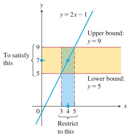
EXAMPLE 1 Consider the function y = 2x - 1 near x = 4. Intuitively it seems clear that y is close to 7 when x is close to 4, so
FIGURE 2.16 Keeping x within 1 unit of x = 4 will keep y within 2 units of y = 7 (Example 1).
Solution We are asked: For what values of
The question then becomes: What values of
Keeping x within 1 unit of x = 4 will keep y within 2 units of y = 7 (Figure 2.16).
In the previous example we determined how close x must be to a particular value c to ensure that the outputs
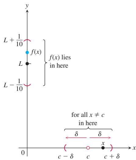
FIGURE 2.17 How should we define
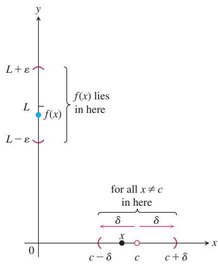
FIGURE 2.18 The relation of
small, by holding x close enough to c. To describe arbitrary prescribed errors, we introduce two constants,
Definition of Limit
Suppose we are watching the values of a function
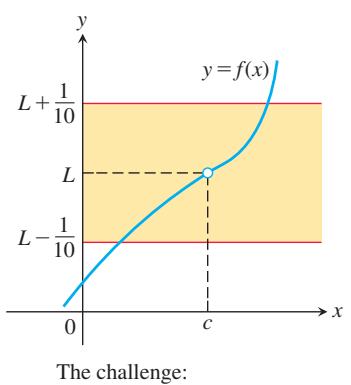
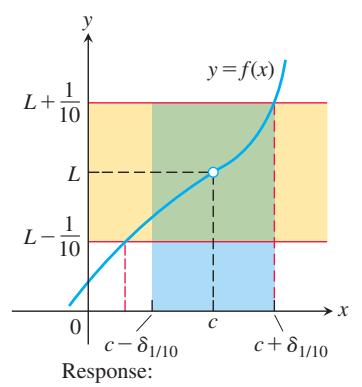
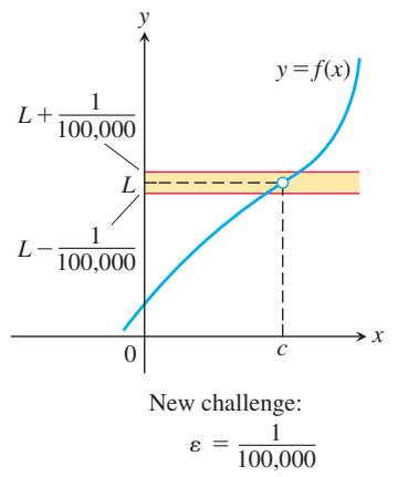
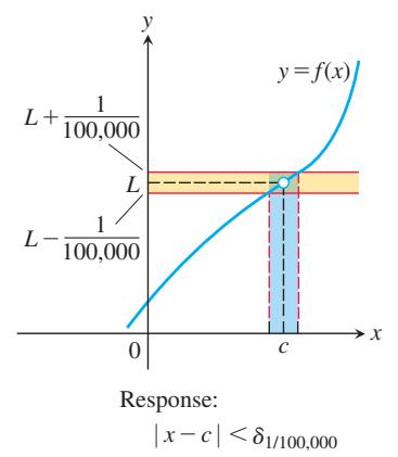
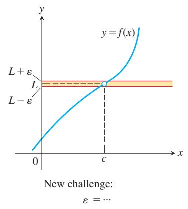
The figures on the next page illustrate the problem. You can think of this as a quarrel between a skeptic and a scholar. The skeptic presents
How do we stop this seemingly endless series of challenges and responses? We can do so by proving that for every error tolerance
DEFINITION Let
be defined on an open interval about 𝑓 ( 𝑥 ) , except possibly at 𝑐 itself. We say that the limit of 𝑐 as 𝑓 ( 𝑥 ) approaches 𝑥 is the number 𝑐 , and write 𝐿 l i m 𝑥 → 𝑐 𝑓 ( 𝑥 ) = 𝐿 , if, for every number
, there exists a corresponding number 𝜀 > 0 such that 𝛿 > 0 | 𝑓 ( 𝑥 ) − 𝐿 | < 𝜀 w h e n e v e r 0 < | 𝑥 − 𝑐 | < 𝛿 .
To visualize the definition, imagine machining a cylindrical shaft to a close tolerance. The diameter of the shaft is determined by turning a dial to a setting measured by a variable x. We try for diameter L, but since nothing is perfect we must be satisfied with a diameter
The definition of limit extends to functions on more general domains. It is only required that each open interval around c contain points in the domain of the function other than c. See Additional and Advanced Exercises 49–53 for examples of limits for functions with complicated domains. In the next section we will see how the definition of limit applies at points lying on the boundary of an interval.
Examples: Testing the Definition
The formal definition of limit does not tell how to find the limit of a function, but it does enable us to verify that a conjectured limit value is correct. The following examples show how the definition can be used to verify limit statements for specific functions. However, the real purpose of the definition is not to do calculations like this, but rather to prove general theorems so that the calculation of specific limits can be simplified, such as the theorems stated in the previous section.
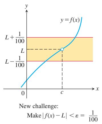
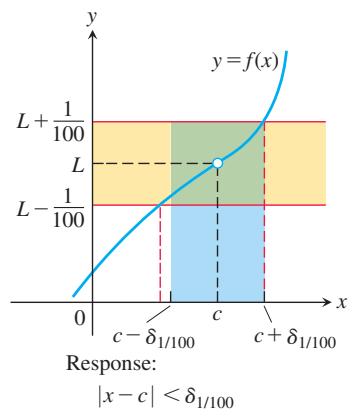
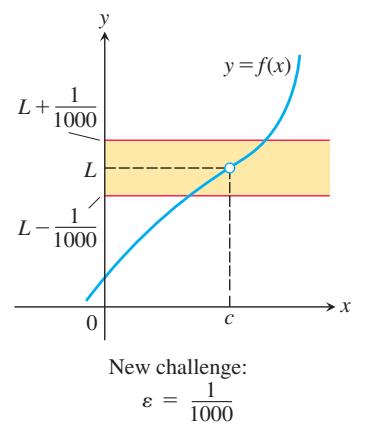
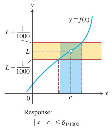
EXAMPLE 2 Show that
Solution Set c = 1,
then
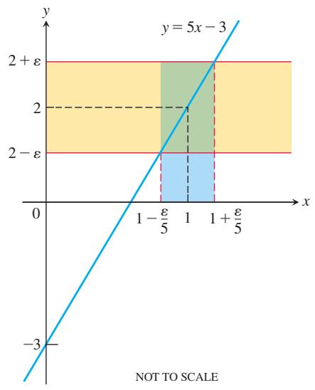
FIGURE 2.19 If
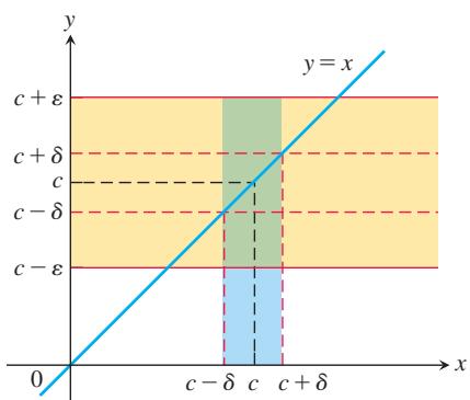
FIGURE 2.20 For the function
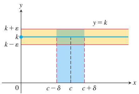
FIGURE 2.21 For the function
We find
Thus, we can take
which proves that
The value of
EXAMPLE 3 Prove the following results, which were presented graphically in Section 2.2.
(a)
(b)
Solution
(a) Let
The implication will hold if
(b) Let
Since k - k = 0, we will always have
Finding Deltas Algebraically for Given Epsilon
In Examples 2 and 3, the interval of values about
EXAMPLE 4 For the limit
Solution We organize the search into two steps.
- Solve the inequality
∣ √ 𝑥 − 1 − 2 ∣ < 1 𝑥 ≠ 5

FIGURE 2.22 An open interval of radius 3 about x = 5 will lie inside the open interval (2,10).
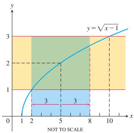
FIGURE 2.23 The function and intervals in Example 4.
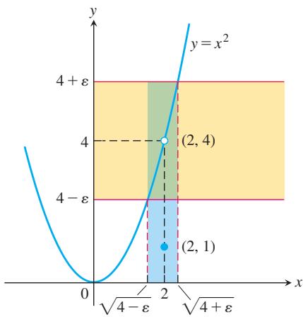
FIGURE 2.24 An interval containing x = 2 so that the function in Example 5 satisfies
The inequality holds for all x in the open interval
- Find a value of
𝛿 > 0 5 − 𝛿 < 𝑥 < 5 + 𝛿 𝛿 = 3 0 < | 𝑥 − 5 | < 𝛿 ∣ √ 𝑥 − 1 − 2 ∣ < 1
How to Find Algebraically a 𝛿 𝑓 , 𝐿 , 𝑐 𝜀 > 0
The process of finding a
can be accomplished in two steps.
-
Solve the inequality
| 𝑓 ( 𝑥 ) − 𝐿 | < 𝜀 ( 𝑎 , 𝑏 ) 𝑥 ≠ 𝑐 -
Find a value of
𝛿 > 0 ( 𝑐 − 𝛿 , 𝑐 + 𝛿 ) ( 𝑎 , 𝑏 ) | 𝑓 ( 𝑥 ) − 𝐿 | < 𝜀 𝑥 ≠ 𝑐 𝛿
EXAMPLE 5 Prove that
Solution Our task is to show that given
- Solve the inequality
| 𝑓 ( 𝑥 ) − 4 | < 𝜀 𝑥 = 2 𝑥 ≠ 2
For
The inequality
- Find a value of
𝛿 > 0 ( 2 − 𝛿 , 2 + 𝛿 ) ( √ 4 − 𝜀 , √ 4 + 𝜀 )
Take
This completes the proof for
If
Using the Definition to Prove Theorems
We do not usually rely on the formal definition of limit to verify specific limits such as those in the preceding examples. Rather, we appeal to general theorems about limits, in particular the theorems of Section 2.2. The definition is used to prove these theorems (Appendix A.6). As an example, we prove part 1 of Theorem 1, the Sum Rule.
EXAMPLE 6 Given that
Solution Let
Regrouping terms, we get
Since
Similarly, since
Let
This shows that
EXERCISES 2.3
Centering Intervals About a Point
In Exercises 1–6, sketch the interval
-
𝑎 = 1 , 𝑏 = 7 , 𝑐 = 5 -
𝑎 = 1 , 𝑏 = 7 , 𝑐 = 2 -
𝑎 = − 7 / 2 , 𝑏 = − 1 / 2 , 𝑐 = − 3 -
𝑎 = − 7 / 2 , 𝑏 = − 1 / 2 , 𝑐 = − 3 / 2 -
𝑎 = 4 / 9 , 𝑏 = 4 / 7 , 𝑐 = 1 / 2 -
𝑎 = 2 . 7 5 9 1 , 𝑏 = 3 . 2 3 9 1 , 𝑐 = 3
Using the Formal Definition
Each of Exercises 31–36 gives a function
Finding Deltas Graphically
In Exercises 7–14, use the graphs to find a
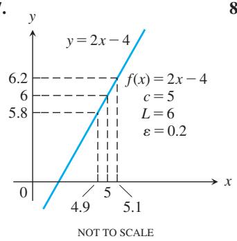
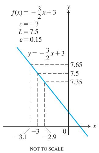
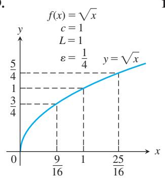
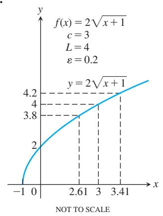
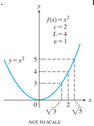
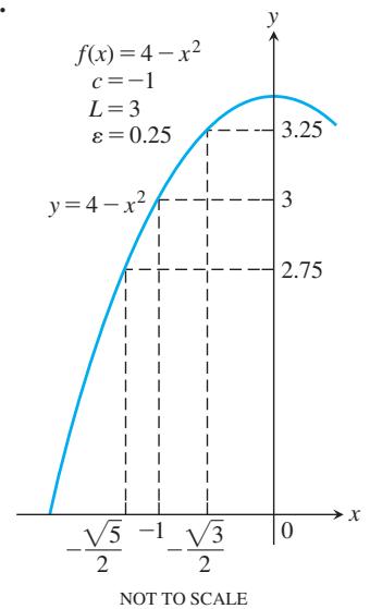
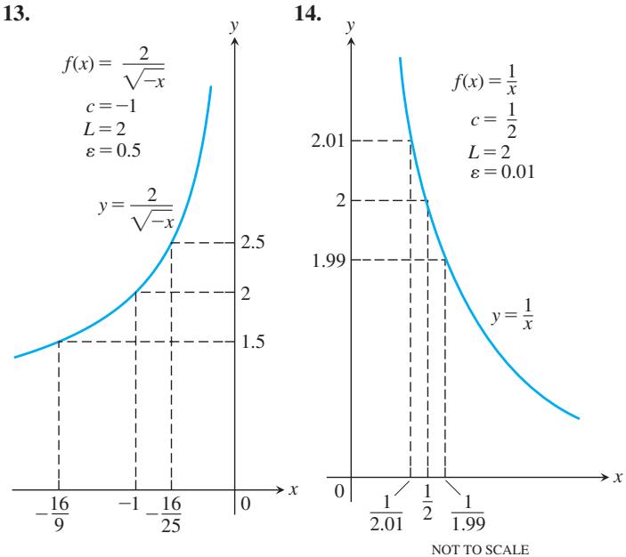
Finding Deltas Algebraically
Each of Exercises 15–30 gives a function
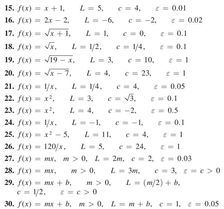
-
𝑓 ( 𝑥 ) = 𝑥 2 + 6 𝑥 + 5 𝑥 + 5 , 𝑐 = − 5 , 𝜀 = 0 . 0 5 -
𝑓 ( 𝑥 ) = √ 1 − 5 𝑥 , 𝑐 = − 3 , 𝜀 = 0 . 5 -
𝑓 ( 𝑥 ) = 4 / 𝑥 𝜀 = 0 . 4
Prove the limit statements in Exercises 37–50.
-
l i m 𝑥 → 4 ( 9 − 𝑥 ) = 5 -
l i m 𝑥 → 3 ( 3 𝑥 − 7 ) = 2 -
l i m 𝑥 → 9 √ 𝑥 − 5 = 2 -
l i m 𝑥 → 0 √ 4 − 𝑥 = 2 -
l i m 𝑥 → 1 𝑓 ( 𝑥 ) = 1 𝑓 ( 𝑥 ) = { 𝑥 2 , 𝑥 ≠ 1 2 , 𝑥 = 1 -
l i m 𝑥 → − 2 𝑓 ( 𝑥 ) = 4 i f 𝑓 ( 𝑥 ) = { 𝑥 2 , 𝑥 ≠ − 2 1 , 𝑥 = − 2 -
l i m 𝑥 → 1 1 𝑥 = 1 -
l i m 𝑥 → √ 3 1 𝑥 2 = 1 3 -
l i m 𝑥 → − 3 𝑥 2 − 9 𝑥 + 3 = − 6 -
l i m 𝑥 → 1 𝑥 2 − 1 𝑥 − 1 = 2 -
l i m 𝑥 → 1 𝑓 ( 𝑥 ) = 2 𝑓 ( 𝑥 ) = { 4 − 2 𝑥 , 𝑥 < 1 6 𝑥 − 4 , 𝑥 ≥ 1 -
l i m 𝑥 → 0 𝑓 ( 𝑥 ) = 0 𝑓 ( 𝑥 ) = { 2 𝑥 , 𝑥 < 0 𝑥 / 2 , 𝑥 ⩾ 0 -
l i m 𝑥 → 0 𝑥 s i n 1 𝑥 = 0
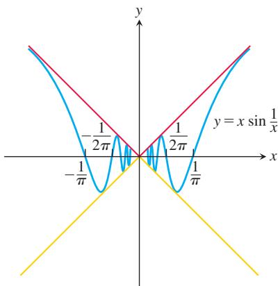
l i m 𝑥 → 0 𝑥 2 s i n 1 𝑥 = 0
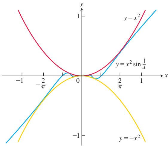
Theory and Examples
-
Define what it means to say that
l i m 𝑥 → 0 𝑔 ( 𝑥 ) = 𝑘 -
Prove that
l i m 𝑥 → 𝑐 𝑓 ( 𝑥 ) = 𝐿 l i m ℎ → 0 𝑓 ( ℎ + 𝑐 ) = 𝐿 -
A wrong statement about limits Show by example that the following statement is wrong.
The number L is the limit of
Explain why the function in your example does not have the given value of L as a limit as
- Another wrong statement about limits Show by example that the following statement is wrong.
The number L is the limit of
-
Grinding engine cylinders Before contracting to grind engine cylinders to a cross-sectional area of
6 0 𝑐 𝑚 2 0 . 1 𝑐 𝑚 2 6 0 𝑐 𝑚 2 𝐴 = 𝜋 ( 𝑥 / 2 ) 2 | 𝐴 − 6 0 | ≤ 0 . 1 -
Manufacturing electrical resistors Ohm’s law for electrical circuits like the one shown in the accompanying figure states that
𝑉 = 𝑅 𝐼 𝑉
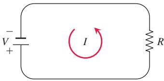
voltage, I is the current in amperes, and R is the resistance in ohms. Your firm has been asked to supply the resistors for a circuit in which V will be 120 volts and I is to be
When Is a Number
In Exercises 57–60 we will consider what it means to not have a limit. Showing L is not a limit We can prove that
We accomplish this for our candidate
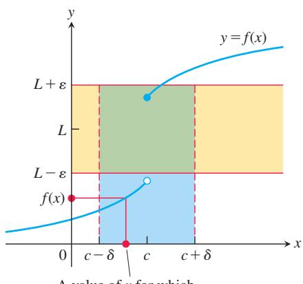
A value of x for which
- Let
𝑓 ( 𝑥 ) = { 𝑥 , 𝑥 < 1 𝑥 + 1 , 𝑥 > 1 .
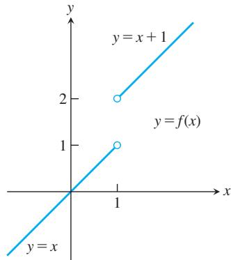
a. Let
That is, show that for each
This will show that
b. Show that
c. Show that
- Let
ℎ ( 𝑥 ) = ⎧ { { ⎨ { { ⎩ 𝑥 2 , 𝑥 < 2 3 , 𝑥 = 3 2 , 𝑥 > 2 .
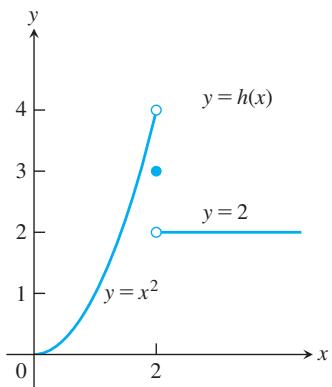
Show that
a.
b.
c.
- For the function graphed here, explain why
a.
l i m 𝑥 → 3 𝑓 ( 𝑥 ) ≠ 4 l i m 𝑥 → 3 𝑓 ( 𝑥 ) ≠ 4 . 8 l i m 𝑥 → 3 𝑓 ( 𝑥 ) ≠ 3
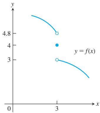
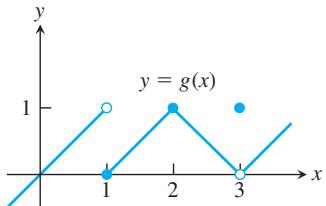
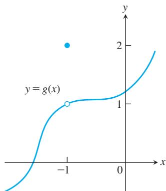
- a. For the function graphed here, show that
l i m 𝑥 → 1 𝑔 ( 𝑥 ) ≠ 2
b. Does
COMPUTER EXPLORATIONS
In Exercises 61–66, you will further explore finding deltas graphically. Use a CAS to perform the following steps:
a. Plot the function
b. Guess the value of the limit L and then evaluate the limit symbolically to see if you guessed correctly.
c. Using the value
d. From your graph in part (c), estimate a
Test your estimate by plotting
e. Repeat parts (c) and (d) successively for
2.4 One-Sided Limits
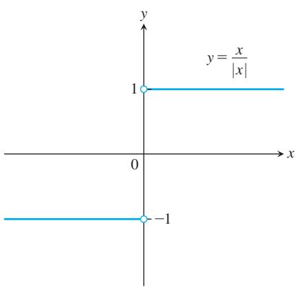
FIGURE 2.25 Different right-hand and left-hand limits at the origin.
In this section we extend the limit concept to one-sided limits, which are limits as x approaches the number c from the left-hand side (where x < c) or the right-hand side (where x > c) only. These allow us to describe functions that have different limits at a point, depending on whether we approach the point from the left or from the right. One-sided limits also allow us to say what it means for a function to have a limit at an endpoint of an interval.
Approaching a Limit from One Side
Suppose a function f is defined on an interval that extends to both sides of a number c. In order for f to have a limit L as x approaches c, the values of
If f fails to have a two-sided limit at c, it may still have a one-sided limit, that is, a limit if the approach is only from one side. If the approach is from the right, the limit is a right-hand limit or limit from the right. Similarly, a left-hand limit is also called a limit from the left.
The function
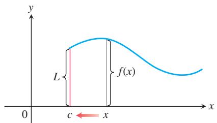
Intuitively, if we consider only the values of
The notation “
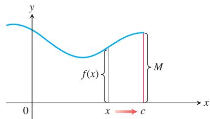
Similarly, if
The symbol “
(a)
(b)
FIGURE 2.26 (a) Right-hand limit as
One-sided limits have all the properties listed in Theorem 1 in Section 2.2. The right-hand limit of the sum of two functions is the sum of their right-hand limits, and so on. The theorems for limits of polynomials and rational functions hold with one-sided limits, as does the Sandwich Theorem. One-sided limits are related to limits at interior points in the following way.
THEOREM 5
Suppose that a function f is defined on an open interval containing c, except perhaps at c itself. Then
Theorem 5 applies at interior points of a function’s domain. At a boundary point of an interval in its domain, a function has a limit when it has an appropriate one-sided limit.
Limits at Endpoints of an Interval
- If
𝑓 ( 𝑏 , 𝑐 ) 𝑐 ( 𝑐 , 𝑑 ) 𝑐
- If
𝑓 ( 𝑐 , 𝑑 ) 𝑐 ( 𝑏 , 𝑐 ) 𝑐
(The definition of a limit on an arbitrary domain is discussed in Additional and Advanced Exercises 39–42.)
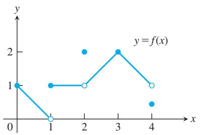
EXAMPLE 1 For the function graphed in Figure 2.27,
FIGURE 2.27 Graph of the function in Example 1.
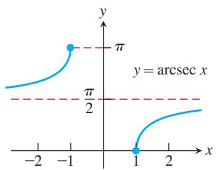
FIGURE 2.28 The arcsec function has limits at
At every other point c in
EXAMPLE 2 The domain of the function arcsec x is a union of the intervals
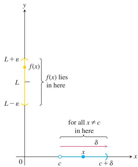
FIGURE 2.29 Intervals associated with the definition of right-hand limit.
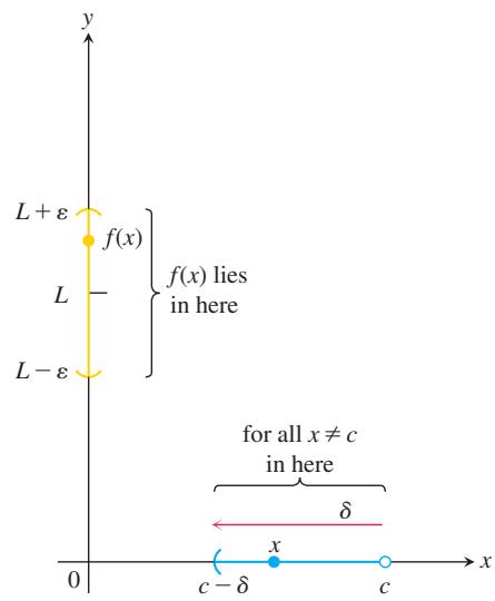
FIGURE 2.30 Intervals associated with the definition of left-hand limit.
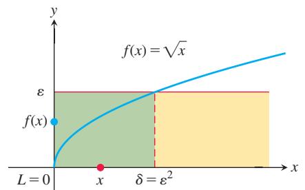
FIGURE 2.31
At every
Precise Definitions of One-Sided Limits
The formal definition of the limit in Section 2.3 is readily modified for one-sided limits.
DEFINITIONS (a) Assume the domain of
contains an interval 𝑓 to the right of ( 𝑐 , 𝑑 ) . We say that 𝑐 has right-hand limit 𝑓 ( 𝑥 ) at 𝐿 , and write 𝑐 l i m 𝑥 → 𝑐 + 𝑓 ( 𝑥 ) = 𝐿 if for every number
there exists a corresponding number 𝜀 > 0 such that 𝛿 > 0 | 𝑓 ( 𝑥 ) − 𝐿 | < 𝜀 w h e n e v e r 𝑐 < 𝑥 < 𝑐 + 𝛿 . (b) Assume the domain of
contains an interval 𝑓 to the left of ( 𝑏 , 𝑐 ) . We say that 𝑐 has left-hand limit 𝑓 at 𝐿 , and write 𝑐 l i m 𝑥 → 𝑐 − 𝑓 ( 𝑥 ) = 𝐿 if for every number
there exists a corresponding number 𝜀 > 0 such that 𝛿 > 0 | 𝑓 ( 𝑥 ) − 𝐿 | < 𝜀 w h e n e v e r 𝑐 − 𝛿 < 𝑥 < 𝑐 .
The definitions are illustrated in Figures 2.29 and 2.30.
EXAMPLE 3 Prove that
Solution Let
or
Squaring both sides of this last inequality gives
If we choose
or
According to the definition, this shows that
Note that since 0 is an endpoint of the domain where
The functions examined so far have had some kind of limit at each point of interest. In general, that need not be the case.
EXAMPLE 4 Show that
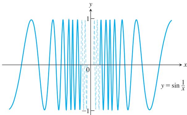
FIGURE 2.32 The function
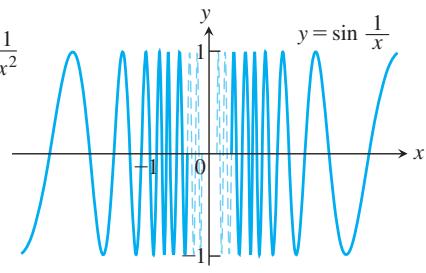
Solution As x approaches zero, its reciprocal, 1/x, grows without bound, and the values of sin (1/x) cycle repeatedly from -1 to 1. There is no single number L that the function’s values stay increasingly close to as x approaches zero. This is true even if we restrict x to positive values or to negative values. The function has neither a right-hand limit nor a left-hand limit at x = 0.
Limits Involving (sin θ)/θ
A central fact about
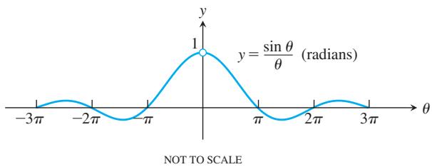
FIGURE 2.33 The graph of
THEOREM 6—Limit of the Ratio sin θ/θ as θ → 0
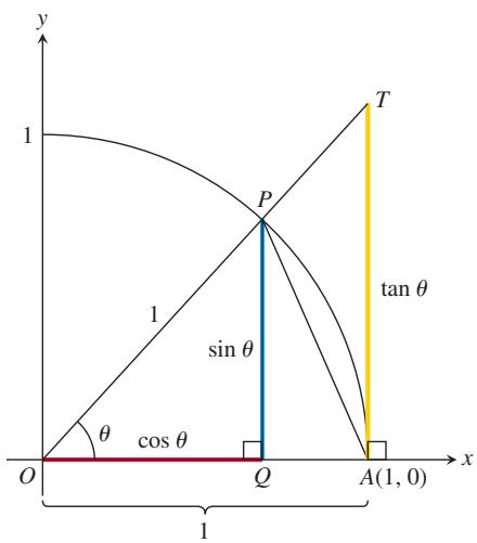
FIGURE 2.34 The ratio TA/OA = tan θ, and OA = 1, so TA = tan θ.
The use of radians to measure angles is essential in Equation (2): The area of sector OAP is
Proof The plan is to show that the right-hand and left-hand limits are both 1. Then we will know that the two-sided limit is 1 as well.
To show that the right-hand limit is 1, we begin with positive values of
Thus,
We can express these areas in terms of
This last inequality goes the same way if we divide all three terms by the number
Taking reciprocals reverses the inequalities:
Since
To consider the left-hand limit, we recall that
so
EXAMPLE 5 Show that (a)
Solution
(a) Using the half-angle formula
(b) Equation (1) does not apply to the original fraction. We need a 2x in the denominator, not a 5x. We produce it by multiplying numerator and denominator by 2/5:
Eq. (1) applies with
EXAMPLE 6 Find
Solution From the definition of tan t and sec 2t, we have
Eq. (1) and Example 12b in Section 2.2
EXAMPLE 7 Show that for nonzero constants A and B.
Solution
EXERCISES 2.4
Finding Limits Graphically
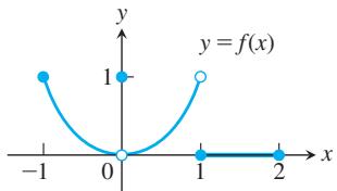
- Which of the following statements about the function
𝑦 = 𝑓 ( 𝑥 )
a.
- Which of the following statements about the function
𝑦 = 𝑓 ( 𝑥 )
c.
e.
f.
g.
h.
i.
j.
k.
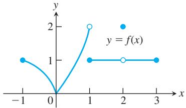
a.
c.
d.
e.
g.
h.
i.
j.
- Let
𝑓 ( 𝑥 ) = { 3 − 𝑥 , 𝑥 < 2 𝑥 2 + 1 , 𝑥 > 2 .
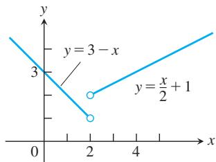
a. Find
b. Does
c. Find
d. Does
- Let
𝑓 ( 𝑥 ) = ⎧ { { ⎨ { { ⎩ 3 − 𝑥 , 𝑥 < 2 2 , 𝑥 = 2 𝑥 2 , 𝑥 > 2 .
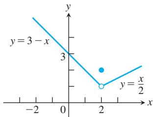
a. Find
b. Does
c. Find
d. Does
- Let
𝑓 ( 𝑥 ) = { 0 , 𝑥 ≤ 0 s i n 1 𝑥 , 𝑥 > 0 .
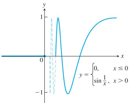
a. Does
b. Does
c. Does
- Let
𝑔 ( 𝑥 ) = √ 𝑥 s i n ( 1 / 𝑥 )
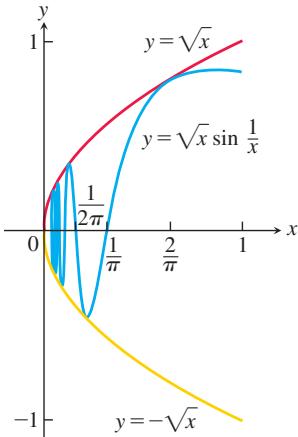
a. Does
b. Does
c. Does
- a. Graph
𝑓 ( 𝑥 ) = { 𝑥 3 , 𝑥 ≠ 1 0 , 𝑥 = 1 .
b. Find
c. Does
- a. Graph
𝑓 ( 𝑥 ) = { 1 − 𝑥 2 , 𝑥 ≠ 1 2 , 𝑥 = 1 .
b. Find
c. Does
Graph the functions in Exercises 9 and 10. Then answer these questions.
a. What are the domain and range of
b. At what points
c. At what points does the left-hand limit exist but not the right-hand limit?
d. At what points does the right-hand limit exist but not the left-hand limit?
Finding One-Sided Limits Algebraically Find the limits in Exercises 11–20.
-
l i m 𝑥 → − 0 . 5 − √ 𝑥 + 2 𝑥 + 1 -
l i m 𝑥 → 1 + √ 𝑥 − 1 𝑥 + 2 -
l i m 𝑥 → − 2 + ( 𝑥 𝑥 + 1 ) ( 2 𝑥 + 5 𝑥 2 + 𝑥 ) -
l i m 𝑥 → 1 − ( 1 𝑥 + 1 ) ( 𝑥 + 6 𝑥 ) ( 3 − 𝑥 7 ) -
l i m ℎ → 0 + √ ℎ 2 + 4 ℎ + 5 − √ 5 ℎ -
l i m ℎ → 0 − √ 6 − √ 5 ℎ 2 + 1 1 ℎ + 6 ℎ -
a.
l i m 𝑥 → − 2 + ( 𝑥 + 3 ) | 𝑥 + 2 | 𝑥 + 2 l i m 𝑥 → − 2 − ( 𝑥 + 3 ) | 𝑥 + 2 | 𝑥 + 2 -
a.
l i m 𝑥 → 1 + √ 2 𝑥 ( 𝑥 − 1 ) | 𝑥 − 1 |
b.
- a.
l i m 𝑥 → 0 + | s i n 𝑥 | 𝑥
b.
- a.
l i m 𝑥 → 0 + 1 − c o s 𝑥 | c o s 𝑥 − 1 |
b.
Use the graph of the greatest integer function
- a.
l i m 𝜃 → 3 + ⌊ 𝜃 ⌋ 𝜃
- a.
l i m 𝑡 → 4 + ( 𝑡 − ⌊ 𝑡 ⌋ ) l i m 𝑡 → 4 − ( 𝑡 − ⌊ 𝑡 ⌋ )
Using
Find the limits in Exercises 23–46.
-
l i m 𝜃 → 0 s i n √ 2 𝜃 √ 2 𝜃 -
l i m 𝑡 → 0 s i n 𝑘 𝑡 𝑡 -
l i m 𝑦 → 0 s i n 3 𝑦 4 𝑦 -
l i m ℎ → 0 − ℎ s i n 3 ℎ -
l i m 𝑥 → 0 t a n 2 𝑥 𝑥 -
l i m 𝑡 → 0 2 𝑡 t a n 𝑡 -
l i m 𝑥 → 0 𝑥 c s c 2 𝑥 c o s 5 𝑥 -
l i m 𝑥 → 0 6 𝑥 2 ( c o t 𝑥 ) ( c s c 2 𝑥 ) -
l i m 𝑥 → 0 𝑥 + 𝑥 c o s 𝑥 s i n 𝑥 c o s 𝑥 -
l i m 𝑥 → 0 𝑥 2 − 𝑥 + s i n 𝑥 2 𝑥 -
l i m 𝜃 → 0 1 − c o s 𝜃 s i n 2 𝜃 -
l i m 𝑥 → 0 𝑥 − 𝑥 c o s 𝑥 s i n 2 3 𝑥 -
l i m 𝑡 → 0 s i n ( 1 − c o s 𝑡 ) 1 − c o s 𝑡 -
l i m ℎ → 0 s i n ( s i n ℎ ) s i n ℎ -
l i m 𝜃 → 0 s i n 𝜃 s i n 2 𝜃 -
l i m 𝑥 → 0 s i n 5 𝑥 s i n 4 𝑥 -
l i m 𝜃 → 0 𝜃 c o s 𝜃 -
l i m 𝜃 → 0 s i n 𝜃 c o t 2 𝜃 -
l i m 𝑥 → 0 t a n 3 𝑥 s i n 8 𝑥 -
l i m 𝑦 → 0 s i n 3 𝑦 c o t 5 𝑦 𝑦 c o t 4 𝑦 -
l i m 𝜃 → 0 t a n 𝜃 𝜃 2 c o t 3 𝜃 -
l i m 𝜃 → 0 𝜃 c o t 4 𝜃 s i n 2 𝜃 c o t 2 2 𝜃 -
l i m 𝑥 → 0 1 − c o s 3 𝑥 2 𝑥 -
l i m 𝑥 → 0 c o s 2 𝑥 − c o s 𝑥 𝑥 2
Theory and Examples
-
Once you know
l i m 𝑥 → 𝑎 + 𝑓 ( 𝑥 ) l i m 𝑥 → 𝑎 − 𝑓 ( 𝑥 ) l i m 𝑥 → 𝑎 𝑓 ( 𝑥 ) -
If you know that
l i m 𝑥 → 𝑐 𝑓 ( 𝑥 ) l i m 𝑥 → 𝑐 + 𝑓 ( 𝑥 ) -
Suppose that
𝑓 𝑥 l i m 𝑥 → 0 + 𝑓 ( 𝑥 ) = 3 l i m 𝑥 → 0 − 𝑓 ( 𝑥 ) -
Suppose that
𝑓 𝑥 l i m 𝑥 → 2 − 𝑓 ( 𝑥 ) = 7 l i m 𝑥 → − 2 − 𝑓 ( 𝑥 ) l i m 𝑥 → − 2 + 𝑓 ( 𝑥 )
Formal Definitions of One-Sided Limits
-
Given
𝜀 > 0 𝐼 = ( 5 , 5 + 𝛿 ) 𝛿 > 0 𝑥 𝐼 √ 𝑥 − 5 < 𝜀 -
Given
𝜀 > 0 𝐼 = ( 4 − 𝛿 , 4 ) 𝛿 > 0 𝑥 𝐼 √ 4 − 𝑥 < 𝜀
Use the definitions of right-hand and left-hand limits to prove the limit statements in Exercises 53 and 54.
-
l i m 𝑥 → 0 − 𝑥 | 𝑥 | = − 1 -
l i m 𝑥 → 2 + 𝑥 − 2 | 𝑥 − 2 | = 1 -
Greatest integer function Find (a)
l i m 𝑥 → 4 0 0 + ⌊ 𝑥 ⌋ l i m 𝑥 → 4 0 0 − ⌊ 𝑥 ⌋ l i m 𝑥 → 4 0 0 ⌊ 𝑥 ⌋ -
One-sided limits Let
𝑓 ( 𝑥 ) = { 𝑥 2 s i n ( 1 / 𝑥 ) , 𝑥 < 0 √ 𝑥 , 𝑥 > 0 . l i m 𝑥 → 0 + 𝑓 ( 𝑥 ) l i m 𝑥 → 0 − 𝑓 ( 𝑥 ) l i m 𝑥 → 0 𝑓 ( 𝑥 )
2.5 Limits Involving Infinity; Asymptotes of Graphs
In this section we investigate the behavior of a function when the magnitude of the independent variable x becomes increasingly large, or
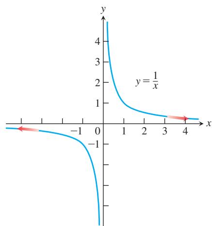
FIGURE 2.35 The graph of
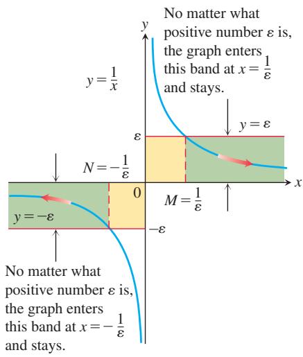
FIGURE 2.36 The geometry behind the argument in Example 1.
Finite Limits as 𝑥 → ± ∞
The symbol for infinity
DEFINITIONS
- We say that
has the limit 𝑓 ( 𝑥 ) as 𝐿 approaches infinity and write 𝑥 l i m 𝑥 → ∞ 𝑓 ( 𝑥 ) = 𝐿 if, for every number
, there exists a corresponding number 𝜀 > 0 such that for all 𝑀 in the domain of 𝑥 𝑓 | 𝑓 ( 𝑥 ) − 𝐿 | < 𝜀 w h e n e v e r 𝑥 > 𝑀 .
- We say that
has the limit L as x approaches negative infinity and write 𝑓 ( 𝑥 ) l i m 𝑥 → − ∞ 𝑓 ( 𝑥 ) = 𝐿 if, for every number
, there exists a corresponding number 𝜀 > 0 such that for all 𝑁 in the domain of 𝑥 𝑓 | 𝑓 ( 𝑥 ) − 𝐿 | < 𝜀 w h e n e v e r 𝑥 < 𝑁 .
Intuitively,
The strategy for calculating limits of functions as
The basic facts to be verified by applying the formal definition are
We prove the second result in Example 1, and leave the first to Exercises 93 and 94.
EXAMPLE 1 Show that
Solution
(a) Let
The implication will hold if
(a)
(a)
(b) Let
The implication will hold if
Limits at infinity have properties similar to those of finite limits.
THEOREM 7
All the Limit Laws in Theorem 1 are true when we replace
EXAMPLE 2 The properties in Theorem 7 are used to calculate limits in the same way as when x approaches a finite number c.
Sum Rule
Known limits
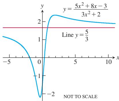
FIGURE 2.37 The graph of the function in Example 3a. The graph approaches the line y = 5/3 as |x| increases.
Limits at Infinity of Rational Functions
To determine the limit of a rational function as
EXAMPLE 3 These examples illustrate what happens when the degree of the numerator is less than or equal to the degree of the denominator.
Cases for which the degree of the numerator is greater than the degree of the denominator are illustrated in Examples 10 and 14.
Horizontal Asymptotes
If the distance between the graph of a function and some fixed line approaches zero as a point on the graph moves increasingly far from the origin, we say that the graph approaches the line asymptotically and that the line is an asymptote of the graph.
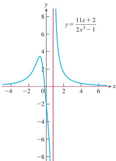
FIGURE 2.38 The graph of the function in Example 3b. The graph approaches the x-axis as
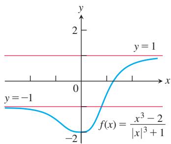
FIGURE 2.39 The graph of the function in Example 4 has two horizontal asymptotes.
Looking at
and on the left because
We say that the x-axis is a horizontal asymptote of the graph of
DEFINITION A line
is a horizontal asymptote of the graph of a function 𝑦 = 𝑏 if either 𝑦 = 𝑓 ( 𝑥 ) l i m 𝑥 → ∞ 𝑓 ( 𝑥 ) = 𝑏 o r l i m 𝑥 → − ∞ 𝑓 ( 𝑥 ) = 𝑏 .
The graph of a function can have zero, one, or two horizontal asymptotes, depending on whether the function has limits as
The graph of the function
sketched in Figure 2.37 (Example 3a) has the line y = 5/3 as a horizontal asymptote on both the right and the left because
EXAMPLE 4 Find the horizontal asymptotes of the graph of
Solution We calculate the limits as
The horizontal asymptotes are y = -1 and y = 1. The graph is displayed in Figure 2.39. Notice that the graph crosses the horizontal asymptote y = -1 for a positive value of x.
EXAMPLE 5 The x-axis (the line y = 0) is a horizontal asymptote of the graph of
To see this, we use the definition of a limit as
Now
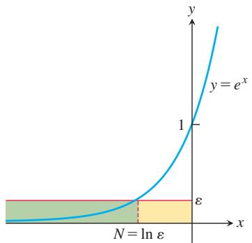
FIGURE 2.40 The graph of
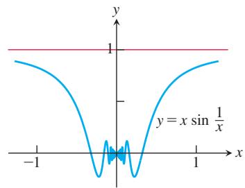
FIGURE 2.41 The line y = 1 is a horizontal asymptote of the function graphed here (Example 6b).
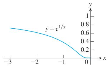
FIGURE 2.42 The graph of
Let
Sometimes it is helpful to transform a limit in which x approaches
EXAMPLE 6 Find (a)
Solution
(a) We introduce the new variable
(b) We calculate the limits as
The graph is shown in Figure 2.41, and we see that the line
Similarly, we can investigate the behavior of
EXAMPLE 7
Solution We let
(Figure 2.42).
The Sandwich Theorem also holds for limits as
EXAMPLE 8 Using the Sandwich Theorem, find the horizontal asymptote of the curve
Solution We are interested in the behavior as
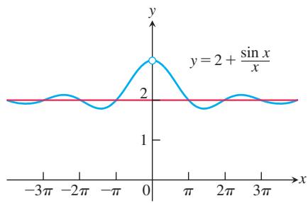
FIGURE 2.43 A curve may cross one of its asymptotes infinitely often (Example 8).
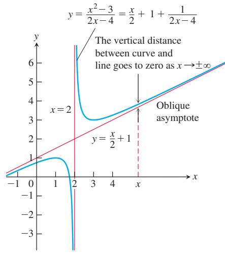
FIGURE 2.44 The graph of the function in Example 10 has an oblique asymptote.
and
and the line y = 2 is a horizontal asymptote of the curve on both left and right (Figure 2.43).
This example illustrates that a curve may cross one of its horizontal asymptotes many times.
Solution Both of the terms x and
As
Oblique Asymptotes
If the degree of the numerator of a rational function is 1 greater than the degree of the denominator, the graph has an oblique or slant line asymptote. We find an equation for the asymptote by dividing numerator by denominator to express f as a linear function plus a remainder that goes to zero as
EXAMPLE 10 Find the oblique asymptote of the graph of
in Figure 2.44.
Solution We are interested in the behavior as
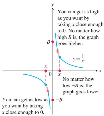
FIGURE 2.45 One-sided infinite limits:
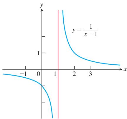
FIGURE 2.46 Near x = 1, the function
This tells us that
As
an asymptote of the graph of
Notice in Example 10 that if the degree of the numerator in a rational function is greater than the degree of the denominator, then the limit as
Infinite Limits
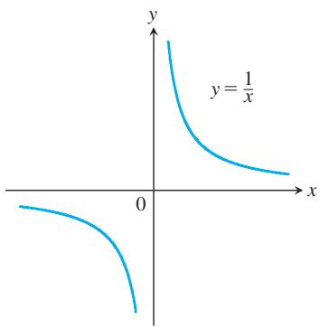
Let us look again at the function
Thus, f has no limit as
In writing this equation, we are not saying that the limit exists. Nor are we saying that there is a real number
As
Again, we are not saying that the limit exists and equals the number
Geometric Solution The graph of
Analytic Solution Think about the number x - 1 and its reciprocal. As
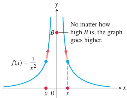
EXAMPLE 12 Discuss the behavior of
Solution As x approaches zero from either side, the values of
) in The function
EXAMPLE 13 These examples illustrate that rational functions can behave in various ways near zeros of the denominator.
Can substitute 2 for x after algebraic manipulation eliminates division by 0.
Again substitute 2 for x after algebraic manipulation eliminates division by 0.
The values are negative for
The values are positive for
Limits from left and from right differ.
Denominator is positive, so values are negative near x = 2.
In parts (a) and (b), the effect of the zero in the denominator at x = 2 is canceled because the numerator is zero there also. Thus a finite limit exists. This is not true in part (f), where cancellation still leaves a zero factor in the denominator.
Solution We are asked to find the limit of a rational function as
because the numerator tends to
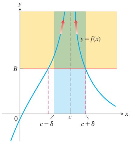
FIGURE 2.48 For
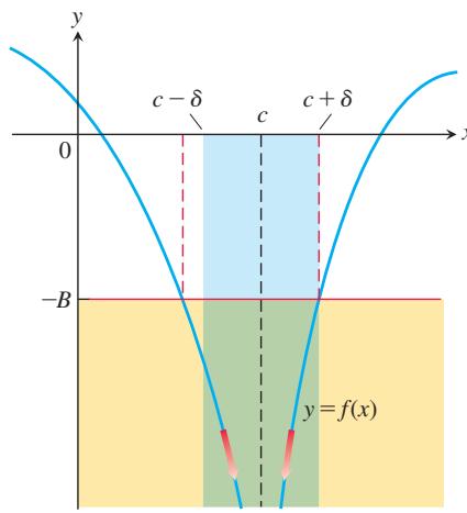
FIGURE 2.49 For
Precise Definitions of Infinite Limits
Instead of requiring
DEFINITIONS
- We say that
approaches infinity as 𝑓 ( 𝑥 ) approaches 𝑥 , and write 𝑐 l i m 𝑥 → 𝑐 𝑓 ( 𝑥 ) = ∞ , if for every positive real number B there exists a corresponding
such that 𝛿 > 0 𝑓 ( 𝑥 ) > 𝐵 w h e n e v e r 0 < | 𝑥 − 𝑐 | < 𝛿 .
- We say that
approaches negative infinity as x approaches c, and write 𝑓 ( 𝑥 ) l i m 𝑥 → 𝑐 𝑓 ( 𝑥 ) = − ∞ , if for every negative real number -B there exists a corresponding
such that 𝛿 > 0 𝑓 ( 𝑥 ) < − 𝐵 w h e n e v e r 0 < | 𝑥 − 𝑐 | < 𝛿 .
The precise definitions of one-sided infinite limits at
EXAMPLE 15 Prove that
Solution Given B > 0, we want to find
Now,
or, equivalently,
Thus, choosing
Therefore, by definition,
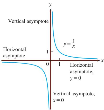
FIGURE 2.50 The coordinate axes are asymptotes of both branches of the hyperbola
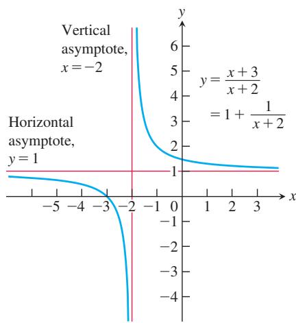
FIGURE 2.51 The lines y = 1 and x = -2 are asymptotes of the curve in Example 16.
Vertical Asymptotes
Notice that the distance between a point on the graph of
We say that the line x = 0 (the y-axis) is a vertical asymptote of the graph of
DEFINITION A line
is a vertical asymptote of the graph of a function 𝑥 = 𝑎 if either 𝑦 = 𝑓 ( 𝑥 ) l i m 𝑥 → 𝑎 + 𝑓 ( 𝑥 ) = ± ∞ o r l i m 𝑥 → 𝑎 − 𝑓 ( 𝑥 ) = ± ∞ .
EXAMPLE 16 Find the horizontal and vertical asymptotes of the curve
Solution We are interested in the behavior as
The asymptotes are revealed if we recast the rational function as a polynomial with a remainder, by dividing
This result enables us to rewrite
We see that the curve in question is the graph of
EXAMPLE 17 Find the horizontal and vertical asymptotes of the graph of
Solution We are interested in the behavior as
(a) The behavior as
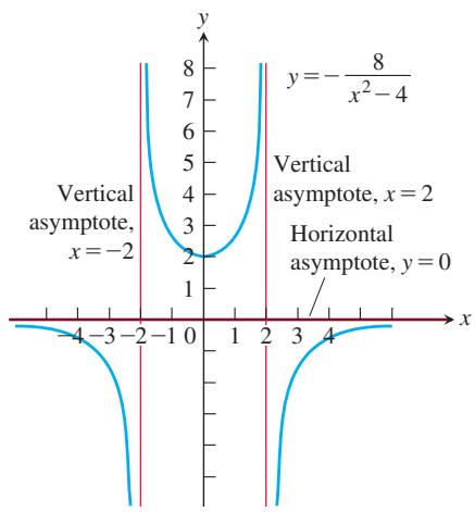
FIGURE 2.52 Graph of the function in Example 17. Notice that the curve approaches the x-axis from only one side. Asymptotes do not have to be two-sided.
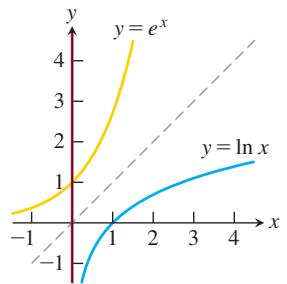
FIGURE 2.53 The vertical line x = 0 is a vertical asymptote of the natural logarithm function (Example 18).
(b) The behavior as
the line x = 2 is a vertical asymptote both from the right and from the left. By symmetry, the line x = -2 is also a vertical asymptote.
There are no other asymptotes because f has a finite limit at all other points.
EXAMPLE 18 The graph of the natural logarithm function has the y-axis (the line x = 0) as a vertical asymptote. We see this from the graph sketched in Figure 2.53 (which is the reflection of the graph of the natural exponential function across the line y = x) and the fact that the x-axis is a horizontal asymptote of
The same result is true for
EXAMPLE 19 The curves
both have vertical asymptotes at odd-integer multiples of
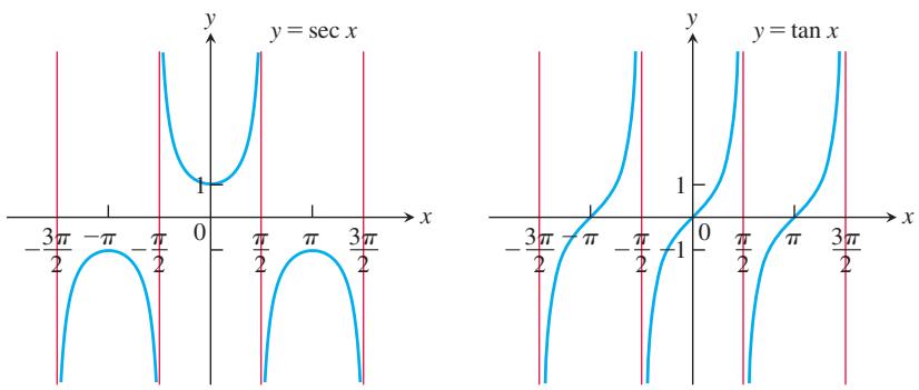
FIGURE 2.54 The graphs of sec x and tan x have infinitely many vertical asymptotes (Example 19).
Dominant Terms
In Example 10 we saw that by using long division, we can rewrite the function
as a linear function plus a remainder term:
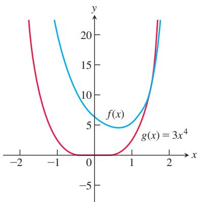
(a)
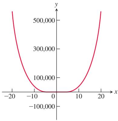
(b)
FIGURE 2.55 The graphs of f and g are (a) distinct for
This tells us immediately that
For
For
If we want to know how f behaves, this is one possible way to find out. It behaves like
We say that
EXAMPLE 20 Let
Solution The graphs of f and g behave quite differently near the origin (Figure 2.55a), but appear as virtually identical on a larger scale (Figure 2.55b).
We can test that the term
which means that f and g appear nearly identical when
EXERCISES 2.5
Finding Limits
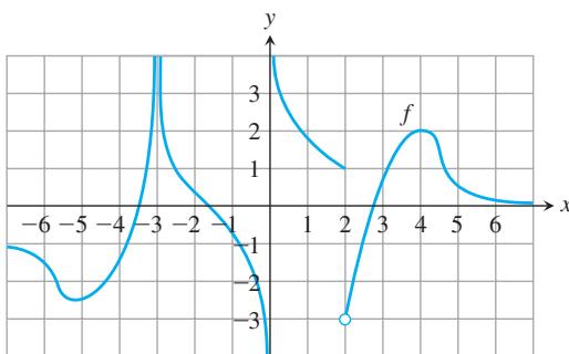
- For the function
𝑓 ∞ − ∞
a.
c.
e.
b.
i.
d.
f.
h.
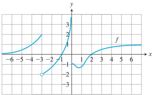
- For the function
𝑓 ∞ − ∞ l i m 𝑥 → 4 𝑓 ( 𝑥 ) l i m 𝑥 → 2 + 𝑓 ( 𝑥 ) l i m 𝑥 → 2 − 𝑓 ( 𝑥 ) l i m 𝑥 → 2 𝑓 ( 𝑥 ) l i m 𝑥 → − 3 + 𝑓 ( 𝑥 ) l i m 𝑥 → − 3 − 𝑓 ( 𝑥 ) l i m 𝑥 → − 3 𝑓 ( 𝑥 ) l i m 𝑥 → 0 + 𝑓 ( 𝑥 ) l i m 𝑥 → 0 − 𝑓 ( 𝑥 )
j.
In Exercises 3–8, find the limit of each function (a) as
-
𝑓 ( 𝑥 ) = 2 𝑥 − 3 -
𝑓 ( 𝑥 ) = 𝜋 − 2 𝑥 2 -
𝑔 ( 𝑥 ) = 1 2 + ( 1 / 𝑥 ) -
𝑔 ( 𝑥 ) = 1 8 − ( 5 / 𝑥 2 ) -
ℎ ( 𝑥 ) = − 5 + ( 7 / 𝑥 ) 3 − ( 1 / 𝑥 2 ) -
ℎ ( 𝑥 ) = 3 − ( 2 / 𝑥 ) 4 + ( √ 2 / 𝑥 2 )
Find the limits in Exercises 9–12.
9.
-
l i m 𝜃 → − ∞ c o s 𝜃 3 𝜃 -
l i m 𝑡 → − ∞ 2 − 𝑡 + s i n 𝑡 𝑡 + c o s 𝑡 -
l i m 𝑟 → ∞ 𝑟 + s i n 𝑟 2 𝑟 + 7 − 5 s i n 𝑟
Limits of Rational Functions
In Exercises 13–22, find the limit of each rational function (a) as
-
𝑓 ( 𝑥 ) = 2 𝑥 + 3 5 𝑥 + 7 -
𝑓 ( 𝑥 ) = 2 𝑥 3 + 7 𝑥 3 − 𝑥 2 + 𝑥 + 7 -
𝑓 ( 𝑥 ) = 𝑥 + 1 𝑥 2 + 3 -
𝑓 ( 𝑥 ) = 3 𝑥 + 7 𝑥 2 − 2 -
ℎ ( 𝑥 ) = 7 𝑥 3 𝑥 3 − 3 𝑥 2 + 6 𝑥 -
ℎ ( 𝑥 ) = 9 𝑥 4 + 𝑥 2 𝑥 4 + 5 𝑥 2 − 𝑥 + 6 -
𝑔 ( 𝑥 ) = 1 0 𝑥 5 + 𝑥 4 + 3 1 𝑥 6 -
𝑔 ( 𝑥 ) = 𝑥 3 + 7 𝑥 2 − 2 𝑥 2 − 𝑥 + 1 -
𝑓 ( 𝑥 ) = 3 𝑥 7 + 5 𝑥 2 − 1 6 𝑥 3 − 7 𝑥 + 3 -
ℎ ( 𝑥 ) = 5 𝑥 8 − 2 𝑥 3 + 9 3 + 𝑥 − 4 𝑥 5
Limits as
The process by which we determine limits of rational functions applies equally well to ratios containing noninteger or negative powers of x.
Divide numerator and denominator by the highest power of x in the denominator and proceed from there. Find the limits in Exercises 23–36. Write
-
l i m 𝑥 → ∞ √ 8 𝑥 2 − 3 2 𝑥 2 + 𝑥 -
l i m 𝑥 → − ∞ ( 𝑥 2 + 𝑥 − 1 8 𝑥 2 − 3 ) 1 / 3 -
l i m 𝑥 → − ∞ ( 1 − 𝑥 3 𝑥 2 + 7 𝑥 ) 5 -
l i m 𝑥 → ∞ √ 𝑥 2 − 5 𝑥 𝑥 3 + 𝑥 − 2 -
l i m 𝑥 → ∞ 2 √ 𝑥 + 𝑥 − 1 3 𝑥 − 7 -
l i m 𝑥 → ∞ 2 + √ 𝑥 2 − √ 𝑥 -
l i m 𝑥 → − ∞ 3 √ 𝑥 − 5 √ 𝑥 3 √ 𝑥 + 5 √ 𝑥 -
l i m 𝑥 → ∞ 𝑥 − 1 + 𝑥 − 4 𝑥 − 2 − 𝑥 − 3 -
l i m 𝑥 → ∞ 2 𝑥 5 / 3 − 𝑥 1 / 3 + 7 𝑥 8 / 5 + 3 𝑥 + √ 𝑥 -
l i m 𝑥 → − ∞ 3 √ 𝑥 − 5 𝑥 + 3 2 𝑥 + 𝑥 2 / 3 − 4 -
l i m 𝑥 → ∞ √ 𝑥 2 + 1 𝑥 + 1 -
l i m 𝑥 → − ∞ √ 𝑥 2 + 1 𝑥 + 1 -
l i m 𝑥 → ∞ 𝑥 − 3 √ 4 𝑥 2 + 2 5 -
l i m 𝑥 → − ∞ 4 − 3 𝑥 3 √ 𝑥 6 + 9
Infinite Limits
Find the limits in Exercises 37–48. Write
-
l i m 𝑥 → 0 + 1 3 𝑥 -
l i m 𝑥 → 0 − 5 2 𝑥 -
l i m 𝑥 → 2 − 3 𝑥 − 2 -
l i m 𝑥 → 3 + 1 𝑥 − 3 -
l i m 𝑥 → − 8 + 2 𝑥 𝑥 + 8 -
l i m 𝑥 → − 5 − 3 𝑥 2 𝑥 + 1 0 -
l i m 𝑥 → 7 4 ( 𝑥 − 7 ) 2 -
l i m 𝑥 → 0 − 1 𝑥 2 ( 𝑥 + 1 ) -
a.
l i m 𝑥 → 0 + 2 3 𝑥 1 / 3 l i m 𝑥 → 0 − 2 3 𝑥 1 / 3 -
a.
l i m 𝑥 → 0 + 2 𝑥 1 / 5 l i m 𝑥 → 0 − 2 𝑥 1 / 5 -
l i m 𝑥 → 0 4 𝑥 2 / 5 -
l i m 𝑥 → 0 1 𝑥 2 / 3
Find the limits in Exercises 49–52. Write
-
l i m 𝑥 → ( 𝜋 / 2 ) − t a n 𝑥 -
l i m 𝑥 → ( − 𝜋 / 2 ) + s e c 𝑥 -
l i m 𝜃 → 0 − ( 1 + c s c 𝜃 ) -
l i m 𝜃 → 0 ( 2 − c o t 𝜃 )
Find the limits in Exercises 53–58. Write
-
l i m 1 𝑥 2 − 4 𝑥 → 2 + 𝑥 → 2 − 𝑥 → − 2 + 𝑥 → − 2 − -
l i m 𝑥 𝑥 2 − 1 𝑥 → 1 + 𝑥 → 1 − 𝑥 → − 1 + 𝑥 → − 1 − -
l i m ( 𝑥 2 2 − 1 𝑥 ) 𝑥 → 0 + 𝑥 → 0 − 𝑥 → 3 √ 2 𝑥 → − 1 -
l i m 𝑥 2 − 1 2 𝑥 + 4 𝑥 → − 2 + 𝑥 → − 2 − 𝑥 → 1 + 𝑥 → 0 − -
l i m 𝑥 2 − 3 𝑥 + 2 𝑥 3 − 2 𝑥 2 𝑥 → 0 + 𝑥 → 2 + 𝑥 → 2 − 𝑥 → 2
e. What, if anything, can be said about the limit as
l i m 𝑥 2 − 3 𝑥 + 2 𝑥 3 − 4 𝑥 𝑥 → 2 + 𝑥 → − 2 + 𝑥 → 0 − 𝑥 → 1 +
e. What, if anything, can be said about the limit as
Find the limits in Exercises 59–62. Write
l i m ( 2 − 3 𝑡 1 / 3 )
a.
b.
l i m ( 1 𝑡 3 / 5 + 7 )
a.
b.
-
l i m ( 1 𝑥 2 / 3 + 2 ( 𝑥 − 1 ) 2 / 3 ) 𝑥 → 0 + 𝑥 → 0 − 𝑥 → 1 + 𝑥 → 1 − -
l i m ( 1 𝑥 1 / 3 − 1 ( 𝑥 − 1 ) 4 / 3 ) 𝑥 → 0 + 𝑥 → 0 − 𝑥 → 1 + 𝑥 → 1 −
Graphing Simple Rational Functions
Graph the rational functions in Exercises 63–68. Include the graphs and equations of the asymptotes and dominant terms.
-
𝑦 = 1 𝑥 − 1 -
𝑦 = 1 𝑥 + 1 -
𝑦 = 1 2 𝑥 + 4 -
𝑦 = − 3 𝑥 − 3 -
𝑦 = 𝑥 + 3 𝑥 + 2 -
𝑦 = 2 𝑥 𝑥 + 1
Domains and Asymptotes
Determine the domain of each function in Exercises 69–74. Then use various limits to find the asymptotes.
-
𝑦 = 4 + 3 𝑥 2 𝑥 2 + 1 -
𝑦 = 2 𝑥 𝑥 2 − 1 -
𝑦 = 8 − 𝑒 𝑥 2 + 𝑒 𝑥 -
𝑦 = 4 𝑒 𝑥 + 𝑒 2 𝑥 𝑒 𝑥 + 𝑒 2 𝑥 -
𝑦 = √ 𝑥 2 + 4 𝑥 -
𝑦 = 𝑥 3 𝑥 3 − 8
Inventing Graphs and Functions
In Exercises 75–78, sketch the graph of a function
-
𝑓 ( 0 ) = 0 , 𝑓 ( 1 ) = 2 , 𝑓 ( − 1 ) = − 2 , l i m 𝑥 → − ∞ 𝑓 ( 𝑥 ) = − 1 , a n d l i m 𝑥 → ∞ 𝑓 ( 𝑥 ) = 1 -
𝑓 ( 0 ) = 0 , l i m 𝑥 → ± ∞ 𝑓 ( 𝑥 ) = 0 , l i m 𝑥 → 0 + 𝑓 ( 𝑥 ) = 2 , a n d l i m 𝑥 → 0 − 𝑓 ( 𝑥 ) = − 2 -
𝑓 ( 0 ) = 0 l i m 𝑥 → ± ∞ 𝑓 ( 𝑥 ) = 0 l i m 𝑥 → 1 − 𝑓 ( 𝑥 ) = l i m 𝑥 → − 1 + 𝑓 ( 𝑥 ) = ∞ l i m 𝑥 → 1 + 𝑓 ( 𝑥 ) = − ∞ , l i m 𝑥 → − 1 − 𝑓 ( 𝑥 ) = − ∞ -
𝑓 ( 2 ) = 1 , 𝑓 ( − 1 ) = 0 , l i m 𝑥 → ∞ 𝑓 ( 𝑥 ) = 0 , l i m 𝑥 → 0 + 𝑓 ( 𝑥 ) = ∞ , l i m 𝑥 → 0 − 𝑓 ( 𝑥 ) = − ∞ , a n d l i m 𝑥 → − ∞ 𝑓 ( 𝑥 ) = 1
In Exercises 79–82, find a function that satisfies the given conditions and sketch its graph. (The answers here are not unique. Any function that satisfies the conditions is acceptable. Feel free to use formulas defined in pieces if that will help.)
-
l i m 𝑥 → ± ∞ 𝑓 ( 𝑥 ) = 0 , l i m 𝑥 → 2 − 𝑓 ( 𝑥 ) = ∞ l i m 𝑥 → 2 + 𝑓 ( 𝑥 ) = ∞ -
l i m 𝑥 → ± ∞ 𝑔 ( 𝑥 ) = 0 , l i m 𝑥 → 3 − 𝑔 ( 𝑥 ) = − ∞ l i m 𝑥 → 3 + 𝑔 ( 𝑥 ) = ∞ -
l i m 𝑥 → − ∞ ℎ ( 𝑥 ) = − 1 , l i m 𝑥 → ∞ ℎ ( 𝑥 ) = 1 , l i m 𝑥 → 0 − ℎ ( 𝑥 ) = − 1 , l i m 𝑥 → 0 + ℎ ( 𝑥 ) = 1 -
l i m 𝑥 → ± ∞ 𝑘 ( 𝑥 ) = 1 , l i m 𝑥 → 1 − 𝑘 ( 𝑥 ) = ∞ , l i m 𝑥 → 1 + 𝑘 ( 𝑥 ) = − ∞ -
Suppose that
𝑓 ( 𝑥 ) 𝑔 ( 𝑥 ) 𝑥 l i m 𝑥 → ∞ ( 𝑓 ( 𝑥 ) / 𝑔 ( 𝑥 ) ) = 2 l i m 𝑥 → − ∞ ( 𝑓 ( 𝑥 ) / 𝑔 ( 𝑥 ) ) -
Suppose that
𝑓 ( 𝑥 ) 𝑔 ( 𝑥 ) 𝑓 ( 𝑥 ) / 𝑔 ( 𝑥 ) 𝑔 ( 𝑥 ) -
How many horizontal asymptotes can the graph of a given rational function have? Give reasons for your answer.
Finding Limits of Differences When 𝑥 → ± ∞
Find the limits in Exercises 86–92. (Hint: Try multiplying and dividing by the conjugate.)
-
l i m 𝑥 → ∞ ( √ 𝑥 + 9 − √ 𝑥 + 4 ) -
l i m 𝑥 → ∞ ( √ 𝑥 2 + 2 5 − √ 𝑥 2 − 1 ) -
l i m 𝑥 → − ∞ ( √ 𝑥 2 + 3 + 𝑥 ) -
l i m 𝑥 → − ∞ ( 2 𝑥 + √ 4 𝑥 2 + 3 𝑥 − 2 ) -
l i m 𝑥 → ∞ ( √ 9 𝑥 2 − 𝑥 − 3 𝑥 ) -
l i m 𝑥 → ∞ ( √ 𝑥 2 + 3 𝑥 − √ 𝑥 2 − 2 𝑥 ) -
l i m 𝑥 → ∞ ( √ 𝑥 2 + 𝑥 − √ 𝑥 2 − 𝑥 )
Using the Formal Definitions
Use the formal definitions of limits as
-
If
𝑓 𝑓 ( 𝑥 ) = 𝑘 l i m 𝑥 → ∞ 𝑓 ( 𝑥 ) = 𝑘 -
If f has the constant value
𝑓 ( 𝑥 ) = 𝑘 l i m 𝑥 → − ∞ 𝑓 ( 𝑥 ) = 𝑘
Use formal definitions to prove the limit statements in Exercises 95–98.
-
l i m 𝑥 → 0 − 1 𝑥 2 = − ∞ -
l i m 𝑥 → 0 1 | 𝑥 | = ∞ -
l i m 𝑥 → 3 − 2 ( 𝑥 − 3 ) 2 = − ∞ -
l i m 𝑥 → − 5 1 ( 𝑥 + 5 ) 2 = ∞ -
Here is the definition of infinite right-hand limit.
Suppose that an interval
if, for every positive real number
Modify the definition to cover the following cases.
a.
b.
c.
Use the formal definitions from Exercise 99 to prove the limit state-
ments in Exercises 100–104.
-
l i m 𝑥 → 0 + 1 𝑥 = ∞ -
l i m 𝑥 → 0 − 1 𝑥 = − ∞
2.6 Continuity
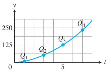
FIGURE 2.56 Connecting plotted points.
l i m 𝑥 → 2 − 1 𝑥 − 2 = − ∞
Continuity at a Point
-
l i m 𝑥 → 2 + 1 𝑥 − 2 = ∞ -
l i m 𝑥 → 1 − 1 1 − 𝑥 2 = ∞
Oblique Asymptotes
Graph the rational functions in Exercises 105–110. Include the graphs and equations of the asymptotes.
-
𝑦 = 𝑥 2 𝑥 − 1 -
𝑦 = 𝑥 2 + 1 𝑥 − 1 -
𝑦 = 𝑥 2 − 4 𝑥 − 1 -
𝑦 = 𝑥 2 − 1 2 𝑥 + 4 -
𝑦 = 𝑥 2 − 1 𝑥 -
𝑦 = 𝑥 3 + 1 𝑥 2
Additional Graphing Exercises
T Graph the curves in Exercises 111–114. Explain the relationship between the curve’s formula and what you see.
-
𝑦 = 𝑥 √ 4 − 𝑥 2 -
𝑦 = − 1 √ 4 − 𝑥 2 -
𝑦 = 𝑥 2 / 3 + 1 𝑥 1 / 3 -
𝑦 = s i n ( 𝜋 𝑥 2 + 1 )
T Graph the functions in Exercises 115 and 116. Then answer the following questions.
a. How does the graph behave as
b. How does the graph behave as
c. How does the graph behave near
Give reasons for your answers.
-
𝑦 = 3 2 ( 𝑥 − 1 𝑥 ) 2 / 3 -
𝑦 = 3 2 ( 𝑥 𝑥 − 1 ) 2 / 3
When we plot function values generated in a laboratory or collected in the field, we often connect the plotted points with an unbroken curve to show what the function’s values are likely to have been at the points we did not measure (Figure 2.56). In doing so, we are assuming that we are working with a continuous function, so its outputs vary regularly and consistently with the inputs, and do not jump abruptly from one value to another without taking on the values in between. Intuitively, any function
To understand continuity, it helps to consider a function like that in Figure 2.57, whose limits we investigated in Example 1 in the last section.
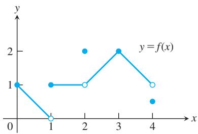
FIGURE 2.57 The function is not continuous at
EXAMPLE 1 At which numbers does the function f in Figure 2.57 appear to be not continuous? Explain why. What occurs at other numbers in the domain?
Solution First we observe that the domain of the function is the closed interval
Numbers at which the graph of f has breaks:
At the interior point x = 1, the function fails to have a limit. It does have both a left-hand limit,
At
At x = 4, the function does have a left-hand limit at this right endpoint,
Numbers at which the graph of 𝑓
At x = 3, the function has a limit,
At
At all other numbers
The following definitions capture the continuity ideas we observed in Example 1.
DEFINITIONS Let c be a real number that is either an interior point or an endpoint of an interval in the domain of f.
The function
is continuous at 𝑓 if 𝑐 l i m 𝑥 → 𝑐 𝑓 ( 𝑥 ) = 𝑓 ( 𝑐 ) . The function f is right-continuous at c (or continuous from the right) if
l i m 𝑥 → 𝑐 + 𝑓 ( 𝑥 ) = 𝑓 ( 𝑐 ) . The function f is left-continuous at c (or continuous from the left) if
l i m 𝑥 → 𝑐 − 𝑓 ( 𝑥 ) = 𝑓 ( 𝑐 ) .
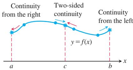
FIGURE 2.58 Continuity at points a, b, and c.
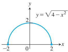
FIGURE 2.59 A function that is continuous over its domain (Example 2).
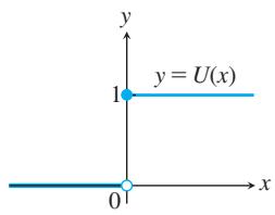
FIGURE 2.60 A function that has a jump discontinuity at the origin (Example 3).
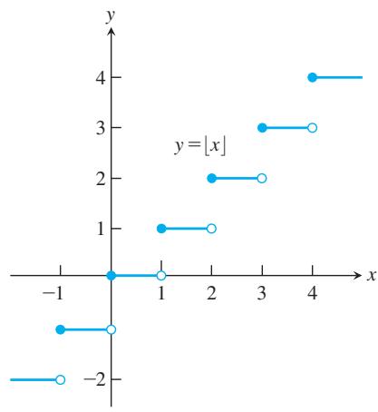
FIGURE 2.61 The greatest integer function is continuous at every noninteger point. It is right-continuous, but not left-continuous, at every integer point (Example 4).
The function f in Example 1 is continuous at every x in [0, 4] except x = 1, 2, and 4. It is right-continuous but not left-continuous at x = 1, neither right- nor left-continuous at x = 2, and not left-continuous at x = 4.
From Theorem 5, it follows immediately that a function f is continuous at an interior point c of an interval in its domain if and only if it is both right-continuous and left-continuous at c (Figure 2.58). We say that a function is continuous over a closed interval
EXAMPLE 2 The function
EXAMPLE 3 The unit step function
At an interior point or an endpoint of an interval in its domain, a function is continuous at points where it passes the following test.
Continuity Test
A function
𝑓 ( 𝑐 ) l i m 𝑥 → 𝑐 𝑓 ( 𝑥 ) 𝑥 → 𝑐 l i m 𝑥 → 𝑐 𝑓 ( 𝑥 ) = 𝑓 ( 𝑐 )
For one-sided continuity, the limits in parts 2 and 3 of the test should be replaced by the appropriate one-sided limits.
EXAMPLE 4 The function
Since
The greatest integer function is continuous at every real number other than the integers. For example,
In general, if
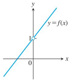
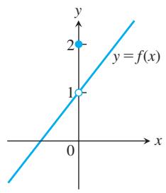
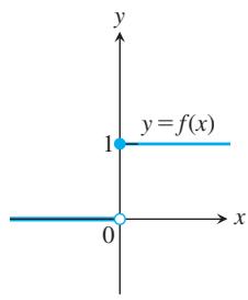
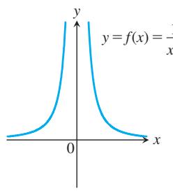
Figure 2.62 displays several common ways in which a function can fail to be continuous. The function in Figure 2.62a is continuous at x = 0. The function in Figure 2.62b does not contain x = 0 in its domain. It would be continuous if its domain were extended so that
FIGURE 2.63 The function
The discontinuities in Figure 2.62d through f are more serious:
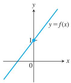
(a)
(b)
(d)
(c)
(e)
(f)
FIGURE 2.62 The function in (a) is continuous at x = 0; the functions in (b) through (f) are not.
Continuous Functions
We now describe the continuity behavior of a function throughout its entire domain, not only at a single point. We define a continuous function to be one that is continuous at every point in its domain. This is a property of the function. A function always has a specified domain, so if we change the domain, then we change the function, and this may change its continuity property as well. If a function is discontinuous at one or more points of its domain, we say it is a discontinuous function.
EXAMPLE 5
(a) The function
(b) The identity function
Algebraic combinations of continuous functions are continuous wherever they are defined.
THEOREM 8—Properties of Continuous Functions If the functions f and g are continuous at x = c, then the following algebraic combinations are continuous at x = c.
- Sums:
𝑓 + 𝑔 𝑓 − 𝑔 𝑘 ⋅ 𝑓 - Products:
𝑓 ⋅ 𝑔 𝑓 / 𝑔 𝑔 ( 𝑐 ) ≠ 0 𝑓 𝑛 - Roots:
𝑛 √ 𝑓
Most of the results in Theorem 8 follow from the limit rules in Theorem 1, Section 2.2. For instance, to prove the sum property we have
This shows that
EXAMPLE 6
(a) Every polynomial
(b) If
EXAMPLE 7 The function
The functions
Inverse Functions and Continuity
When a continuous function defined on an interval has an inverse, the inverse function is itself a continuous function over its own domain. This result is suggested by the observation that the graph of
We defined the exponential function
Continuity of Compositions of Functions
Functions obtained by composing continuous functions are continuous. If
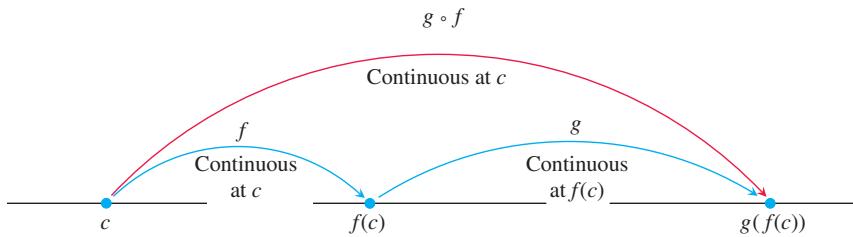
FIGURE 2.64 Compositions of continuous functions are continuous.
THEOREM 9—Compositions of Continuous Functions
If f is continuous at c, and g is continuous at
Intuitively, Theorem 9 is reasonable because if
The continuity of compositions holds for any finite number of compositions of functions. The only requirement is that each function be continuous where it is applied. An outline of a proof of Theorem 9 is given in Exercise 6 in Appendix A.6.
EXAMPLE 8 Show that the following functions are continuous on their natural domains.
(a)
Solution
(a) The square root function is continuous on
(b) The numerator is the cube root of the identity function squared; the denominator is an everywhere-positive polynomial. Therefore, the quotient is continuous.
(c) The quotient
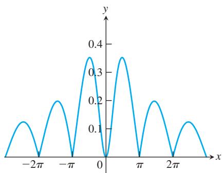
FIGURE 2.65 The graph suggests that
(d) Because the sine function is everywhere-continuous (Exercise 76), the numerator term
Theorem 9 is actually a consequence of a more general result, which we now prove. It states that if the limit of
THEOREM 10—Limits of Continuous Functions
If
Proof Let
Note that if
Since
If we let
which implies from Equation (1) that
EXAMPLE 9 As an application of Theorem 10, we have the following calculations.
Intermediate Value Theorem for Continuous Functions
A function is said to have the Intermediate Value Property if whenever it takes on two values, it also takes on all the values in between.
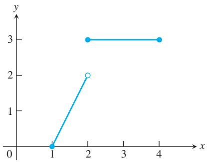
FIGURE 2.66 The function
does not take on all values between
THEOREM 11 - The Intermediate Value Theorem for Continuous Functions If
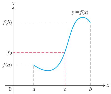
Theorem 11 says that continuous functions over finite closed intervals have the Intermediate Value Property. Geometrically, the Intermediate Value Theorem says that any horizontal line
The proof of the Intermediate Value Theorem depends on the completeness property of the real number system. The completeness property implies that the real numbers have no holes or gaps. In contrast, the rational numbers do not satisfy the completeness property, and a function defined only on the rationals would not satisfy the Intermediate Value Theorem. See Appendix A.9 for a discussion and examples.
The continuity of
A Consequence for Graphing: Connectedness Theorem 11 implies that the graph of a function that is continuous on an interval cannot have any breaks over the interval. It will be connected—a single, unbroken curve. It will not have jumps such as the ones found in the graph of the greatest integer function (Figure 2.61), or separate branches as found in the graph of
A Consequence for Root Finding We call a solution of the equation
In practical terms, when we see the graph of a continuous function cross the horizontal axis on a computer screen, we know it is not stepping across. There really is a point where the function’s value is zero.
EXAMPLE 10 Show that there is a root of the equation
Solution Let
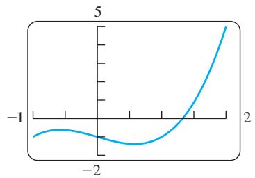
FIGURE 2.68 The curves
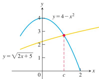
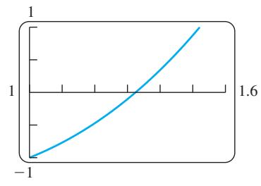
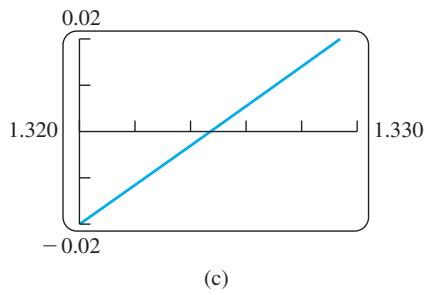
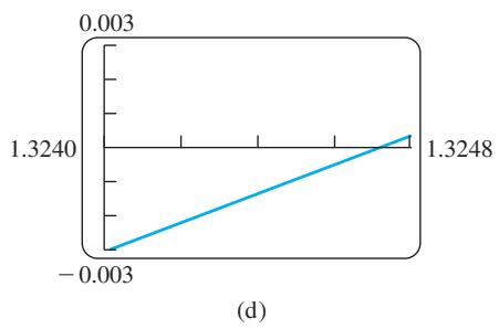
FIGURE 2.67 Zooming in on a zero of the function
EXAMPLE 11 Use the Intermediate Value Theorem to prove that the equation
has a solution (Figure 2.68).
Solution We rewrite the equation as
and set
Continuous Extension to a Point
Sometimes the formula that describes a function
(b)
The new function
so it meets the requirements for continuity (Figure 2.69).
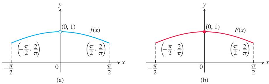
FIGURE 2.69 (a) The graph of
FIGURE 2.70 (a) The graph of
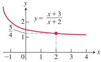
More generally, a function (such as a rational function) may have a limit at a point where it is not defined. If
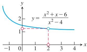
(a)
The function F is continuous at x = c. It is called the continuous extension of f to x = c. For rational functions f, continuous extensions are often found by canceling common factors in the numerator and denominator.
EXAMPLE 12 Show that
has a continuous extension to x = 2, and find that extension.
Solution Although
The new function
is equal to
The graph of f is shown in Figure 2.70. The continuous extension F has the same graph except with no hole at
EXERCISES
Continuity from Graphs
In Exercises 1–4, say whether the function graphed is continuous on
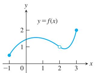
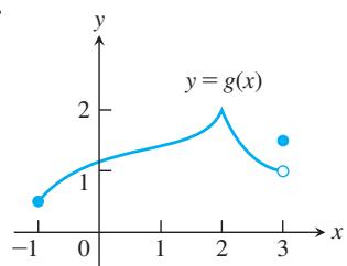
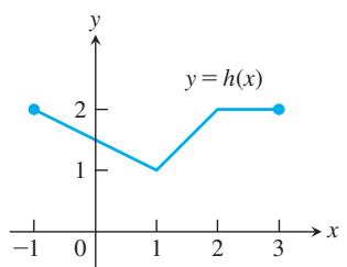
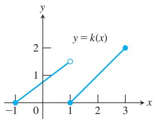
Exercises 5–10 refer to the function
graphed in the accompanying figure.
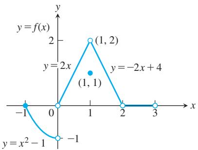
- a. Does
𝑓 ( − 1 )
b. Does
c. Does
d. Is
- a. Does
𝑓 ( 1 )
b. Does
c. Does
d. Is
-
a. Is
𝑓 𝑥 = 2 𝑓 𝑓 𝑥 = 2 -
At what values of
𝑥 𝑓 -
What value should be assigned to
𝑓 ( 2 ) 𝑥 = 2 -
To what new value should
𝑓 ( 1 )
Applying the Continuity Test
At which points do the functions in Exercises 11 and 12 fail to be continuous? At which points, if any, are the discontinuities removable? Not removable? Give reasons for your answers.
-
The function defined in Exercise 1, Section 2.4
-
The function defined in Exercise 2, Section 2.4
At what points are the functions in Exercises 13–32 continuous?
-
𝑦 = 1 𝑥 − 2 − 3 𝑥 -
𝑦 = 1 ( 𝑥 + 2 ) 2 + 4 -
𝑦 = 𝑥 + 1 𝑥 2 − 4 𝑥 + 3 -
𝑦 = 𝑥 + 3 𝑥 2 − 3 𝑥 − 1 0 -
𝑦 = | 𝑥 − 1 | + s i n 𝑥 -
𝑦 = 1 | 𝑥 | + 1 − 𝑥 2 2 -
𝑦 = c o s 𝑥 𝑥 -
𝑦 = 𝑥 + 2 c o s 𝑥 -
𝑦 = c s c 2 𝑥 -
𝑦 = t a n 𝜋 𝑥 2 -
𝑦 = 𝑥 t a n 𝑥 𝑥 2 + 1 -
𝑦 = √ 𝑥 4 + 1 1 + s i n 2 𝑥 -
𝑦 = √ 2 𝑥 + 3 -
𝑦 = 4 √ 3 𝑥 − 1 -
𝑦 = ( 2 𝑥 − 1 ) 1 / 3 -
𝑦 = ( 2 − 𝑥 ) 1 / 5 -
𝑔 ( 𝑥 ) = { 𝑥 2 − 𝑥 − 6 𝑥 − 3 , 𝑥 ≠ 3 5 , 𝑥 = 3 -
𝑓 ( 𝑥 ) = ⎧ { { { ⎨ { { { ⎩ 𝑥 3 − 8 𝑥 2 − 4 , 𝑥 ≠ 2 , 𝑥 ≠ − 2 3 , 𝑥 = 2 4 , 𝑥 = − 2 -
𝑓 ( 𝑥 ) = ⎧ { { ⎨ { { ⎩ 1 − 𝑥 , 𝑥 < 0 𝑒 𝑥 , 0 ≤ 𝑥 ≤ 1 𝑥 2 + 2 , 𝑥 > 1 -
𝑓 ( 𝑥 ) = 𝑥 + 3 2 − 𝑒 𝑥
Limits Involving Trigonometric Functions
Find the limits in Exercises 33–40. Are the functions continuous at the point being approached?
-
l i m 𝑥 → 𝜋 s i n ( 𝑥 − s i n 𝑥 ) -
l i m 𝑡 → 0 s i n ( 𝜋 2 c o s ( t a n 𝑡 ) ) -
l i m 𝑦 → 1 s e c ( 𝑦 s e c 2 𝑦 − t a n 2 𝑦 − 1 ) -
l i m 𝑥 → 0 t a n ( 𝜋 4 c o s ( s i n 𝑥 1 / 3 ) ) -
l i m 𝑡 → 0 c o s ( 𝜋 √ 1 9 − 3 s e c 2 𝑡 ) -
l i m 𝑥 → 𝜋 / 6 √ c s c 2 𝑥 + 5 √ 3 t a n 𝑥 -
l i m 𝑥 → 0 + s i n ( 𝜋 2 𝑒 √ 𝑥 ) -
l i m 𝑥 → 1 c o s − 1 ( l n √ 𝑥 ) -
l i m 𝑥 → 0 s e c [ 𝑒 𝑥 + 𝜋 t a n ( 𝜋 4 s e c 𝑥 ) − 1 ] -
l i m 𝑥 → 0 s i n ( 𝜋 + t a n 𝑥 t a n 𝑥 − 2 s e c 𝑥 ) -
l i m 𝑡 → 0 t a n ( 1 − s i n 𝑡 𝑡 ) -
l i m 𝜃 → 0 c o s ( 𝜋 𝜃 s i n 𝜃 )
Continuous Extensions
-
Define
𝑔 ( 3 ) 𝑔 ( 𝑥 ) = ( 𝑥 2 − 9 ) / ( 𝑥 − 3 ) -
Define
ℎ ( 2 ) ℎ ( 𝑡 ) = ( 𝑡 2 + 3 𝑡 − 1 0 ) / ( 𝑡 − 2 ) -
Define
𝑓 ( 1 ) 𝑓 ( 𝑠 ) = ( 𝑠 3 − 1 ) / ( 𝑠 2 − 1 ) -
Define
𝑔 ( 4 )
to be continuous at x = 4.
- For what value of
𝑎
continuous at every
- For what value of b is
continuous at every
- For what values of
𝑎
continuous at every
- For what values of
𝑏
continuous at every
- For what values of
𝑎 𝑏
continuous at every
- For what values of
𝑎 𝑏
continuous at every
In Exercises 55–58, graph the function f to see whether it appears to have a continuous extension to x = 0. If it does, use Trace and Zoom to find a good candidate for the extended function’s value at x = 0. If the function does not appear to have a continuous extension, can it be extended to be continuous at x = 0 from the right or from the left? If so, what do you think the extended function’s value(s) should be?
𝑓 ( 𝑥 ) = 1 0 𝑥 − 1 𝑥
Theory and Examples
-
A continuous function
𝑦 = 𝑓 ( 𝑥 ) 𝑓 ( 𝑥 ) = 0 -
Explain why the equation
c o s 𝑥 = 𝑥 -
Roots of a cubic Show that the equation
𝑥 3 − 1 5 𝑥 + 1 = 0 [ − 4 , 4 ] -
A function value Show that the function
𝐹 ( 𝑥 ) = ( 𝑥 − 𝑎 ) 2 ( 𝑥 − 𝑏 ) 2 + 𝑥 ( 𝑎 + 𝑏 ) / 2 -
Solving an equation If
𝑓 ( 𝑥 ) = 𝑥 3 − 8 𝑥 + 1 0 𝑓 ( 𝑐 ) 𝜋 − √ 3 -
Explain why the following five statements ask for the same information.
a. Find the roots of
b. Find the x-coordinates of the points where the curve
c. Find all the values of x for which
d. Find the
e. Solve the equation
-
Removable discontinuity Give an example of a function
𝑓 ( 𝑥 ) 𝑥 𝑥 = 2 𝑓 𝑥 = 2 -
Nonremovable discontinuity Give an example of a function
𝑔 ( 𝑥 ) 𝑥 𝑥 = − 1 𝑔 -
A function discontinuous at every point
a. Use the fact that every nonempty interval of real numbers contains both rational and irrational numbers to show that the function
is discontinuous at every point.
b. Is
-
If functions
𝑓 ( 𝑥 ) 𝑔 ( 𝑥 ) 0 ≤ 𝑥 ≤ 1 𝑓 ( 𝑥 ) / 𝑔 ( 𝑥 ) -
If the product function
ℎ ( 𝑥 ) = 𝑓 ( 𝑥 ) ⋅ 𝑔 ( 𝑥 ) 𝑓 ( 𝑥 ) 𝑔 ( 𝑥 ) -
Discontinuous compositions of continuous functions Give an example of functions
𝑓 𝑔 𝑥 = 0 𝑓 ∘ 𝑔 𝑥 = 0 -
Never-zero continuous functions Is it true that a continuous function that is never zero on an interval never changes sign on that interval? Give reasons for your answer.
-
Stretching a rubber band Is it true that if you stretch a rubber band by moving one end to the right and the other to the left, some point of the band will end up in its original position? That is, if x is a position on the rubber band before stretching and
𝑓 ( 𝑥 ) 𝑓 ( 𝑥 ) = 𝑥 -
A fixed point theorem Suppose that a function
𝑓 0 ≤ 𝑓 ( 𝑥 ) ≤ 1 𝑥 𝑐 𝑓 ( 𝑐 ) = 𝑐 𝑐 𝑓 -
The sign-preserving property of continuous functions Let
𝑓 ( 𝑎 , 𝑏 ) 𝑓 ( 𝑐 ) ≠ 0 𝑐 𝑓 ( 𝑐 − 𝛿 , 𝑐 + 𝛿 ) 𝑐 𝑓 𝑓 ( 𝑐 ) -
Prove that
𝑓 𝑐
to prove that both
Solving Equations Graphically
Use the Intermediate Value Theorem in Exercises 77–84 to prove that each equation has a solution. Then use a graphing calculator or computer grapher to solve the equations.
-
𝑥 3 − 3 𝑥 − 1 = 0 7 8 . 2 𝑥 3 − 2 𝑥 2 − 2 𝑥 + 1 = 0 -
𝑥 ( 𝑥 − 1 ) 2 = 1 -
𝑥 𝑥 = 2 -
√ 𝑥 + √ 1 + 𝑥 = 4 -
𝑥 3 − 1 5 𝑥 + 1 = 0 -
c o s 𝑥 = 𝑥 -
2 s i n 𝑥 = 𝑥
CHAPTER 2 Questions to Guide Your Review
-
What is the average rate of change of the function
𝑔 ( 𝑡 ) -
What limit must be calculated to find the rate of change of a function
𝑔 ( 𝑡 ) 𝑡 = 𝑡 0 -
Give an informal or intuitive definition of the limit
Why is the definition “informal”? Give examples.
-
Does the existence and value of the limit of a function
𝑓 ( 𝑥 ) -
What function behaviors might occur for which the limit may fail to exist? Give examples.
-
What theorems are available for calculating limits? Give examples of how the theorems are used.
-
How are one-sided limits related to limits? How can this relationship sometimes be used to calculate a limit or prove it does not exist? Give examples.
-
What is the value of
l i m 𝜃 → 0 ( ( s i n 𝜃 ) / 𝜃 ) 𝜃 -
What exactly does
l i m 𝑥 → 𝑐 𝑓 ( 𝑥 ) = 𝐿 𝛿 > 0 𝑓 , 𝐿 , 𝑐 , 𝜀 > 0 -
Give precise definitions of the following statements.
-
What conditions must be satisfied by a function if it is to be continuous at an interior point of its domain? At an endpoint?
-
How can looking at the graph of a function help you tell where the function is continuous?
-
What does it mean for a function to be right-continuous at a point? Left-continuous? How are continuity and one-sided continuity related?
-
What does it mean for a function to be continuous on an interval? Give examples to illustrate the fact that a function that is not continuous on its entire domain may still be continuous on selected intervals within the domain.
-
What are the basic types of discontinuity? Give an example of each. What is a removable discontinuity? Give an example.
-
What does it mean for a function to have the Intermediate Value Property? What conditions guarantee that a function has this property over an interval? What are the consequences for graphing and solving the equation
𝑓 ( 𝑥 ) = 0 -
Under what circumstances can you extend a function
𝑓 ( 𝑥 ) -
What exactly do
l i m 𝑥 → ∞ 𝑓 ( 𝑥 ) = 𝐿 l i m 𝑥 → − ∞ 𝑓 ( 𝑥 ) = 𝐿 -
What are
l i m 𝑥 → ± ∞ 𝑘 l i m 𝑥 → ± ∞ ( 1 / 𝑥 ) -
How do you find the limit of a rational function as
𝑥 → ± ∞ -
What are horizontal and vertical asymptotes? Give examples.
CHAPTER 2 Practice Exercises
Limits and Continuity
- Graph the function
Then discuss, in detail, limits, one-sided limits, continuity, and one-sided continuity of f at x = -1, 0, and 1. Are any of the discontinuities removable? Explain.
- Repeat the instructions of Exercise 1 for
-
Suppose that
𝑓 ( 𝑡 ) 𝑓 ( 𝑡 ) 𝑡 l i m 𝑡 → 𝑡 0 𝑓 ( 𝑡 ) = − 7 l i m 𝑡 → 𝑡 0 𝑔 ( 𝑡 ) = 0 𝑡 → 𝑡 0 3 𝑓 ( 𝑡 ) ( 𝑓 ( 𝑡 ) ) 2 𝑓 ( 𝑡 ) ⋅ 𝑔 ( 𝑡 ) 𝑓 ( 𝑡 ) 𝑔 ( 𝑡 ) − 7 c o s ( 𝑔 ( 𝑡 ) ) | 𝑓 ( 𝑡 ) | 𝑓 ( 𝑡 ) + 𝑔 ( 𝑡 ) 1 / 𝑓 ( 𝑡 ) -
Suppose the functions
𝑓 ( 𝑥 ) 𝑔 ( 𝑥 ) 𝑥 l i m 𝑥 → 0 𝑓 ( 𝑥 ) = 1 / 2 l i m 𝑥 → 0 𝑔 ( 𝑥 ) = √ 2 𝑥 → 0 − 𝑔 ( 𝑥 ) 𝑔 ( 𝑥 ) ⋅ 𝑓 ( 𝑥 ) 𝑓 ( 𝑥 ) + 𝑔 ( 𝑥 ) 1 / 𝑓 ( 𝑥 ) 𝑥 + 𝑓 ( 𝑥 ) 𝑓 ( 𝑥 ) ⋅ c o s 𝑥 𝑥 − 1
In Exercises 5 and 6, find the value that
-
l i m 𝑥 → 0 ( 4 − 𝑔 ( 𝑥 ) 𝑥 ) = 1 -
l i m 𝑥 → − 4 ( 𝑥 l i m 𝑥 → 0 𝑔 ( 𝑥 ) ) = 2 -
On what intervals are the following functions continuous? a.
𝑓 ( 𝑥 ) = 𝑥 1 / 3 𝑔 ( 𝑥 ) = 𝑥 3 / 4 ℎ ( 𝑥 ) = 𝑥 − 2 / 3 𝑘 ( 𝑥 ) = 𝑥 − 1 / 6 -
On what intervals are the following functions continuous? a.
𝑓 ( 𝑥 ) = t a n 𝑥 𝑔 ( 𝑥 ) = c s c 𝑥 ℎ ( 𝑥 ) = c o s 𝑥 𝑥 − 𝜋 𝑘 ( 𝑥 ) = s i n 𝑥 𝑥
Finding Limits
In Exercises 9–28, find the limit or explain why it does not exist.
-
l i m 𝑥 2 + 𝑥 𝑥 5 + 2 𝑥 4 + 𝑥 3 𝑥 → 0 𝑥 → − 1 -
l i m 𝑥 → 1 1 − √ 𝑥 1 − 𝑥 -
l i m 𝑥 → 𝑎 𝑥 2 − 𝑎 2 𝑥 4 − 𝑎 4 -
l i m ℎ → 0 ( 𝑥 + ℎ ) 2 − 𝑥 2 ℎ -
l i m 𝑥 → 0 ( 𝑥 + ℎ ) 2 − 𝑥 2 ℎ -
l i m 𝑥 → 0 1 2 + 𝑥 − 1 2 𝑥 -
l i m 𝑥 → 0 ( 2 + 𝑥 ) 3 − 8 𝑥 -
l i m 𝑥 → 1 𝑥 1 / 3 − 1 √ 𝑥 − 1 -
l i m 𝑥 → 6 4 𝑥 2 / 3 − 1 6 √ 𝑥 − 8
-
l i m 𝑥 → 𝜋 − c s c 𝑥 -
l i m 𝑥 → 𝜋 s i n ( 𝑥 2 + s i n 𝑥 ) -
l i m 𝑥 → 𝜋 c o s 2 ( 𝑥 − t a n 𝑥 ) -
l i m 𝑥 → 0 8 𝑥 3 s i n 𝑥 − 𝑥 -
l i m 𝑥 → 0 c o s 2 𝑥 − 1 s i n 𝑥 -
l i m 𝑡 → 3 + l n ( 𝑡 − 3 ) -
l i m 𝑡 → 1 𝑡 2 l n ( 2 − √ 𝑡 ) -
l i m 𝜃 → 0 + √ 𝜃 𝑒 c o s ( 𝜋 / 𝜃 ) -
l i m 𝑧 → 0 + 2 𝑒 1 / 𝑧 𝑒 1 / 𝑧 + 1
In Exercises 29–32, find the limit of
-
l i m 𝑥 → 0 + ( 4 𝑔 ( 𝑥 ) ) 1 / 3 = 2 -
l i m 𝑥 → √ 5 1 𝑥 + 𝑔 ( 𝑥 ) = 2 -
l i m 𝑥 → 1 3 𝑥 2 + 1 𝑔 ( 𝑥 ) = ∞ -
l i m 𝑥 → − 2 5 − 𝑥 2 √ 𝑔 ( 𝑥 ) = 0
T Roots
- Let
𝑓 ( 𝑥 ) = 𝑥 3 − 𝑥 − 1
a. Use the Intermediate Value Theorem to show that
b. Solve the equation
c. It can be shown that the exact value of the solution in part (b) is
Evaluate this exact answer and compare it with the value you found in part (b).
T 34. Let
a. Use the Intermediate Value Theorem to show that
b. Solve the equation
c. It can be shown that the exact value of the solution in part (b) is
Evaluate this exact answer and compare it with the value you found in part (b).
Continuous Extension
-
Can
𝑓 ( 𝑥 ) = 𝑥 ( 𝑥 2 − 1 ) / | 𝑥 2 − 1 | 𝑥 = 1 − 1 -
Explain why the function
𝑓 ( 𝑥 ) = s i n ( 1 / 𝑥 )
In Exercises 37–40, graph the function to see whether it appears to have a continuous extension to the given point
-
𝑓 ( 𝑥 ) = 𝑥 − 1 𝑥 − 4 √ 𝑥 , 𝑎 = 1 -
𝑔 ( 𝜃 ) = 5 c o s 𝜃 4 𝜃 − 2 𝜋 , 𝑎 = 𝜋 / 2 -
ℎ ( 𝑡 ) = ( 1 + | 𝑡 | ) 1 / 𝑡 , 𝑎 = 0 -
𝑘 ( 𝑥 ) = 𝑥 1 − 2 | 𝑥 | 𝑎 = 0
Limits at Infinity
Find the limits in Exercises 41–54.
-
l i m 𝑥 → ∞ 2 𝑥 + 3 5 𝑥 + 7 -
l i m 𝑥 → − ∞ 2 𝑥 2 + 3 5 𝑥 2 + 7 -
l i m 𝑥 → − ∞ 𝑥 2 − 4 𝑥 + 8 3 𝑥 3 -
l i m 𝑥 → ∞ 1 𝑥 2 − 7 𝑥 + 1 -
l i m 𝑥 → − ∞ 𝑥 2 − 7 𝑥 𝑥 + 1 -
l i m 𝑥 → ∞ 𝑥 4 + 𝑥 3 1 2 𝑥 3 + 1 2 8 -
l i m 𝑥 → ∞ s i n 𝑥 | 𝑥 | − 5 ≤ 𝑥 ≤ 5 . -
l i m 𝜃 → ∞ c o s 𝜃 − 1 𝜃 𝑓 ( 𝑥 ) = 𝑥 ( c o s ( 1 / 𝑥 ) − 1 ) -
l i m 𝑥 → ∞ 𝑥 + s i n 𝑥 + 2 √ 𝑥 𝑥 + s i n 𝑥 -
l i m 𝑥 → ∞ 𝑥 2 / 3 + 𝑥 − 1 𝑥 2 / 3 + c o s 2 𝑥 -
l i m 𝑥 → ∞ 𝑒 1 / 𝑥 c o s 1 𝑥 -
l i m 𝑡 → ∞ l n ( 1 + 1 𝑡 ) -
l i m 𝑥 → − ∞ t a n − 1 𝑥 -
l i m 𝑡 → − ∞ 𝑒 3 𝑡 s i n − 1 ( 1 𝑡 )
Horizontal and Vertical Asymptotes
-
Use limits to determine the equations for all vertical asymptotes. a.
𝑦 = 𝑥 2 + 4 𝑥 − 3 𝑓 ( 𝑥 ) = 𝑥 2 − 𝑥 − 2 𝑥 2 − 2 𝑥 + 1 𝑦 = 𝑥 2 + 𝑥 − 6 𝑥 2 + 2 𝑥 − 8 -
Use limits to determine the equations for all horizontal asymptotes. a.
𝑦 = 1 − 𝑥 2 𝑥 2 + 1 𝑓 ( 𝑥 ) = √ 𝑥 + 4 √ 𝑥 + 4 𝑔 ( 𝑥 ) = √ 𝑥 2 + 4 𝑥 𝑦 = √ 𝑥 2 + 9 9 𝑥 2 + 1 -
Determine the domain and range of
𝑦 = √ 1 6 − 𝑥 2 𝑥 − 2 -
Assume that constants
𝑎 𝑏 𝑦 = √ 𝑎 𝑥 2 + 4 𝑥 − 𝑏
CHAPTER 2
Additional and Advanced Exercises
T 1. Assigning a value to
If we tried to extend these rules to include the case
We are not dealing with a question of right or wrong here. Neither rule applies as it stands, so there is no contradiction. We could, in fact, define
What value would you like
a. Calculate
b. Graph the function
- A reason you might want
𝟎 0 𝑥 1 / 𝑥 1 / ( l n 𝑥 )
as
a. Evaluate
b. Graph
- Lorentz contraction In relativity theory, the length of an object, say a rocket, appears to an observer to depend on the speed at which the object is traveling with respect to the observer. If the observer measures the rocket’s length as
𝐿 0 𝑣
This equation is the Lorentz contraction formula. Here, c is the speed of light in a vacuum, about
- Controlling the flow from a draining tank Torricelli’s law says that if you drain a tank like the one in the figure shown, the rate
𝑦 𝑥
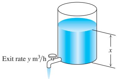
Suppose that
a. within
b. within
- Thermal expansion in precise equipment As you may know, most metals expand when heated and contract when cooled. The dimensions of a piece of laboratory equipment are sometimes so critical that the shop where the equipment is made must be held at the same temperature as the laboratory where the equipment is to be used. A typical aluminum bar that is 10 cm wide at
2 0 ∘
Centimeters wide at a nearby temperature t. Suppose that you are using a bar like this in a gravity wave detector, where its width must stay within 0.0005 cm of the ideal 10 cm. How close to
- Stripes on a measuring cup The interior of a typical 1-L measuring cup is a right circular cylinder of radius 6 cm (see accompanying figure). The volume of water we put in the cup is therefore a function of the level h to which the cup is filled, the formula being
How closely must we measure h to measure out 1 L of water (
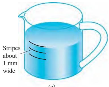
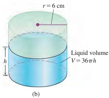
A 1-L measuring cup (a), modeled as a right circular cylinder (b) of radius r = 6 cm
Precise Definition of Limit
In Exercises 7–10, use the formal definition of limit to prove that the function is continuous at c.
-
Uniqueness of limits Show that a function cannot have two different limits at the same point. That is, if
l i m 𝑥 → 𝑐 𝑓 ( 𝑥 ) = 𝐿 1 l i m 𝑥 → 𝑐 𝑓 ( 𝑥 ) = 𝐿 2 𝐿 1 = 𝐿 2 -
Prove the limit Constant Multiple Rule:
l i m 𝑥 → 𝑐 𝑘 𝑓 ( 𝑥 ) = 𝑘 l i m 𝑥 → 𝑐 𝑓 ( 𝑥 ) 𝑘 -
One-sided limits If
l i m 𝑥 → 0 + 𝑓 ( 𝑥 ) = 𝐴 l i m 𝑥 → 0 − 𝑓 ( 𝑥 ) = 𝐵 l i m 𝑥 → 0 + 𝑓 ( 𝑥 3 − 𝑥 ) l i m 𝑥 → 0 − 𝑓 ( 𝑥 3 − 𝑥 ) l i m 𝑥 → 0 + 𝑓 ( 𝑥 2 − 𝑥 4 ) l i m 𝑥 → 0 − 𝑓 ( 𝑥 2 − 𝑥 4 ) -
Limits and continuity Which of the following statements are true, and which are false? If true, say why; if false, give a counterexample (that is, an example confirming the falsehood).
a. If
b. If neither
c. If
d. If
In Exercises 15 and 16, use the formal definition of limit to prove that the function has a continuous extension to the given value of x.
-
𝑓 ( 𝑥 ) = 𝑥 2 − 1 𝑥 + 1 , 𝑥 = − 1 -
𝑔 ( 𝑥 ) = 𝑥 2 − 2 𝑥 − 3 2 𝑥 − 6 , 𝑥 = 3 -
A function continuous at only one point Let
a. Show that
b. Use the fact that every nonempty open interval of real numbers contains both rational and irrational numbers to show that f is not continuous at any nonzero value of x.
- The Dirichlet ruler function If
𝑥 𝑥 𝑚 / 𝑛 𝑛 > 0 𝑚 𝑛 𝑓 ( 𝑥 ) 𝑥
For instance,
a. Show that
b. Show that
c. Sketch the graph of f. Why do you think f is called the “ruler function”?
-
Antipodal points Is there any reason to believe that there is always a pair of antipodal (diametrically opposite) points on Earth’s equator where the temperatures are the same? Explain.
-
If
l i m 𝑥 → 𝑐 ( 𝑓 ( 𝑥 ) + 𝑔 ( 𝑥 ) ) = 3 l i m 𝑥 → 𝑐 ( 𝑓 ( 𝑥 ) − 𝑔 ( 𝑥 ) ) = − 1 l i m 𝑥 → 𝑐 𝑓 ( 𝑥 ) 𝑔 ( 𝑥 ) -
Roots of a quadratic equation that is almost linear The equation
𝑎 𝑥 2 + 2 𝑥 − 1 = 0 𝑎 ≠ 0
a. What happens to
b. What happens to
c. Support your conclusions by graphing
d. For added support, graph
-
Root of an equation Show that the equation
𝑥 + 2 c o s 𝑥 = 0 -
Bounded functions A real-valued function
𝑓 𝐷 𝑁 𝑓 ( 𝑥 ) ≤ 𝑁 𝑥 𝐷 𝑁 𝑓 𝐷 𝑓 𝑁 𝑓 𝐷 𝑀 𝑓 ( 𝑥 ) ≥ 𝑀 𝑥 𝐷 𝑀
a. Show that
b. Suppose that
c. Suppose that
24. Max { 𝑎 , 𝑏 } { 𝑎 , 𝑏 }
a. Show that the expression
equals
b. Find a similar expression for
Generalized Limits Involving
The formula
Here are several examples.
a.
b.
d.
Find the limits in Exercises 25–30.
-
l i m 𝑥 → 0 s i n ( 1 − c o s 𝑥 ) 𝑥 -
l i m 𝑥 → 0 + s i n 𝑥 s i n √ 𝑥 -
l i m 𝑥 → 0 s i n ( s i n 𝑥 ) 𝑥 -
l i m 𝑥 → 0 s i n ( 𝑥 2 + 𝑥 ) 𝑥 -
l i m 𝑥 → 2 s i n ( 𝑥 2 − 4 ) 𝑥 − 2 -
l i m 𝑥 → 9 s i n ( √ 𝑥 − 3 ) 𝑥 − 9
Trigonometric Limits
Find the limits in Exercises 31–38.
-
l i m 𝑥 → 0 s i n 𝑥 2 𝑥 2 − 𝑥 l i m 𝑥 → 0 3 𝑥 − t a n 7 𝑥 2 𝑥 -
l i m 𝑟 → 0 s i n 𝑟 t a n 2 𝑟 l i m 𝜃 → 0 s i n ( s i n 𝜃 ) 𝜃 -
l i m 𝜃 → ( 𝜋 / 2 ) − 4 t a n 2 𝜃 + t a n 𝜃 + 1 t a n 2 𝜃 + 5 -
l i m 𝜃 → 0 + 1 − 2 c o t 2 𝜃 5 c o t 2 𝜃 − 7 c o t 𝜃 − 8 -
l i m 𝑥 → 0 𝑥 s i n 𝑥 2 − 2 c o s 𝑥 -
l i m 𝜃 → 0 1 − c o s 𝜃 𝜃 2
Show how to extend the functions in Exercises 39 and 40 to be continuous at the origin.
-
𝑔 ( 𝑥 ) = t a n ( t a n 𝑥 ) t a n 𝑥 -
𝑓 ( 𝑥 ) = t a n ( t a n 𝑥 ) s i n ( s i n 𝑥 )
Oblique Asymptotes
Find all possible oblique asymptotes in Exercises 41-44.
-
𝑦 = 2 𝑥 3 / 2 + 2 𝑥 − 3 √ 𝑥 + 1 -
𝑦 = 𝑥 + 𝑥 s i n 1 𝑥 -
𝑦 = √ 𝑥 2 + 1 -
𝑦 = √ 𝑥 2 + 2 𝑥
Showing an Equation Is Solvable
- Assume that
1 < 𝑎 < 𝑏 𝑎 𝑥 + 𝑥 = 1 𝑥 − 𝑏 𝑥
More Limits
- Find constants a and b so that each of the following limits is true.
a.
b.
-
Evaluate
l i m 𝑥 → 1 𝑥 2 / 3 − 1 1 − √ 𝑥 -
Evaluate
l i m 𝑥 → 0 | 3 𝑥 + 4 | − | 𝑥 | − 4 𝑥
Limits on Arbitrary Domains
The definition of the limit of a function at x = c extends to functions whose domains near c are more complicated than intervals.
General Definition of Limit
Suppose every open interval containing c contains a point other than c in the domain of f. We say that
For the functions in Exercises 49–52,
a. Find the domain.
b. Show that at
c. Evaluate
-
The function
𝑓 𝑓 ( 𝑥 ) = 𝑥 𝑥 = 1 / 𝑛 𝑛 𝑓 ( 0 ) = 1 -
The function
𝑓 𝑓 ( 𝑥 ) = 1 − 𝑥 𝑥 = 1 / 𝑛 𝑛 𝑓 ( 0 ) = 1 -
𝑓 ( 𝑥 ) = √ 𝑥 s i n ( 1 / 𝑥 ) -
𝑓 ( 𝑥 ) = √ l n ( s i n ( 1 / 𝑥 ) ) -
Let
𝑔 𝑔 ( 𝑥 ) = 2 𝑥 − √ 2 𝑥
a. Sketch the graph of g as well as you can, keeping in mind that g is defined only at rational points.
b. Use the general definition of a limit to prove that
c. Prove that
d. Is
CHAPTER 2 Technology Application Projects
Mathematica/Maple Projects
Projects can be found within MyLab Math.
• Take It to the Limit
Part I
Part II (Zero Raised to the Power Zero: What Does It Mean?)
Part III (One-Sided Limits)
Visualize and interpret the limit concept through graphical and numerical explorations.
Part IV (What a Difference a Power Makes)
See how sensitive limits can be with various powers of x.
- Going to Infinity
Part I (Exploring Function Behavior as
This module provides four examples to explore the behavior of a function as
Part II (Rates of Growth)
Observe graphs that appear to be continuous, yet the function is not continuous. Several issues of continuity are explored to obtain results that you may find surprising.
Derivatives
OVERVIEW In Chapter 2 we discussed how to determine the slope of a curve at a point and how to measure the rate at which a function changes. Now that we have studied limits, we can make these notions precise and see that both are interpretations of the derivative of a function at a point. We then extend this concept from a single point to the derivative function, and we develop rules for finding this derivative function easily, without having to calculate limits directly. These rules are used to find derivatives of most of the common functions reviewed in Chapter 1, as well as combinations of them.