Chapter 14: Multiple Integrals
OVERVIEW In this chapter we define the double integral of a function of two variables
We also define the triple integral of a function of three variables
14.1 Double and Iterated Integrals over Rectangles
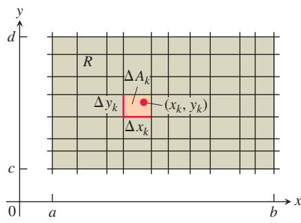
FIGURE 14.1 Rectangular grid partitioning the region R into small rectangles of area
In Chapter 5 we defined the definite integral of a function
Double Integrals
We begin our investigation of double integrals by considering the simplest type of planar region, a rectangle. We consider a function
We subdivide R into small rectangles using a network of lines parallel to the x- and y-axes (Figure 14.1). The lines divide R into n rectangular pieces, where the number of such pieces n gets large as the width and height of each piece gets small. These rectangles form a partition of R. A small rectangular piece of width
FIGURE 14.2 Approximating solids with rectangular boxes leads us to define the volumes of more general solids as double integrals. The volume of the solid shown here is the double integral of
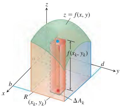
To form a Riemann sum over R, we choose a point
Depending on how we pick
We are interested in what happens to these Riemann sums as the widths and heights of all the small rectangles in the partition of
As
with the understanding that
Many choices are involved in a limit of this kind. The collection of small rectangles is determined by the grid of vertical and horizontal lines that determine a rectangular partition of R. In each of the resulting small rectangles there is a choice of an arbitrary point
When a limit of the sums
It can be shown that if
Double Integrals as Volumes
When
where
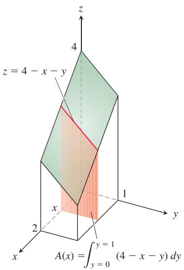
FIGURE 14.4 To obtain the cross-sectional area
As you might expect, this more general method of calculating volume agrees with the methods in Chapter 6, but we do not prove this here. Figure 14.3 shows Riemann sum approximations to the volume becoming more accurate as the number n of boxes increases.
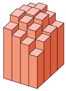
(a) n = 16
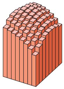
(b) n = 64
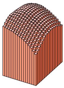
(c) n = 256
FIGURE 14.3 As n increases, the Riemann sum approximations approach the total volume of the solid shown in Figure 14.2.
Fubini’s Theorem for Calculating Double Integrals
Suppose that we wish to calculate the volume under the plane z = 4 - x - y over the rectangular region R:
where
which is the area under the curve z = 4 - x - y in the plane of the cross-section at x. In calculating
We often omit parentheses separating the two integrals in the formula above and write
The expression on the right, called an iterated or repeated integral, says that the volume is obtained by integrating 4 - x - y with respect to y from y = 0 to y = 1 while holding x fixed, and then integrating the resulting expression in x from x = 0 to x = 2. The limits of integration 0 and 1 are associated with y, so they are placed on the integral closest to dy. The other limits of integration, 0 and 2, are associated with the variable x, so they are placed on the outside integral symbol that is paired with dx.
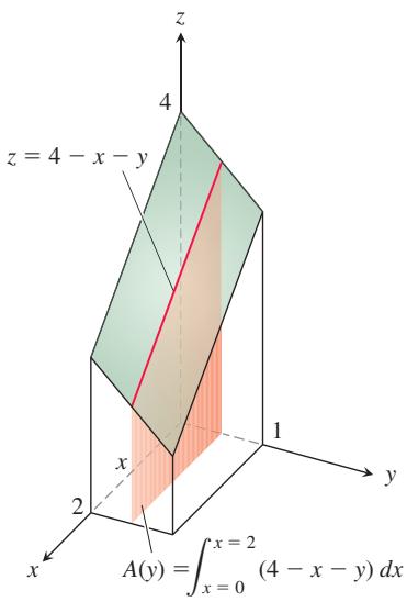
FIGURE 14.5 To obtain the cross-sectional area
HISTORICAL BIOGRAPHY Guido Fubini
(1879–1943)
Fubini attended secondary school in Venice, Italy, where he showed that he was brilliant at mathematics. His advanced study was at the Scuola Normale Superiore di Pisa, where his doctoral thesis was in geometry. He then worked on harmonic functions in curved spaces. Fubini’s interests were wide ranging, from differential geometry to analysis and to the applications of differential equations.
To know more, visit the companion Website.
What would have happened if we had calculated the volume by slicing with planes perpendicular to the y-axis (Figure 14.5)? As a function of y, the typical cross-sectional area is
The volume of the entire solid is therefore
in agreement with our earlier calculation.
Again, we may give a formula for the volume as an iterated integral by writing
The expression on the right says we can find the volume by integrating 4 - x - y with respect to x from x = 0 to x = 2 as in Equation (4) and integrating the result with respect to y from y = 0 to y = 1. In this iterated integral, the order of integration is first x and then y, the reverse of the order in Equation (3).
What do these two volume calculations with iterated integrals have to do with the double integral
over the rectangle
THEOREM 1 – Fubini’s Theorem (First Form)
If
Fubini’s Theorem says that double integrals over rectangles can be calculated as iterated integrals. Thus, we can evaluate a double integral by integrating with respect to one variable at a time using the Fundamental Theorem of Calculus.
Fubini’s Theorem also says that we may calculate the double integral by integrating in either order, a genuine convenience. When we calculate a volume by slicing, we may use either planes perpendicular to the
EXAMPLE 1 Calculate
Reversing the order of integration gives the same answer:
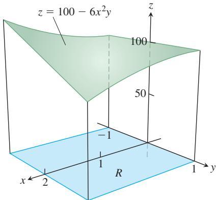
Solution Figure 14.6 displays the volume beneath the surface. By Fubini’s Theorem,
FIGURE 14.6 The double integral
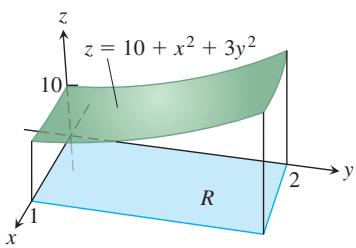
EXAMPLE 2 Find the volume of the region bounded above by the elliptical paraboloid
FIGURE 14.7 The double integral
Solution The surface and volume are shown in Figure 14.7. The volume is given by the double integral
EXERCISES 14.1
Evaluating Iterated Integrals
In Exercises 1–14, evaluate the iterated integral.
-
∫ 2 1 ∫ 4 0 2 𝑥 𝑦 𝑑 𝑦 𝑑 𝑥 -
∫ 2 0 ∫ 1 − 1 ( 𝑥 − 𝑦 ) 𝑑 𝑦 𝑑 𝑥 -
∫ 0 − 1 ∫ 1 − 1 ( 𝑥 + 𝑦 + 1 ) 𝑑 𝑥 𝑑 𝑦 -
∫ 1 0 ∫ 1 0 ( 1 − 𝑥 2 + 𝑦 2 2 ) 𝑑 𝑥 𝑑 𝑦 -
∫ 3 0 ∫ 2 0 ( 4 − 𝑦 2 ) 𝑑 𝑦 𝑑 𝑥 -
∫ 3 0 ∫ 0 − 2 ( 𝑥 2 𝑦 − 2 𝑥 𝑦 ) 𝑑 𝑦 𝑑 𝑥
-
∫ 1 0 ∫ 1 0 𝑦 1 + 𝑥 𝑦 𝑑 𝑥 𝑑 𝑦 -
∫ 4 1 ∫ 4 0 ( 𝑥 2 + √ 𝑦 ) 𝑑 𝑥 𝑑 𝑦 -
∫ l n 2 0 ∫ l n 5 1 𝑒 2 𝑥 + 𝑦 𝑑 𝑦 𝑑 𝑥 -
∫ 1 0 ∫ 2 1 𝑥 𝑦 𝑒 𝑥 𝑑 𝑦 𝑑 𝑥 -
∫ 2 − 1 ∫ 𝜋 / 2 0 𝑦 s i n 𝑥 𝑑 𝑥 𝑑 𝑦 -
∫ 2 𝜋 𝜋 ∫ 𝜋 0 ( s i n 𝑥 + c o s 𝑦 ) 𝑑 𝑥 𝑑 𝑦 -
∫ 4 1 ∫ 𝑒 1 l n 𝑥 𝑥 𝑦 𝑑 𝑥 𝑑 𝑦 -
∫ 2 − 1 ∫ 2 1 𝑥 l n 𝑦 𝑑 𝑦 𝑑 𝑥 -
Find all values of the constant
𝑐 ∫ 1 0 ∫ 𝑐 0 ( 2 𝑥 + 𝑦 ) 𝑑 𝑥 𝑑 𝑦 = 3 -
Find all values of the constant
𝑐
Evaluating Double Integrals over Rectangles
In Exercises 17–24, evaluate the double integral over the given region R.
-
∬ 𝑅 ( 6 𝑦 2 − 2 𝑥 ) 𝑑 𝐴 , 𝑅 : 0 ≤ 𝑥 ≤ 1 , 0 ≤ 𝑦 ≤ 2 -
∬ 𝑅 ( √ 𝑥 𝑦 2 ) 𝑑 𝐴 , 𝑅 : 0 ≤ 𝑥 ≤ 4 , 1 ≤ 𝑦 ≤ 2 -
∬ 𝑅 𝑥 𝑦 c o s 𝑦 𝑑 𝐴 , 𝑅 : − 1 ≤ 𝑥 ≤ 1 , 0 ≤ 𝑦 ≤ 𝜋 -
∬ 𝑅 𝑦 s i n ( 𝑥 + 𝑦 ) 𝑑 𝐴 , 𝑅 : − 𝜋 ≤ 𝑥 ≤ 0 , 0 ≤ 𝑦 ≤ 𝜋 -
∬ 𝑅 𝑒 𝑥 − 𝑦 𝑑 𝐴 , 𝑅 : 0 ≤ 𝑥 ≤ l n 2 , 0 ≤ 𝑦 ≤ l n 2 -
∬ 𝑅 𝑥 𝑦 𝑒 𝑥 𝑦 2 𝑑 𝐴 , 𝑅 : 0 ≤ 𝑥 ≤ 2 , 0 ≤ 𝑦 ≤ 1 -
∬ 𝑅 𝑥 𝑦 3 𝑥 2 + 1 𝑑 𝐴 , 𝑅 : 0 ≤ 𝑥 ≤ 1 , 0 ≤ 𝑦 ≤ 2 -
∬ 𝑅 𝑦 𝑥 2 𝑦 2 + 1 𝑑 𝐴 , 𝑅 : 0 ≤ 𝑥 ≤ 1 , 0 ≤ 𝑦 ≤ 1
In Exercises 25 and 26, integrate f over the given region.
-
Square
𝑓 ( 𝑥 , 𝑦 ) = 1 / ( 𝑥 𝑦 ) 1 ≤ 𝑥 ≤ 2 1 ≤ 𝑦 ≤ 2 -
Rectangle
𝑓 ( 𝑥 , 𝑦 ) = 𝑦 c o s 𝑥 𝑦 0 ≤ 𝑥 ≤ 𝜋 0 ≤ 𝑦 ≤ 1
In Exercises 27 and 28, sketch the solid whose volume is given by the specified integral.
-
∫ 1 0 ∫ 2 0 ( 9 − 𝑥 2 − 𝑦 2 ) 𝑑 𝑦 𝑑 𝑥 -
∫ 3 0 ∫ 4 1 ( 7 − 𝑥 − 𝑦 ) 𝑑 𝑥 𝑑 𝑦 -
Find the volume of the region bounded above by the paraboloid
𝑧 = 𝑥 2 + 𝑦 2 𝑅 − 1 ≤ 𝑥 ≤ 1 − 1 ≤ 𝑦 ≤ 1 -
Find the volume of the region bounded above by the elliptical paraboloid
𝑧 = 1 6 − 𝑥 2 − 𝑦 2 0 ≤ 𝑥 ≤ 2 0 ≤ 𝑦 ≤ 2 -
Find the volume of the region bounded above by the plane
𝑧 = 2 − 𝑥 − 𝑦 𝑅 : 0 ≤ 𝑥 ≤ 1 , 0 ≤ 𝑦 ≤ 1 -
Find the volume of the region bounded above by the plane
𝑧 = 𝑦 / 2 𝑅 : 0 ≤ 𝑥 ≤ 4 , 0 ≤ 𝑦 ≤ 2 -
Find the volume of the region bounded above by the surface
𝑧 = 2 s i n 𝑥 c o s 𝑦 𝑅 : 0 ≤ 𝑥 ≤ 𝜋 / 2 , 0 ≤ 𝑦 ≤ 𝜋 / 4 . -
Find the volume of the region bounded above by the surface
𝑧 = 4 − 𝑦 2 𝑅 : 0 ≤ 𝑥 ≤ 1 , 0 ≤ 𝑦 ≤ 2 -
Find a value of the constant k so that
∫ 2 1 ∫ 3 0 𝑘 𝑥 2 𝑦 𝑑 𝑥 𝑑 𝑦 = 1 -
Evaluate
∫ 1 − 1 ∫ 𝜋 / 2 0 𝑥 s i n √ 𝑦 𝑑 𝑦 𝑑 𝑥 . -
Use Fubini’s Theorem to evaluate
T 39. Use a software application to compute the integrals
Explain why your results do not contradict Fubini’s Theorem.
- If
𝑓 ( 𝑥 , 𝑦 ) 𝑅 𝑎 ≤ 𝑥 ≤ 𝑏 𝑐 ≤ 𝑦 ≤ 𝑑
on the interior of
14.2 Double Integrals over General Regions
| R | |
FIGURE 14.8 A rectangular grid partitioning a bounded, nonrectangular region into rectangular cells.
In this section we define and evaluate double integrals over bounded regions in the plane that are more general than rectangles. These double integrals are also evaluated as iterated integrals, with the main practical problem being that of determining the limits of integration. Since the region of integration may have boundaries other than line segments parallel to the coordinate axes, the limits of integration often involve variables, not just constants.
Double Integrals over Bounded, Nonrectangular Regions
To define the double integral of a function
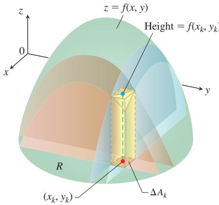
Volume =
FIGURE 14.9 We define the volume of a solid with a curved base as a limit of the sums of volumes of approximating rectangular boxes.
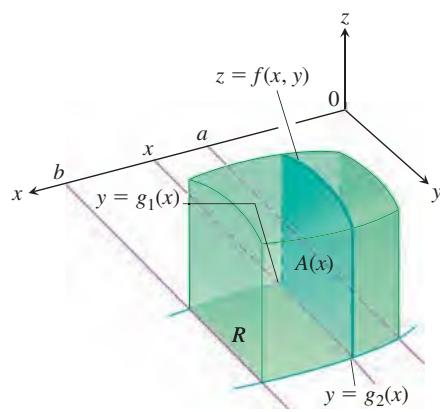
FIGURE 14.10 The area of the vertical slice shown here is
Once we have a partition of R, we number the rectangles in some order from 1 to n and let
As the norm of the partition forming
The nature of the boundary of R introduces issues not found in integrals over an interval. When R has a curved boundary, the n rectangles of a partition lie inside R but do not cover all of R. In order for a partition to approximate R well, the parts of R covered by small rectangles lying partly outside R must become negligible as the norm of the partition approaches zero. This property of being nearly filled in by a partition of small norm is satisfied by all the regions that we will encounter. There is no problem with boundaries made from polygons, circles, and ellipses or from continuous graphs over an interval, joined end to end. A curve with a “fractal” type of shape would be problematic, but such curves arise rarely in most applications. A careful discussion of which types of regions R can be used for computing double integrals is left to a more advanced text.
Volumes
If
If R is a region like the one shown in the xy-plane in Figure 14.10, bounded “above” and “below” by the curves
and then integrate
Similarly, if
That the iterated integrals in Equations (1) and (2) both give the volume that we defined to be the double integral of
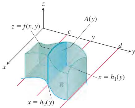
FIGURE 14.11 The volume of the solid shown here is
For a given solid, Theorem 2 says we can calculate the volume as in Figure 14.10 or in the way shown here. Both calculations have the same result.
THEOREM 2—Fubini’s Theorem (Stronger Form)
Let
- If
𝑅 𝑎 ≤ 𝑥 ≤ 𝑏 𝑔 1 ( 𝑥 ) ≤ 𝑦 ≤ 𝑔 2 ( 𝑥 ) 𝑔 1 𝑔 2 [ 𝑎 , 𝑏 ]
- If
𝑅 𝑐 ≤ 𝑦 ≤ 𝑑 ℎ 1 ( 𝑦 ) ≤ 𝑥 ≤ ℎ 2 ( 𝑦 ) ℎ 1 ℎ 2 [ 𝑐 , 𝑑 ]
Some iterated double integrals we will encounter later in this text will use variables of integration other than x and y. For instance, we may write
Regardless of which specific variables of integration are used, the limits of an iterated double integral always satisfy these properties:
-
The limits of the outside integral are constants (they do not depend on either variable of integration), and
-
the limits of the inside integral are functions that may depend on the variable of the outside integral.
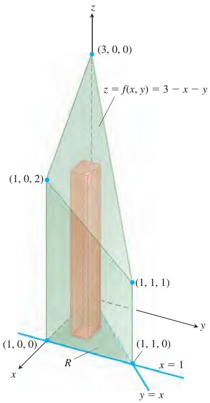
EXAMPLE 1 Find the volume of the right prism whose base is the triangle in the xy-plane bounded by the x-axis and the lines y = x and x = 1 and whose top lies in the plane
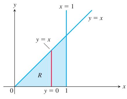
Solution See Figure 14.12a. For any x between 0 and 1, y may vary from y = 0 to y = x (Figure 14.12b). Hence,
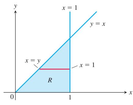
When the order of integration is reversed (Figure 14.12c), the integral for the volume is
The two integrals are equal, as they should be.
Although Fubini’s Theorem assures us that a double integral may be calculated as an iterated integral in either order of integration, the value of one integral may be easier to find than the value of the other. The next example shows how this can happen.
(a)
(b)
(c)
FIGURE 14.12 (a) Prism with a triangular base in the xy-plane. The volume of this prism is defined as a double integral over R. To evaluate it as an iterated integral, we may integrate first with respect to y and then with respect to x, or the other way around (Example 1). (b) Integration limits of
If we integrate first with respect to y, we integrate along a vertical line through R and then integrate from left to right to include all the vertical lines in R. (c) Integration limits of
If we integrate first with respect to x, we integrate along a horizontal line through R and then integrate from bottom to top to include all the horizontal lines in R.
EXAMPLE 2 Calculate
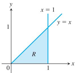
FIGURE 14.13 The region of integration in Example 2.
where R is the triangle in the xy-plane bounded by the x-axis, the line y = x, and the line x = 1.
Solution The region of integration is shown in Figure 14.13. If we integrate first with respect to y and next with respect to x, then because x is held fixed in the first integration, we find
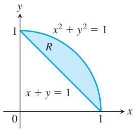
(a)
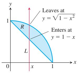
(b)
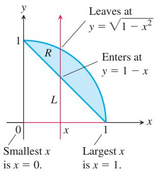
(c)
FIGURE 14.14 Finding the limits of integration when integrating first with respect to y and then with respect to x.
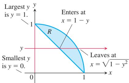
FIGURE 14.15 Finding the limits of integration when integrating first with respect to x and then with respect to y.
If we reverse the order of integration and attempt to calculate
we run into a problem because
There is no general rule for predicting which order of integration will be the good one in circumstances like these. If the order you first choose doesn’t work, try the other. Sometimes neither order will work, and then we may need to use numerical approximations.
Finding Limits of Integration
We now give a procedure for finding limits of integration that applies for many regions in the plane. Regions that are more complicated, and for which this procedure fails, can often be split up into pieces on which the procedure works.
Using Vertical Cross-Sections When faced with evaluating
-
Sketch. Sketch the region of integration and label the bounding curves (Figure 14.14a).
-
Find the y-limits of integration. Imagine a vertical line L cutting through R in the direction of increasing y. Mark the y-values where L enters and leaves. These are the y-limits of integration and are usually functions of x (instead of constants) (Figure 14.14b).
-
Find the x-limits of integration. Choose x-limits that include all the vertical lines through R. These must be constants. The integral whose region of integration is shown in Figure 14.14c is
Using Horizontal Cross-Sections To evaluate the same double integral as an iterated integral with the order of integration reversed, use horizontal lines instead of vertical lines in Steps 2 and 3 (see Figure 14.15). The integral is
EXAMPLE 3 Sketch the region of integration for the integral
and write an equivalent integral with the order of integration reversed.
Solution The region of integration is given by the inequalities
To find limits for integrating in the reverse order, we imagine a horizontal line passing from left to right through the region. It enters at x = y/2 and leaves at
The common value of these integrals is 8.
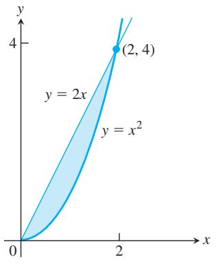
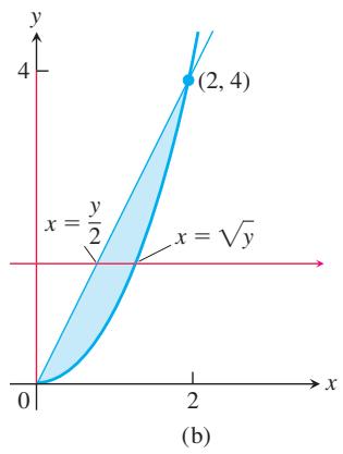
FIGURE 14.16 Region of integration for Example 3.
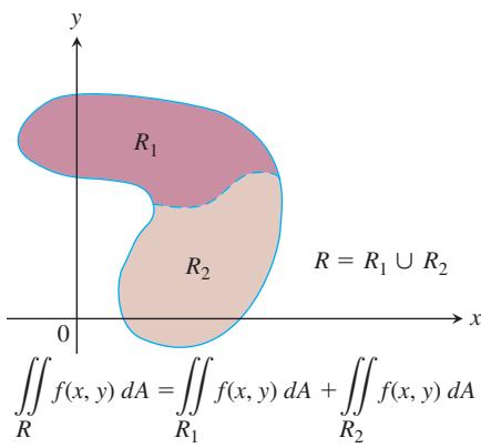
FIGURE 14.17 The Additivity Property for rectangular regions holds for regions bounded by smooth curves.
Properties of Double Integrals
Like single integrals, double integrals of continuous functions have algebraic properties that are useful in computations and applications.
If
-
Constant Multiple:
∬ 𝑅 𝑐 𝑓 ( 𝑥 , 𝑦 ) 𝑑 𝐴 = 𝑐 ∬ 𝑅 𝑓 ( 𝑥 , 𝑦 ) 𝑑 𝐴 𝑐 -
Sum and Difference:
- Domination:
- Additivity: If R is the union of two nonoverlapping regions
𝑅 1 𝑅 2
Property 4 assumes that the region of integration R is decomposed into nonoverlapping regions
The idea behind these properties is that integrals behave like sums. If the function
is replaced by a Riemann sum for cf:
Taking limits as
The other properties are also easy to verify for Riemann sums, and carry over to double integrals for the same reason. While this discussion gives the idea, an actual proof that these properties hold requires a more careful analysis of how Riemann sums converge.
EXAMPLE 4 Find the volume of the wedgelike solid that lies beneath the surface
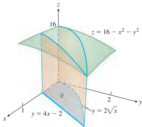
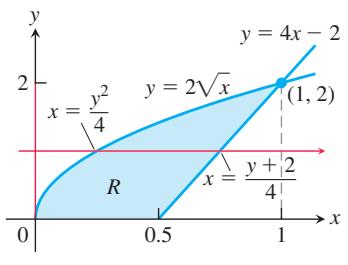
Solution Figure 14.18a shows the surface and the “wedgelike” solid whose volume we want to calculate. Figure 14.18b shows the region of integration in the xy-plane. If we integrate in the order dy dx (first with respect to y and then with respect to x), two integrations will be required because y varies from y = 0 to
(a)
(b)
FIGURE 14.18 (a) The solid “wedge-like” region whose volume is found in Example 4. (b) The region of integration R showing the order dx dy.
Our development of the double integral has focused on its representation of the volume of the solid region between R and the surface
EXERCISES 14.2
Sketching Regions of Integration
In Exercises 1–8, sketch the regions of integration associated with the given double integrals.
-
∫ 3 0 ∫ 2 𝑥 0 𝑓 ( 𝑥 , 𝑦 ) 𝑑 𝑦 𝑑 𝑥 -
∫ 2 − 1 ∫ 𝑥 2 𝑥 − 1 𝑓 ( 𝑥 , 𝑦 ) 𝑑 𝑦 𝑑 𝑥 -
∫ 2 − 2 ∫ 4 𝑦 2 𝑓 ( 𝑥 , 𝑦 ) 𝑑 𝑥 𝑑 𝑦 -
∫ 1 0 ∫ 2 𝑦 𝑦 𝑓 ( 𝑥 , 𝑦 ) 𝑑 𝑥 𝑑 𝑦 -
∫ 1 0 ∫ 𝑒 𝑒 𝑥 𝑓 ( 𝑥 , 𝑦 ) 𝑑 𝑦 𝑑 𝑥 -
∫ 𝑒 2 1 ∫ l n 𝑥 0 𝑓 ( 𝑥 , 𝑦 ) 𝑑 𝑦 𝑑 𝑥 -
∫ 1 0 ∫ a r c s i n 𝑦 0 𝑓 ( 𝑥 , 𝑦 ) 𝑑 𝑥 𝑑 𝑦 -
∫ 8 0 ∫ 𝑦 1 / 3 𝑦 / 4 𝑓 ( 𝑥 , 𝑦 ) 𝑑 𝑥 𝑑 𝑦
Finding Limits of Integration
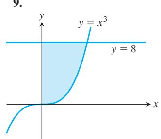
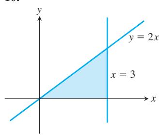
In Exercises 9–18, write an iterated integral for
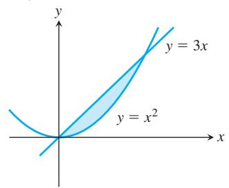
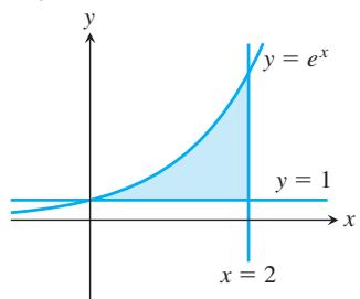
-
Bounded by
𝑦 = √ 𝑥 𝑦 = 0 𝑥 = 9 -
Bounded by
𝑦 = t a n 𝑥 -
Bounded by
𝑦 = 𝑒 − 𝑥 𝑦 = 1 𝑥 = l n 3 -
Bounded by
𝑦 = 0 𝑥 = 0 𝑦 = 1 𝑦 = l n 𝑥 -
Bounded by
𝑦 = 3 − 2 𝑥 𝑦 = 𝑥 𝑥 = 0 -
Bounded by
𝑦 = 𝑥 2 𝑦 = 𝑥 + 2
Evaluating Iterated Integrals
In Exercises 19–26, evaluate the integral.
-
∫ 2 1 ∫ 2 𝑥 0 𝑥 𝑦 3 𝑑 𝑦 𝑑 𝑥 -
∫ 3 1 ∫ 2 𝑦 𝑦 𝑦 𝑑 𝑥 𝑑 𝑦 -
∫ 1 0 ∫ 1 𝑦 ( √ 𝑥 + 𝑥 𝑦 ) 𝑑 𝑥 𝑑 𝑦 -
∫ 2 0 ∫ 𝑥 3 0 ( 𝑦 2 − 𝑥 ) 𝑑 𝑦 𝑑 𝑥 -
∫ √ 𝜋 0 ∫ 𝑥 2 0 𝑥 s i n 𝑦 𝑑 𝑦 𝑑 𝑥 -
∫ 1 0 ∫ a r c t a n 𝑦 0 1 1 + 𝑦 2 𝑑 𝑥 𝑑 𝑦 -
∫ 4 1 ∫ 𝑦 2 𝑦 √ 𝑦 𝑥 𝑑 𝑥 𝑑 𝑦 -
∫ 5 3 ∫ 𝑒 𝑥 1 1 𝑥 𝑦 𝑑 𝑦 𝑑 𝑥
Finding Regions of Integration and Double Integrals
In Exercises 27–32, sketch the region of integration and evaluate the integral.
-
∫ 𝜋 0 ∫ 𝑥 0 𝑥 s i n 𝑦 𝑑 𝑦 𝑑 𝑥 -
∫ 𝜋 0 ∫ s i n 𝑥 0 𝑦 𝑑 𝑦 𝑑 𝑥 -
∫ l n 8 1 ∫ l n 𝑦 1 𝑒 𝑥 + 𝑦 𝑑 𝑥 𝑑 𝑦 -
∫ 2 1 ∫ 𝑦 2 𝑦 𝑑 𝑥 𝑑 𝑦 -
∫ 1 0 ∫ 𝑦 2 0 3 𝑦 3 𝑒 𝑥 𝑦 𝑑 𝑥 𝑑 𝑦 -
∫ 4 1 ∫ √ 𝑥 0 3 2 𝑒 𝑦 / √ 𝑥 𝑑 𝑦 𝑑 𝑥
In Exercises 33–36, integrate f over the given region.
-
Quadrilateral
𝑓 ( 𝑥 , 𝑦 ) = 𝑥 / 𝑦 𝑦 = 𝑥 , 𝑦 = 2 𝑥 , 𝑥 = 1 𝑥 = 2 -
Triangle
𝑓 ( 𝑥 , 𝑦 ) = 𝑥 2 + 𝑦 2 ( 0 , 0 ) , ( 1 , 0 ) ( 0 , 1 ) -
Triangle
𝑓 ( 𝑢 , 𝑣 ) = 𝑣 − √ 𝑢 𝑢 + 𝑣 = 1 -
Curved region
𝑓 ( 𝑠 , 𝑡 ) = 𝑒 𝑠 l n 𝑡 𝑠 = l n 𝑡
Each of Exercises 37–40 gives an integral over a region in a Cartesian coordinate plane. Sketch the region and evaluate the integral.
-
∫ 0 − 2 ∫ − 𝑣 𝑣 2 𝑑 𝑝 𝑑 𝑣 𝑝 𝑣 -
∫ 1 0 ∫ √ 1 − 𝑠 2 0 8 𝑡 𝑑 𝑡 𝑑 𝑠 𝑠 𝑡 -
∫ 𝜋 / 3 − 𝜋 / 3 ∫ s e c 𝑡 0 3 c o s 𝑡 𝑑 𝑢 𝑑 𝑡 𝑡 𝑢 -
∫ 3 / 2 0 ∫ 4 − 2 𝑢 1 4 − 2 𝑢 𝑣 2 𝑑 𝑣 𝑑 𝑢
Reversing the Order of Integration
In Exercises 41–54, sketch the region of integration, and write an equivalent double integral with the order of integration reversed.
-
∫ 1 0 ∫ 4 − 2 𝑥 2 𝑑 𝑦 𝑑 𝑥 -
∫ 2 0 ∫ 0 𝑦 − 2 𝑑 𝑥 𝑑 𝑦 -
∫ 1 0 ∫ √ 𝑦 𝑦 𝑑 𝑥 𝑑 𝑦 -
∫ 1 0 ∫ 1 − 𝑥 2 1 − 𝑥 𝑑 𝑦 𝑑 𝑥 -
∫ 1 0 ∫ 𝑒 𝑥 1 𝑑 𝑦 𝑑 𝑥 -
∫ l n 2 0 ∫ 2 𝑒 𝑦 𝑑 𝑥 𝑑 𝑦 -
∫ 3 / 2 0 ∫ 9 − 4 𝑥 2 0 1 6 𝑥 𝑑 𝑦 𝑑 𝑥 -
∫ 2 0 ∫ 4 − 𝑦 2 0 𝑦 𝑑 𝑥 𝑑 𝑦 -
∫ 1 0 ∫ √ 1 − 𝑦 2 − √ 1 − 𝑦 2 3 𝑦 𝑑 𝑥 𝑑 𝑦 -
∫ 2 0 ∫ √ 4 − 𝑥 2 − √ 4 − 𝑥 2 6 𝑥 𝑑 𝑦 𝑑 𝑥 -
∫ 𝑒 1 ∫ l n 𝑥 0 𝑥 𝑦 𝑑 𝑦 𝑑 𝑥 -
∫ 𝜋 / 6 0 ∫ 1 / 2 s i n 𝑥 𝑥 𝑦 2 𝑑 𝑦 𝑑 𝑥 -
∫ 3 0 ∫ 𝑒 𝑦 1 ( 𝑥 + 𝑦 ) 𝑑 𝑥 𝑑 𝑦 -
∫ √ 3 0 ∫ t a n − 1 𝑦 0 √ 𝑥 𝑦 𝑑 𝑥 𝑑 𝑦
In Exercises 55–64, sketch the region of integration, reverse the order of integration, and evaluate the integral.
-
∫ 𝜋 0 ∫ 𝜋 𝑥 s i n 𝑦 𝑦 𝑑 𝑦 𝑑 𝑥 -
∫ 2 0 ∫ 2 𝑥 2 𝑦 2 s i n 𝑥 𝑦 𝑑 𝑦 𝑑 𝑥 -
∫ 1 0 ∫ 1 𝑦 𝑥 2 𝑒 𝑥 𝑦 𝑑 𝑥 𝑑 𝑦 -
∫ 2 0 ∫ 4 − 𝑥 2 0 𝑥 𝑒 2 𝑦 4 − 𝑦 𝑑 𝑦 𝑑 𝑥 -
∫ 2 √ l n 3 0 ∫ √ l n 3 𝑦 / 2 𝑒 𝑥 2 𝑑 𝑥 𝑑 𝑦 -
∫ 3 0 ∫ 1 √ 𝑥 / 3 𝑒 𝑦 3 𝑑 𝑦 𝑑 𝑥 -
∫ 1 / 1 6 0 ∫ 1 / 2 𝑦 1 / 4 c o s ( 1 6 𝜋 𝑥 5 ) 𝑑 𝑥 𝑑 𝑦 -
∫ 8 0 ∫ 2 3 √ 𝑥 𝑑 𝑦 𝑑 𝑥 𝑦 4 + 1 -
Square region
∬ 𝑅 ( 𝑦 − 2 𝑥 2 ) 𝑑 𝐴 𝑅 | 𝑥 | + | 𝑦 | = 1 -
Triangular region
∬ 𝑅 𝑥 𝑦 𝑑 𝐴 𝑅 𝑦 = 𝑥 𝑦 = 2 𝑥 𝑥 + 𝑦 = 2
Volume Beneath a Surface
-
Find the volume of the region bounded above by the paraboloid
𝑧 = 𝑥 2 + 𝑦 2 𝑥 + 𝑦 = 2 -
Find the volume of the solid that is bounded above by the cylinder
𝑧 = 𝑥 2 𝑦 = 2 − 𝑥 2 -
Find the volume of the solid whose base is the region in the xy-plane that is bounded by the parabola
𝑦 = 4 − 𝑥 2 𝑧 = 𝑥 + 4 -
Find the volume of the solid in the first octant bounded by the coordinate planes, the cylinder
𝑥 2 + 𝑦 2 = 4 𝑧 + 𝑦 = 3 -
Find the volume of the solid in the first octant bounded by the coordinate planes, the plane
𝑥 = 3 𝑧 = 4 − 𝑦 2 -
Find the volume of the solid cut from the first octant by the surface
𝑧 = 4 − 𝑥 2 − 𝑦 -
Find the volume of the wedge cut from the first octant by the cylinder
𝑧 = 1 2 − 3 𝑦 2 𝑥 + 𝑦 = 2 -
Find the volume of the solid cut from the square column
| 𝑥 | + | 𝑦 | ≤ 1 𝑧 = 0 3 𝑥 + 𝑧 = 3 -
Find the volume of the solid that is bounded on the front and back by the planes x = 2 and x = 1, on the sides by the cylinders
𝑦 = ± 1 / 𝑥 𝑧 = 𝑥 + 1 -
Find the volume of the solid bounded on the front and back by the planes
𝑥 = ± 𝜋 / 3 𝑦 = ± s e c 𝑥 𝑧 = 1 + 𝑦 2
In Exercises 75 and 76, sketch the region of integration and the solid whose volume is given by the double integral.
-
∫ 3 0 ∫ 2 − 2 𝑥 / 3 0 ( 1 − 1 3 𝑥 − 1 2 𝑦 ) 𝑑 𝑦 𝑑 𝑥 -
∫ 4 0 ∫ √ 1 6 − 𝑦 2 − √ 1 6 − 𝑦 2 √ 2 5 − 𝑥 2 − 𝑦 2 𝑑 𝑥 𝑑 𝑦
Integrals over Unbounded Regions
Improper double integrals can often be computed similarly to improper integrals of one variable. The first iteration of the following improper integrals is conducted just as if they were proper integrals. One then evaluates an improper integral of a single variable by taking appropriate limits, as in Section 8.8. Evaluate the improper integrals in Exercises 77–80 as iterated integrals.
-
∫ ∞ − ∞ ∫ ∞ − ∞ 1 ( 𝑥 2 + 1 ) ( 𝑦 2 + 1 ) 𝑑 𝑥 𝑑 𝑦 -
∫ ∞ 0 ∫ ∞ 0 𝑥 𝑒 − ( 𝑥 + 2 𝑦 ) 𝑑 𝑥 𝑑 𝑦
Approximating Integrals with Finite Sums
In Exercises 81 and 82, approximate the double integral of
-
𝑓 ( 𝑥 , 𝑦 ) = 𝑥 + 𝑦 𝑦 = √ 1 − 𝑥 2 ( 𝑥 𝑘 , 𝑦 𝑘 ) -
𝑓 ( 𝑥 , 𝑦 ) = 𝑥 + 2 𝑦 ( 𝑥 − 2 ) 2 + ( 𝑦 − 3 ) 2 = 1 ( 𝑥 𝑘 , 𝑦 𝑘 )
Theory and Examples
-
Circular sector Integrate
𝑓 ( 𝑥 , 𝑦 ) = √ 4 − 𝑥 2 𝑥 2 + 𝑦 2 ≤ 4 𝜃 = 𝜋 / 6 𝜃 = 𝜋 / 2 -
Unbounded region Integrate
𝑓 ( 𝑥 , 𝑦 ) = 1 / [ ( 𝑥 2 − 𝑥 ) ( 𝑦 − 1 ) 2 / 3 ] 2 ≤ 𝑥 < ∞ 0 ≤ 𝑦 ≤ 2 -
Noncircular cylinder A solid right (noncircular) cylinder has its base
𝑅 𝑥 𝑦 𝑧 = 𝑥 2 + 𝑦 2
Sketch the base region
- Converting to a double integral Evaluate the integral
(Hint: Write the integrand as an integral.)
- Maximizing a double integral What region
𝑅
Give reasons for your answer.
- Minimizing a double integral What region
𝑅
Give reasons for your answer.
-
Is it possible to evaluate the integral of a continuous function
𝑓 ( 𝑥 , 𝑦 ) 𝑥 𝑦 -
How would you evaluate the double integral of a continuous function
𝑓 ( 𝑥 , 𝑦 ) ( 0 , 1 ) ( 2 , 0 ) ( 1 , 2 ) -
Unbounded region Prove that
COMPUTER EXPLORATIONS
Use a CAS double-integral evaluator to estimate the values of the integrals in Exercises 93–96.
-
∫ 1 0 ∫ 1 0 a r c t a n 𝑥 𝑦 𝑑 𝑦 𝑑 𝑥 -
∫ 1 − 1 ∫ √ 1 − 𝑥 2 0 3 √ 1 − 𝑥 2 − 𝑦 2 𝑑 𝑦 𝑑 𝑥
Use a CAS double-integral evaluator to find the integrals in Exercises 97–102. Then reverse the order of integration and evaluate, again with a CAS.
-
∫ 1 0 ∫ 4 2 𝑦 𝑒 𝑥 2 𝑑 𝑥 𝑑 𝑦 -
∫ 3 0 ∫ 9 𝑥 2 𝑥 c o s ( 𝑦 2 ) 𝑑 𝑦 𝑑 𝑥 -
∫ 2 0 ∫ 4 √ 2 𝑦 𝑦 3 ( 𝑥 2 𝑦 − 𝑥 𝑦 2 ) 𝑑 𝑥 𝑑 𝑦 -
∫ 2 0 ∫ 4 − 𝑦 2 0 𝑒 𝑥 𝑦 𝑑 𝑥 𝑑 𝑦 -
∫ 2 1 ∫ 𝑥 2 0 1 𝑥 + 𝑦 𝑑 𝑦 𝑑 𝑥 -
∫ 2 1 ∫ 8 𝑦 3 1 √ 𝑥 2 + 𝑦 2 𝑑 𝑥 𝑑 𝑦
14.3 Area by Double Integration
In this section we show how to use double integrals to calculate the areas of bounded regions in the plane, and to find the average value of a function of two variables.
Areas of Bounded Regions in the Plane
If we take
This is simply the sum of the areas of the small rectangles in the partition of R, and it approximates what we would like to call the area of R. As the norm of a partition of R approaches zero, the height and width of all rectangles in the partition approach zero, and the coverage of R becomes increasingly complete (Figure 14.8). We define the area of R to be the limit
DEFINITION The area of a closed, bounded plane region R is
𝐴 = ∬ 𝑅 𝑑 𝐴 .
As with the other definitions in this chapter, the definition here applies to a greater variety of regions than does the earlier single-variable definition of area, but it agrees with the earlier definition on regions to which they both apply. To evaluate the integral in the definition of area, we integrate the constant function
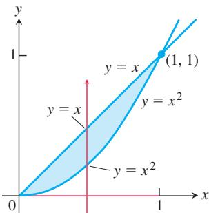
FIGURE 14.19 The region in Example 1.
EXAMPLE 1 Find the area of the region R bounded by y = x and
Solution We sketch the region (Figure 14.19), noting where the two curves intersect at the origin and
Notice that the single-variable integral
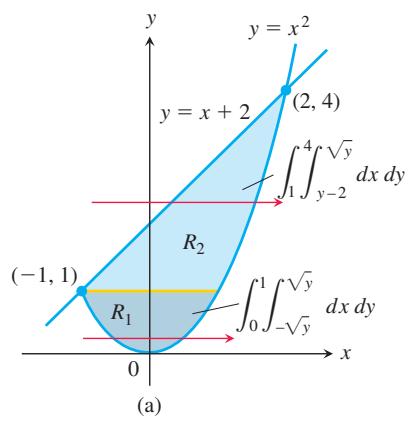
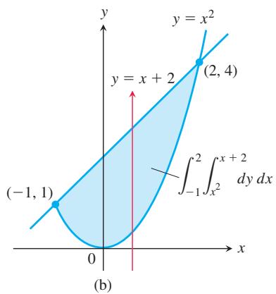
FIGURE 14.20 Calculating this area takes (a) two double integrals if the first integration is with respect to x, but (b) only one if the first integration is with respect to y (Example 2).
EXAMPLE 2 Find the area of the region R enclosed by the parabola
Solution If we divide R into the regions
On the other hand, reversing the order of integration (Figure 14.20b) gives
This second result, which requires only one integral, is simpler to evaluate, giving
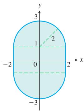
EXAMPLE 3 Find the area of the playing field described by
(a) Fubini’s Theorem
(b) simple geometry.
Solution The region R is shown in Figure 14.21a.
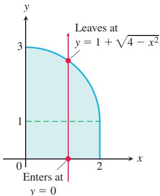
(a) From the symmetries observed in the figure, we see that the area of
Integral Table Formula 45
(b) The region
Average Value
The average value of an integrable function of one variable on a closed interval is the integral of the function over the interval divided by the length of the interval. For an integrable function of two variables defined on a bounded region in the plane, the average value is the integral over the region divided by the area of the region. This can be visualized by thinking of the region as being the base of a tank with vertical walls around the boundary of the region, and imagining that the tank is filled with water that is sloshing around. The value
(a)
(b)
If
EXAMPLE 4 Find the average value of
Solution The value of the integral of f over R is
FIGURE 14.21 (a) The playing field described by the region R in Example 3.
(b) First quadrant of the playing field.
The area of R is
EXERCISES 14.3
Area by Double Integrals
In Exercises 1–12, sketch the region bounded by the given lines and curves. Then express the region’s area as an iterated double integral and evaluate the integral.
-
The coordinate axes and the line
𝑥 + 𝑦 = 2 -
The lines
𝑥 = 0 𝑦 = 2 𝑥 𝑦 = 4 -
The parabola
𝑥 = − 𝑦 2 𝑦 = 𝑥 + 2 -
The parabola
𝑥 = 𝑦 − 𝑦 2 𝑦 = − 𝑥 -
The curve
𝑦 = 𝑒 𝑥 𝑥 = l n 2 -
The curves
𝑦 = l n 𝑥 𝑦 = 2 l n 𝑥 𝑥 = 𝑒 -
The parabolas
𝑥 = 𝑦 2 𝑥 = 2 𝑦 − 𝑦 2 -
𝑥 = 𝑦 2 − 1 a n d 𝑥 = 2 𝑦 2 − 2 -
The lines y = x, y = x/3, and y = 2
-
The lines
𝑦 = 1 − 𝑥 𝑦 = 2 𝑦 = 𝑒 𝑥 -
The lines
𝑦 = 2 𝑥 𝑦 = 𝑥 / 2 𝑦 = 3 − 𝑥 -
The lines
𝑦 = 𝑥 − 2 𝑦 = − 𝑥 𝑦 = √ 𝑥
Identifying the Region of Integration
The integrals and sums of integrals in Exercises 13–18 give the areas of regions in the xy-plane. Sketch each region, label each bounding curve with its equation, and give the coordinates of the points where the curves intersect. Then find the area of the region.
-
∫ 6 0 ∫ 2 𝑦 𝑦 2 / 3 𝑑 𝑥 𝑑 𝑦 -
∫ 3 0 ∫ 𝑥 ( 2 − 𝑥 ) − 𝑥 𝑑 𝑦 𝑑 𝑥 -
∫ 𝜋 / 4 0 ∫ c o s 𝑥 s i n 𝑥 𝑑 𝑦 𝑑 𝑥 -
∫ 2 − 1 ∫ 𝑦 + 2 𝑦 2 𝑑 𝑥 𝑑 𝑦 -
∫ 0 − 1 ∫ 1 − 𝑥 − 2 𝑥 𝑑 𝑦 𝑑 𝑥 + ∫ 2 0 ∫ 1 − 𝑥 − 𝑥 / 2 𝑑 𝑦 𝑑 𝑥 -
∫ 2 0 ∫ 0 𝑥 2 − 4 𝑑 𝑦 𝑑 𝑥 + ∫ 4 0 ∫ √ 𝑥 0 𝑑 𝑦 𝑑 𝑥
Finding Average Values
- Find the average value of
𝑓 ( 𝑥 , 𝑦 ) = s i n ( 𝑥 + 𝑦 )
a. the rectangle
b. the rectangle
-
Which do you think will be larger, the average value of
𝑓 ( 𝑥 , 𝑦 ) = 𝑥 𝑦 0 ≤ 𝑥 ≤ 1 0 ≤ 𝑦 ≤ 1 𝑥 2 + 𝑦 2 ≤ 1 -
Find the average height of the paraboloid
𝑧 = 𝑥 2 + 𝑦 2 0 ≤ 𝑥 ≤ 2 0 ≤ 𝑦 ≤ 2 -
Find the average value of
𝑓 ( 𝑥 , 𝑦 ) = 1 / ( 𝑥 𝑦 ) l n 2 ≤ 𝑥 ≤ 2 l n 2 l n 2 ≤ 𝑦 ≤ 2 l n 2
Theory and Examples
- Geometric area Find the area of the region
using (a) Fubini’s Theorem, (b) simple geometry.
-
Geometric area Find the area of the circular washer with outer radius 2 and inner radius 1, using (a) Fubini’s Theorem, (b) simple geometry.
-
Bacterium population If
𝑓 ( 𝑥 , 𝑦 ) = ( 1 0 , 0 0 0 𝑒 𝑦 ) / ( 1 + | 𝑥 | / 2 ) − 5 ≤ 𝑥 ≤ 5 − 2 ≤ 𝑦 ≤ 0 -
Regional population If
𝑓 ( 𝑥 , 𝑦 ) = 1 0 0 ( 𝑦 + 1 ) 𝑥 = 𝑦 2 𝑥 = 2 𝑦 − 𝑦 2 -
Average temperature in Texas According to the Texas Almanac, Texas has 254 counties and a National Weather Service station in each county. Assume that at time
𝑡 0 𝑡 0 -
If
𝑦 = 𝑓 ( 𝑥 ) 𝑎 ≤ 𝑥 ≤ 𝑏 -
Suppose
𝑓 ( 𝑥 , 𝑦 ) 𝑅 𝐴 ( 𝑅 ) 𝑚 𝑀 𝑚 ≤ 𝑓 ( 𝑥 , 𝑦 ) ≤ 𝑀 ( 𝑥 , 𝑦 ) ∈ 𝑅
- Suppose
𝑓 ( 𝑥 , 𝑦 ) 𝑅 𝐴 ( 𝑅 ) ∬ 𝑅 𝑓 ( 𝑥 , 𝑦 ) 𝑑 𝐴 = 0 𝑓 ( 𝑥 , 𝑦 ) = 0 ( 𝑥 , 𝑦 ) ∈ 𝑅
14.4 Double Integrals in Polar Form
Double integrals are sometimes easier to evaluate if we change to polar coordinates. This section shows how to accomplish the change and how to evaluate double integrals over regions whose boundaries are given by polar equations.
Integrals in Polar Coordinates
When we defined the double integral of a function over a region R in the xy-plane, we began by cutting R into rectangles whose sides were parallel to the coordinate axes. These were the natural shapes to use because their sides have either constant x-values or constant y-values. In polar coordinates, the natural shape is a “polar rectangle” whose sides have constant r- and
Suppose that a function
We cover Q by a grid of circular arcs and rays. The arcs are cut from circles centered at the origin, with radii
where
We number the polar rectangles that lie inside R (the order does not matter), calling their areas
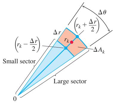
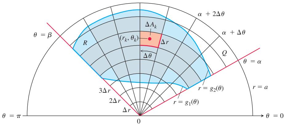
FIGURE 14.23 The observation that
leads to the formula
FIGURE 14.22 The region
If f is continuous throughout R, this sum will approach a limit as we refine the grid to make
To evaluate this limit, we first have to write the sum
The area of a wedge-shaped sector of a circle having radius r and central angle
as can be seen by multiplying
Area of small sector:
Area of large sector:
Therefore,
Combining this result with the sum defining
As
(a)
(b)
(c)
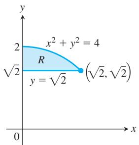
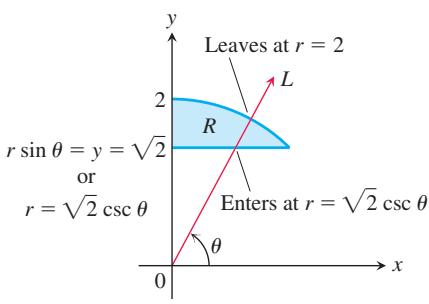
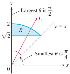
FIGURE 14.24 Finding the limits of integration in polar coordinates.
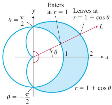
FIGURE 14.25 Finding the limits of integration in polar coordinates for the region in Example 1.
Area Differential in Polar Coordinates
A version of Fubini’s Theorem says that the limit approached by these sums can be evaluated by repeated single integrations with respect to
Finding Limits of Integration
The procedure for finding limits of integration in rectangular coordinates also works for polar coordinates. We illustrate this using the region R shown in Figure 14.24. To evaluate
-
Sketch. Sketch the region and label the bounding curves (Figure 14.24a).
-
Find the r-limits of integration. Imagine a ray L from the origin cutting through R in the direction of increasing r. Mark the r-values where L enters and leaves R. These are the r-limits of integration. They usually depend on the angle
𝜃 -
Find the
𝜃 𝜃 𝜃
EXAMPLE 1 Find the limits of integration for integrating
Solution
-
We first sketch the region and label the bounding curves (Figure 14.25).
-
Next we find the r-limits of integration. A typical ray from the origin enters R where r = 1 and leaves where
𝑟 = 1 + c o s 𝜃 -
Finally, we find the
𝜃 𝑅 𝜃 = − 𝜋 / 2 𝜃 = 𝜋 / 2
If
Area in Polar Coordinates
The area of a closed and bounded region R in the polar coordinate plane is
This formula for area is consistent with all earlier formulas.
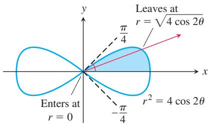
FIGURE 14.26 To integrate over the shaded region, we run r from 0 to
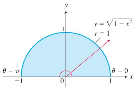
FIGURE 14.27 The semicircular region in Example 3 is the region
EXAMPLE 2 Find the area enclosed by the lemniscate
Solution We graph the lemniscate to determine the limits of integration (Figure 14.26) and see from the symmetry of the region that the total area is 4 times the first-quadrant portion.
Changing Cartesian Integrals into Polar Integrals
The procedure for changing a Cartesian integral
where G denotes the same region of integration, but now described in polar coordinates. This is like the substitution method in Chapter 5 except that there are now two variables to substitute for instead of one. Notice that the area differential dx dy is replaced not by dr dθ but by r dr dθ. A more general discussion of changes of variables (substitutions) in multiple integrals is given in Section 14.8.
EXAMPLE 3 Evaluate
where R is the semicircular region bounded by the x-axis and the curve
Solution In Cartesian coordinates, the integral in question is a nonelementary integral and there is no direct way to integrate
The r in the
EXAMPLE 4 Evaluate the integral
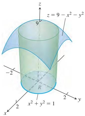
FIGURE 14.28 The solid region in Example 5.
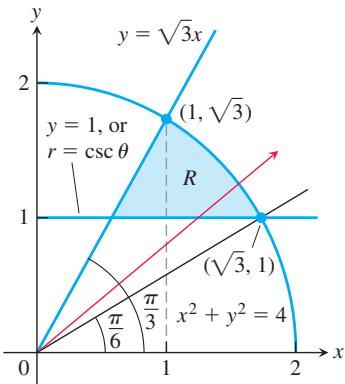
FIGURE 14.29 The region R in Example 6.
Solution Integration with respect to y gives
which is difficult to evaluate without tables. Things go better if we change the original integral to polar coordinates. The region of integration in Cartesian coordinates is given by the inequalities
The polar coordinate transformation is effective here because
EXAMPLE 5 Find the volume of the solid region bounded above by the paraboloid
Solution The region of integration R is bounded by the unit circle
EXAMPLE 6 Using polar integration, find the area of the region R enclosed by the circle
Solution A sketch of the region R is shown in Figure 14.29. First we note that the line
Now, for the region R, as
EXERCISES 14.4
Regions in Polar Coordinates
In Exercises 1–8, describe the given region in polar coordinates.
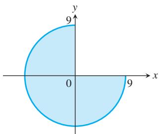
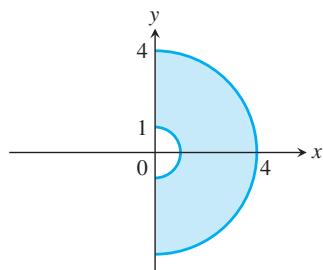
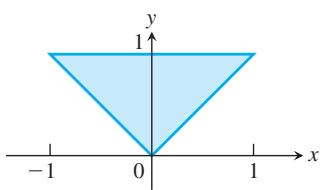
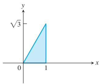
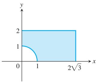
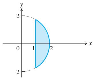
-
The region enclosed by the circle
𝑥 2 + 𝑦 2 = 2 𝑥 -
The region enclosed by the semicircle
𝑥 2 + 𝑦 2 = 2 𝑦 𝑦 ≥ 1
Evaluating Polar Integrals
In Exercises 9–22, change the Cartesian integral into an equivalent polar integral. Then evaluate the polar integral.
-
∫ 1 − 1 ∫ √ 1 − 𝑥 2 0 𝑑 𝑦 𝑑 𝑥 -
∫ 1 0 ∫ √ 1 − 𝑦 2 0 ( 𝑥 2 + 𝑦 2 ) 𝑑 𝑥 𝑑 𝑦 -
∫ 2 0 ∫ √ 4 − 𝑦 2 0 ( 𝑥 2 + 𝑦 2 ) 𝑑 𝑥 𝑑 𝑦 -
∫ 𝑎 − 𝑎 ∫ √ 𝑎 2 − 𝑥 2 − √ 𝑎 2 − 𝑥 2 𝑑 𝑦 𝑑 𝑥 -
∫ 6 0 ∫ 𝑦 0 𝑥 𝑑 𝑥 𝑑 𝑦 -
∫ 2 0 ∫ 𝑥 0 𝑦 𝑑 𝑦 𝑑 𝑥 -
∫ √ 3 1 ∫ 𝑥 1 𝑑 𝑦 𝑑 𝑥 -
∫ 2 √ 2 ∫ 𝑦 √ 4 − 𝑦 2 𝑑 𝑥 𝑑 𝑦 -
∫ 0 − 1 ∫ 0 − √ 1 − 𝑥 2 2 1 + √ 𝑥 2 + 𝑦 2 𝑑 𝑦 𝑑 𝑥 -
∫ 1 − 1 ∫ √ 1 − 𝑥 2 − √ 1 − 𝑥 2 2 ( 1 + 𝑥 2 + 𝑦 2 ) 2 𝑑 𝑦 𝑑 𝑥 -
∫ l n 2 0 ∫ √ ( l n 2 ) 2 − 𝑦 2 0 𝑒 √ 𝑥 2 + 𝑦 2 𝑑 𝑥 𝑑 𝑦 -
∫ 1 − 1 ∫ √ 1 − 𝑦 2 − √ 1 − 𝑦 2 l n ( 𝑥 2 + 𝑦 2 + 1 ) 𝑑 𝑥 𝑑 𝑦 -
∫ 1 0 ∫ √ 2 − 𝑥 2 𝑥 ( 𝑥 + 2 𝑦 ) 𝑑 𝑦 𝑑 𝑥 -
∫ 2 1 ∫ √ 2 𝑥 − 𝑥 2 0 1 ( 𝑥 2 + 𝑦 2 ) 2 𝑑 𝑦 𝑑 𝑥
In Exercises 23–26, sketch the region of integration, and convert each polar integral or sum of integrals into a Cartesian integral or sum of integrals. Do not evaluate the integrals.
-
∫ 𝜋 / 2 0 ∫ 1 0 𝑟 3 s i n 𝜃 c o s 𝜃 𝑑 𝑟 𝑑 𝜃 -
∫ 𝜋 / 2 𝜋 / 6 ∫ c s c 𝜃 1 𝑟 2 c o s 𝜃 𝑑 𝑟 𝑑 𝜃 -
∫ 𝜋 / 4 0 ∫ 2 s e c 𝜃 0 𝑟 5 s i n 2 𝜃 𝑑 𝑟 𝑑 𝜃 -
∫ a r c t a n 4 3 0 ∫ 3 s e c 𝜃 0 𝑟 7 𝑑 𝑟 𝑑 𝜃 + ∫ 𝜋 / 2 a r c t a n 4 3 ∫ 4 c s c 𝜃 0 𝑟 7 𝑑 𝑟 𝑑 𝜃
Area in Polar Coordinates
-
Find the area of the region cut from the first quadrant by the curve
𝑟 = 2 ( 2 − s i n 2 𝜃 ) 1 / 2 -
Cardioid overlapping a circle Find the area of the region that lies inside the cardioid
𝑟 = 1 + c o s 𝜃 -
One leaf of a rose Find the area enclosed by one leaf of the rose
𝑟 = 1 2 c o s 3 𝜃 -
Snail shell Find the area of the region enclosed by the positive x-axis and spiral
𝑟 = 4 𝜃 / 3 0 ≤ 𝜃 ≤ 2 𝜋 -
Cardioid in the first quadrant Find the area of the region cut from the first quadrant by the cardioid
𝑟 = 1 + s i n 𝜃 -
Overlapping cardioids Find the area of the region common to the interiors of the cardioids
𝑟 = 1 + c o s 𝜃 𝑟 = 1 − c o s 𝜃
Average Values
In polar coordinates, the average value of a function over a region R (Section 14.3) is given by
-
Average height of a hemisphere Find the average height of the hemispherical surface
𝑧 = √ 𝑎 2 − 𝑥 2 − 𝑦 2 𝑥 2 + 𝑦 2 ≤ 𝑎 2 -
Average height of a cone Find the average height of the (single) cone
𝑧 = √ 𝑥 2 + 𝑦 2 𝑥 2 + 𝑦 2 ≤ 𝑎 2 -
Average distance from interior of disk to center Find the average distance from a point
𝑃 ( 𝑥 , 𝑦 ) 𝑥 2 + 𝑦 2 ≤ 𝑎 2 -
Average distance squared from a point in a disk to a point in its boundary Find the average value of the square of the distance from the point
𝑃 ( 𝑥 , 𝑦 ) 𝑥 2 + 𝑦 2 ≤ 1 𝐴 ( 1 , 0 )
Theory and Examples
-
Converting to a polar integral Integrate
𝑓 ( 𝑥 , 𝑦 ) = [ l n ( 𝑥 2 + 𝑦 2 ) ] / √ 𝑥 2 + 𝑦 2 1 ≤ 𝑥 2 + 𝑦 2 ≤ 𝑒 -
Converting to a polar integral Integrate
𝑓 ( 𝑥 , 𝑦 ) = [ l n ( 𝑥 2 + 𝑦 2 ) ] / ( 𝑥 2 + 𝑦 2 ) 1 ≤ 𝑥 2 + 𝑦 2 ≤ 𝑒 2 -
Volume of noncircular right cylinder The region that lies inside the cardioid
𝑟 = 1 + c o s 𝜃 𝑟 = 1 𝑧 = 𝑥 -
Volume of noncircular right cylinder The region enclosed by the lemniscate
𝑟 2 = 2 c o s 2 𝜃 𝑧 = √ 2 − 𝑟 2 -
Converting to polar integrals
a. The usual way to evaluate the improper integral
Evaluate the last integral using polar coordinates and solve the resulting equation for I.
b. Evaluate
-
Existence Integrate the function
𝑓 ( 𝑥 , 𝑦 ) = 1 / ( 1 − 𝑥 2 − 𝑦 2 ) 𝑥 2 + 𝑦 2 ≤ 3 / 4 𝑓 ( 𝑥 , 𝑦 ) 𝑥 2 + 𝑦 2 ≤ 1 -
Area formula in polar coordinates Use the double integral in polar coordinates to derive the formula
for the area of the fan-shaped region between the origin and the polar curve
-
Average distance to a given point inside a disk Let
𝑃 0 𝑎 ℎ 𝑃 0 𝑑 𝑃 𝑃 0 𝑑 2 𝑃 0 𝑥 -
Area Suppose that the area of a region in the polar coordinate plane is
Sketch the region and find its area.
-
Evaluate the integral
∬ 𝑅 √ 𝑥 2 + 𝑦 2 𝑑 𝐴 𝑅 𝑥 2 + ( 𝑦 − 1 ) 2 = 1 -
Evaluate the integral
∬ 𝑅 ( 𝑥 2 + 𝑦 2 ) − 2 𝑑 𝐴 𝑅 𝑥 2 + 𝑦 2 = 2 𝑥 ≤ − 1
COMPUTER EXPLORATIONS
In Exercises 49–52, use a CAS to change the Cartesian integrals into an equivalent polar integral and evaluate the polar integral. Perform the following steps in each exercise.
a. Plot the Cartesian region of integration in the xy-plane.
b. Change each boundary curve of the Cartesian region in part (a) to its polar representation by solving its Cartesian equation for r and
c. Using the results in part (b), plot the polar region of integration in the
d. Change the integrand from Cartesian to polar coordinates. Determine the limits of integration from your plot in part (c) and evaluate the polar integral using the CAS integration utility.
-
∫ 1 0 ∫ 1 𝑥 𝑦 𝑥 2 + 𝑦 2 𝑑 𝑦 𝑑 𝑥 5 0 . ∫ 1 0 ∫ 𝑥 / 2 0 𝑥 𝑥 2 + 𝑦 2 𝑑 𝑦 𝑑 𝑥 -
∫ 1 0 ∫ 𝑦 / 3 − 𝑦 / 3 𝑦 √ 𝑥 2 + 𝑦 2 𝑑 𝑥 𝑑 𝑦 -
∫ 1 0 ∫ 2 − 𝑦 𝑦 √ 𝑥 + 𝑦 𝑑 𝑥 𝑑 𝑦
14.5 Triple Integrals in Rectangular Coordinates
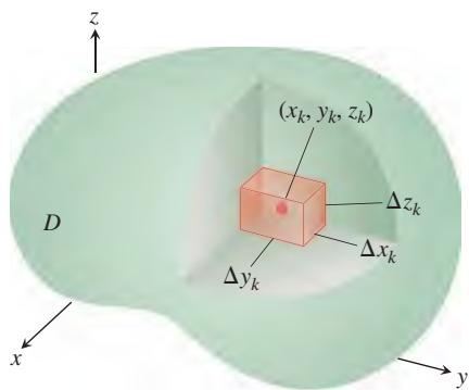
FIGURE 14.30 Partitioning a solid with rectangular cells of volume
Just as double integrals allow us to deal with more general situations than could be handled by single integrals, triple integrals enable us to solve still more general problems. We use triple integrals to calculate the volumes of three-dimensional shapes and the average value of a function over a three-dimensional region. Triple integrals also arise in the study of vector fields and fluid flow in three dimensions, as we will see in Chapter 15.
Triple Integrals
If
We are interested in what happens as D is partitioned by smaller and smaller cells, so that
The regions D over which continuous functions are integrable are those having “reasonably smooth” boundaries.
Volume of a Solid Region in Space
If
As
DEFINITION The volume of a closed and bounded solid region D in space is
𝑉 = ∭ 𝐷 𝑑 𝑉 .
This definition is in agreement with our previous definitions of volume, although we omit the verification of this fact. As we will see in a moment, this integral enables us to calculate the volumes of solids enclosed by curved surfaces. These are more general solids than the ones encountered before (Chapter 6 and Section 14.2).
Iterated Integrals
We evaluate a triple integral by applying a three-dimensional version of Fubini’s Theorem (Section 14.2) to evaluate it by three repeated single integrations. As with double integrals, there is a geometric procedure for finding the limits of integration for these iterated integrals.
To evaluate
over a solid region D, integrate first with respect to z, then with respect to y, and finally with respect to x. (You might choose a different order of integration, but the procedure is similar, as we illustrate in Example 2.)
- Sketch. Sketch the solid region D along with its “shadow” R (vertical projection) in the xy-plane. Label the upper and lower bounding surfaces of D and the upper and lower bounding curves of R.
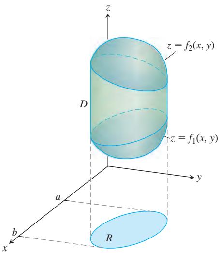
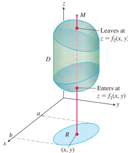
- Find the z-limits of integration. Draw a line M passing through a typical point
( 𝑥 , 𝑦 ) 𝑧 = 𝑓 1 ( 𝑥 , 𝑦 ) 𝑧 = 𝑓 2 ( 𝑥 , 𝑦 )
- Find the y-limits of integration. Draw a line L through
( 𝑥 , 𝑦 ) 𝑦 = 𝑔 1 ( 𝑥 ) 𝑦 = 𝑔 2 ( 𝑥 )
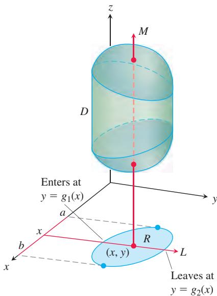
- Find the x-limits of integration. Choose x-limits that include all lines through R parallel to the y-axis (x = a and x = b in the preceding figure). These are the x-limits of integration. The integral is
Follow similar procedures if you change the order of integration. The “shadow” of the solid region D lies in the plane of the last two variables with respect to which the iterated integration takes place. The limits of an iterated triple integral satisfy these properties:
-
The limits of the outside integral are constants (they do not depend on any of the three variables of integration),
-
the limits of the middle integral are functions that may depend on the variable of the outside integral, and
-
the limits of the inside integral are functions that may depend on two variables: the middle integration variable and the outside integration variable.
The preceding procedure applies whenever a solid region D is bounded above and below by a surface, and when the “shadow” region R is bounded by a lower and upper curve. It does not apply to regions with more complicated shapes (such as regions containing holes); although, sometimes such regions can be subdivided into simpler regions for which the procedure does apply.
We illustrate this method of finding the limits of integration in our first example.
EXAMPLE 1 Let S be the sphere of radius 5 centered at the origin, and let D be the solid region under the sphere that lies above the plane z = 3. Set up the limits of integration for evaluating the triple integral of a function
Solution The solid region under the sphere that lies above the plane z = 3 is enclosed by the surfaces
To find the limits of integration, we first sketch the solid region, as shown in Figure 14.31. The “shadow region” R in the xy-plane is a circle of some radius centered at the origin. By considering a side view of the region D, we can determine that the radius of this circle is 4; see Figure 14.32a.
If we fix a point
To find the
Finally, as L sweeps across R from left to right, the value of x varies from x = -4 to x = 4. This gives us the x-limits of integration. Therefore, the triple integral of F over the region D is given by
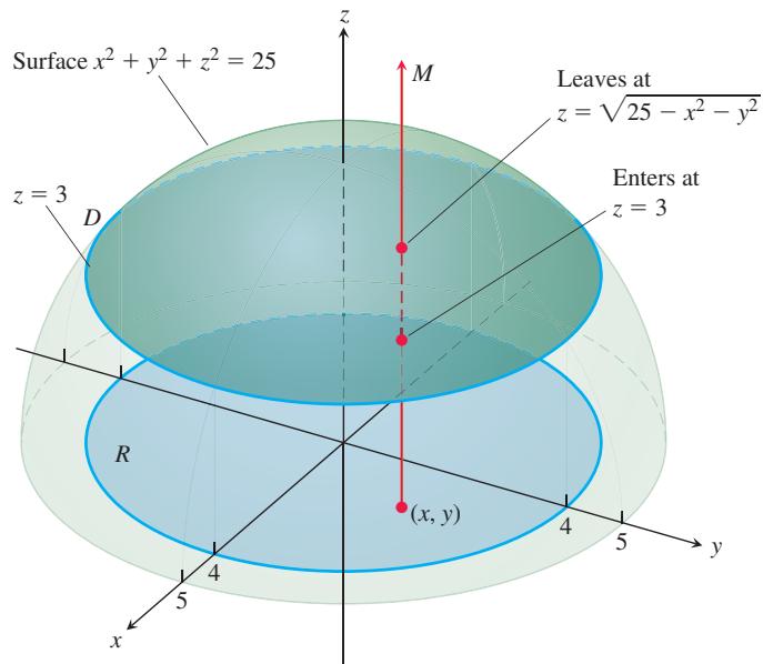
FIGURE 14.31 Finding the limits of integration for evaluating the triple integral of a function defined over the portion of the sphere of radius 5 that lies above the plane z = 3 (Example 1).
(b)
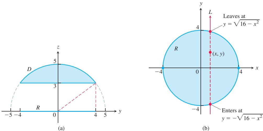
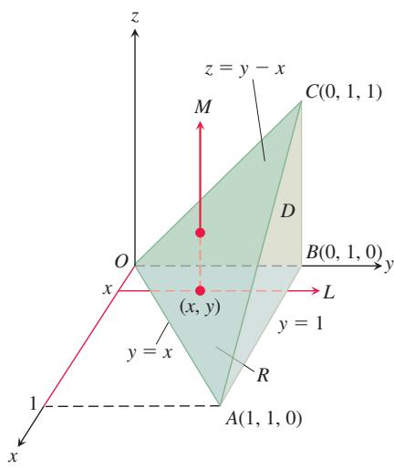
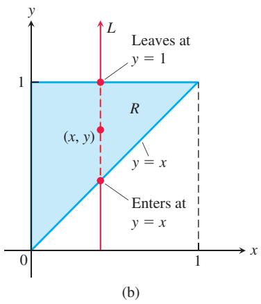
FIGURE 14.33 (a) The tetrahedron in Example 2, showing how the limits of integration are found for the order dz dy dx. (b) The “shadow region” R shown face-on in the xy-plane.
FIGURE 14.32 (a) Side view of the solid region from Example 1, looking down the x-axis. The dashed right triangle has a hypotenuse of length 5 and sides of lengths 3 and 4. In this side view, the shadow region R lies between -4 and 4 on the y-axis. (b) The “shadow region” R shown face-on in the xy-plane.
The region D in Example 1 has a great deal of symmetry, which makes visualization easier. Even without symmetry, the steps in finding the limits of integration are the same, as shown in the next example.
EXAMPLE 2 Set up the limits of integration for evaluating the triple integral of a function
Solution The solid region D and its “shadow” R in the xy-plane are shown in Figure 14.33a. The “top” face is contained in the plane through the points O, A, and C. Following the procedure introduced in Example 7 of Section 11.5, we first form a normal vector to that plane:
and then use this vector and the coordinates of O to set up an equation for the plane:
The “side” face of D is parallel to the xz-plane, the “back” face lies in the yz-plane, and the “bottom” face is contained in the xy-plane.
To find the z-limits of integration, fix a point
To find the y-limits of integration we again fix a point
Finally, as L sweeps across R, the value of x varies from x = 0 to x = 1. Therefore, the triple integral of F over the region D is given by
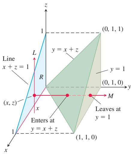
FIGURE 14.34 Finding the limits of integration for evaluating the triple integral of a function defined over the tetrahedron D (Example 3).
In the next example we project the region D onto the xz-plane instead of the xy-plane, to show how to use a different order of integration.
EXAMPLE 3 Find the volume of the tetrahedron D from Example 2 by integrating
Solution Using the limits of integration that we found in Example 2, we calculate the volume of the tetrahedron as follows:
Now we will compute the volume using the order of integration dy dz dx. The procedure for finding the limits of integration is similar, except that we find the limits for y first, then for z, and then for x. The region D is the same tetrahedron as before, but now the “shadow region” R lies in the xz-plane, as shown in Figure 14.34.
To find the y-limits of integration, we fix a point
Next we find the z-limits of integration. The line L that passes through a point
Finally, as
Next we set up and evaluate a triple integral over a more complicated region.
EXAMPLE 4 Find the volume of the solid region D enclosed by the surfaces
Solution The volume is
the integral of
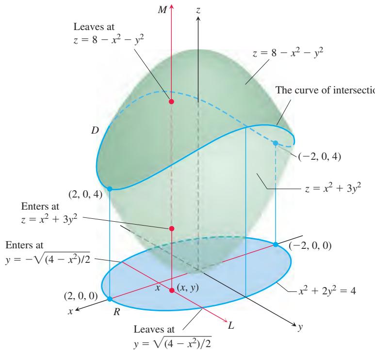
FIGURE 14.35 The volume of the region enclosed by two paraboloids, calculated in Example 4.
Now we find the
Next we find the
Finally, we find the x-limits of integration. As L sweeps across R, the value of x varies from
Average Value of a Function in Space
The average value of a function F over a solid region D in space is defined by the formula
Average value of
For example, if
EXAMPLE 5 Find the average value of
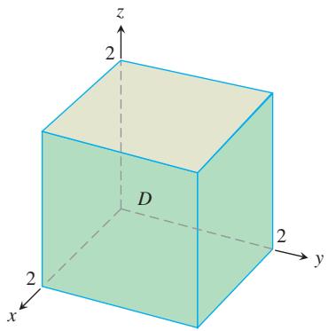
Solution We sketch the cube with enough detail to show the limits of integration (Figure 14.36). We then use Equation (2) to calculate the average value of F over the cube.
FIGURE 14.36 The region of integration in Example 5.
The volume of the region
With these values, Equation (2) gives
In evaluating the integral, we chose the order dx dy dz, but any of the other five possible orders would have done as well.
Properties of Triple Integrals
Triple integrals have the same algebraic properties as double and single integrals. Simply replace the double integrals in the four properties given in Section 14.2, page 864, with triple integrals.
EXERCISES 14.5
Triple Integrals in Different Iteration Orders
-
Evaluate the integral in Example 3, taking
𝐹 ( 𝑥 , 𝑦 , 𝑧 ) = 1 𝑑 𝑧 𝑑 𝑥 𝑑 𝑦 -
Volume of rectangular solid Write six different iterated triple integrals for the volume of the rectangular solid in the first octant bounded by the coordinate planes and the planes x = 1, y = 2, and z = 3. Evaluate one of the integrals.
-
Volume of tetrahedron Write six different iterated triple integrals for the volume of the tetrahedron cut from the first octant by the plane
6 𝑥 + 3 𝑦 + 2 𝑧 = 6 -
Volume of solid Write six different iterated triple integrals for the volume of the solid region in the first octant enclosed by the cylinder
𝑥 2 + 𝑧 2 = 4 -
Volume enclosed by paraboloids Let
𝐷 𝑧 = 8 − 𝑥 2 − 𝑦 2 𝑧 = 𝑥 2 + 𝑦 2 𝐷 -
Volume inside paraboloid beneath a plane Let D be the solid region bounded by the paraboloid
𝑧 = 𝑥 2 + 𝑦 2
Evaluating Triple Iterated Integrals
Evaluate the integrals in Exercises 7–20.
-
∫ 1 0 ∫ 1 0 ∫ 1 0 ( 𝑥 2 + 𝑦 2 + 𝑧 2 ) 𝑑 𝑧 𝑑 𝑦 𝑑 𝑥 -
∫ √ 2 0 ∫ 3 𝑦 0 ∫ 8 − 𝑥 2 − 𝑦 2 𝑥 2 + 3 𝑦 2 𝑑 𝑧 𝑑 𝑥 𝑑 𝑦 -
∫ 𝑒 1 ∫ 𝑒 2 1 ∫ 𝑒 3 1 1 𝑥 𝑦 𝑧 𝑑 𝑥 𝑑 𝑦 𝑑 𝑧 -
∫ 1 0 ∫ 3 − 3 𝑥 0 ∫ 3 − 3 𝑥 − 𝑦 0 𝑑 𝑧 𝑑 𝑦 𝑑 𝑥 -
∫ 𝜋 / 6 0 ∫ 1 0 ∫ 3 − 2 𝑦 s i n 𝑧 𝑑 𝑥 𝑑 𝑦 𝑑 𝑧 -
∫ 1 − 1 ∫ 1 0 ∫ 2 0 ( 𝑥 + 𝑦 + 𝑧 ) 𝑑 𝑦 𝑑 𝑥 𝑑 𝑧 -
∫ 3 0 ∫ √ 9 − 𝑥 2 0 ∫ √ 9 − 𝑥 2 0 𝑑 𝑧 𝑑 𝑦 𝑑 𝑥 -
∫ 2 0 ∫ √ 4 − 𝑦 2 − √ 4 − 𝑦 2 ∫ 2 𝑥 + 𝑦 0 𝑑 𝑧 𝑑 𝑥 𝑑 𝑦 -
∫ 1 0 ∫ 2 − 𝑥 0 ∫ 2 − 𝑥 − 𝑦 0 𝑑 𝑧 𝑑 𝑦 𝑑 𝑥 -
∫ 1 0 ∫ 1 − 𝑥 2 0 ∫ 4 − 𝑥 2 − 𝑦 3 𝑥 𝑑 𝑧 𝑑 𝑦 𝑑 𝑥 -
∫ 𝜋 0 ∫ 𝜋 0 ∫ 𝜋 0 c o s ( 𝑢 + 𝑣 + 𝑤 ) 𝑑 𝑢 𝑑 𝑣 𝑑 𝑤 -
∫ 1 0 ∫ √ 𝑒 1 ∫ 𝑒 1 𝑠 𝑒 𝑠 l n 𝑟 ( l n 𝑡 ) 2 𝑡 𝑑 𝑡 𝑑 𝑟 𝑑 𝑠 -
∫ 𝜋 / 4 0 ∫ l n s e c 𝑣 0 ∫ 2 𝑡 − ∞ 𝑒 𝑥 𝑑 𝑥 𝑑 𝑡 𝑑 𝑣 -
∫ 7 0 ∫ 2 0 ∫ √ 4 − 𝑞 2 0 𝑞 𝑟 + 1 𝑑 𝑝 𝑑 𝑞 𝑑 𝑟
Finding Equivalent Iterated Integrals
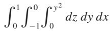
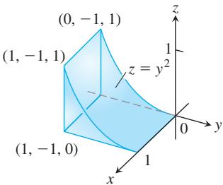
- Here is the region of integration of the integral
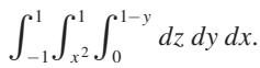
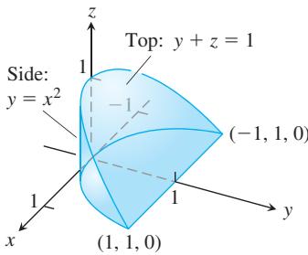
Rewrite the integral as an equivalent iterated integral in the order
a. dy dz dx b. dy dx dz
c.
e. dz dx dy.
- Here is the region of integration of the integral
Rewrite the integral as an equivalent iterated integral in the order
a. dy dz dx b. dy dx dz
c.
e. dz dx dy.
Finding Volumes Using Triple Integrals
Find the volumes of the solid regions in Exercises 23–36.
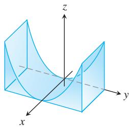
- The region between the cylinder
𝑧 = 𝑦 2 𝑥 𝑦 𝑥 = 0 , 𝑥 = 1 , 𝑦 = − 1 , 𝑦 = 1
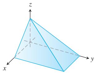
- The region in the first octant bounded by the coordinate planes and the planes
𝑥 + 𝑧 = 1 𝑦 + 2 𝑧 = 2
- The region in the first octant bounded by the coordinate planes, the plane
𝑦 + 𝑧 = 2 𝑥 = 4 − 𝑦 2
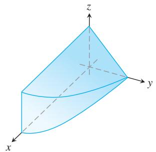
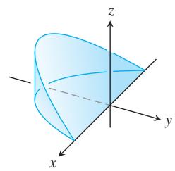
- The wedge cut from the cylinder
𝑥 2 + 𝑦 2 = 1 𝑧 ≥ 0
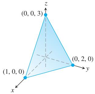
- The tetrahedron in the first octant bounded by the coordinate planes and the plane passing through
( 1 , 0 , 0 ) ( 0 , 2 , 0 ) ( 0 , 0 , 3 )
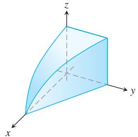
- The region in the first octant bounded by the coordinate planes, the plane
𝑦 = 1 − 𝑥 𝑧 = c o s ( 𝜋 𝑥 / 2 ) 0 ≤ 𝑥 ≤ 1
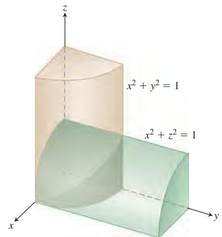
- The region common to the interiors of the cylinders
𝑥 2 + 𝑦 2 = 1 𝑥 2 + 𝑧 2 = 1
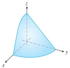
- The region in the first octant bounded by the coordinate planes and the surface
𝑧 = 4 − 𝑥 2 − 𝑦
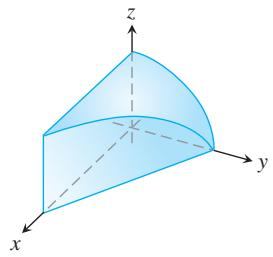
- The region in the first octant bounded by the coordinate planes, the plane
𝑥 + 𝑦 = 4 𝑦 2 + 4 𝑧 2 = 1 6
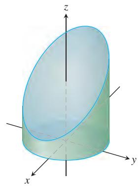
- The region cut from the cylinder
𝑥 2 + 𝑦 2 = 4 𝑥 + 𝑧 = 3
-
The region between the planes
𝑥 + 𝑦 + 2 𝑧 = 2 2 𝑥 + 2 𝑦 + 𝑧 = 4 -
The finite region bounded by the planes
𝑧 = 𝑥 𝑥 + 𝑧 = 8 𝑧 = 𝑦 𝑦 = 8 𝑧 = 0 -
The region cut from the solid elliptical cylinder
𝑥 2 + 4 𝑦 2 ≤ 4 𝑥 𝑦 𝑧 = 𝑥 + 2 -
The region bounded in back by the plane x = 0, on the front and sides by the parabolic cylinder
𝑥 = 1 − 𝑦 2 𝑧 = 𝑥 2 + 𝑦 2
Average Values
In Exercises 37–40, find the average value of
-
𝐹 ( 𝑥 , 𝑦 , 𝑧 ) = 𝑥 2 + 9 -
𝐹 ( 𝑥 , 𝑦 , 𝑧 ) = 𝑥 + 𝑦 − 𝑧 -
𝐹 ( 𝑥 , 𝑦 , 𝑧 ) = 𝑥 2 + 𝑦 2 + 𝑧 2 𝑥 = 1 𝑦 = 1 𝑧 = 1 -
𝐹 ( 𝑥 , 𝑦 , 𝑧 ) = 𝑥 𝑦 𝑧
Changing the Order of Integration
Evaluate the integrals in Exercises 41–44 by changing the order of integration in an appropriate way.
-
∫ 4 0 ∫ 1 0 ∫ 2 2 𝑦 4 c o s ( 𝑥 2 ) 2 √ 𝑧 𝑑 𝑥 𝑑 𝑦 𝑑 𝑧 -
∫ 1 0 ∫ 1 0 ∫ 1 𝑥 2 1 2 𝑥 𝑧 𝑒 𝑧 𝑦 2 𝑑 𝑦 𝑑 𝑥 𝑑 𝑧 -
∫ 1 0 ∫ 1 3 √ 𝑧 ∫ l n 3 0 𝜋 𝑒 2 𝑥 s i n 𝜋 𝑦 2 𝑦 2 𝑑 𝑥 𝑑 𝑦 𝑑 𝑧 -
∫ 2 0 ∫ 4 − 𝑥 2 0 ∫ 𝑥 0 s i n 2 𝑧 4 − 𝑧 𝑑 𝑦 𝑑 𝑧 𝑑 𝑥
Theory and Examples
- Finding an upper limit of an iterated integral Solve for a:
-
Ellipsoid For what value of
𝑐 𝑥 2 + ( 𝑦 / 2 ) 2 + ( 𝑧 / 𝑐 ) 2 = 1 8 𝜋 -
Minimizing a triple integral What domain D in space minimizes the value of the integral
Give reasons for your answer.
- Maximizing a triple integral What domain D in space maximizes the value of the integral
Give reasons for your answer.
COMPUTER EXPLORATIONS
In Exercises 49–52, use a CAS integration utility to evaluate the triple integral of the given function over the specified solid region.
-
𝐹 ( 𝑥 , 𝑦 , 𝑧 ) = 𝑥 2 𝑦 2 𝑧 𝑥 2 + 𝑦 2 = 1 𝑧 = 0 𝑧 = 1 -
𝐹 ( 𝑥 , 𝑦 , 𝑧 ) = | 𝑥 𝑦 𝑧 | 𝑧 = 𝑥 2 + 𝑦 2 -
𝐹 ( 𝑥 , 𝑦 , 𝑧 ) = 𝑧 ( 𝑥 2 + 𝑦 2 + 𝑧 2 ) 3 / 2
by the cone
𝐹 ( 𝑥 , 𝑦 , 𝑧 ) = 𝑥 4 + 𝑦 2 + 𝑧 2 𝑥 2 + 𝑦 2 + 𝑧 2 ≤ 1
14.6 Applications
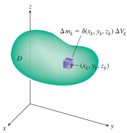
FIGURE 14.37 To define an object’s mass, we first imagine it to be partitioned into a finite number of mass elements
This section shows how to calculate the masses and moments of two- and three-dimensional objects in Cartesian coordinates. The definitions and ideas are similar to the single-variable case we studied in Section 6.6, but now we can consider more general situations.
Masses and First Moments
If
The first moment of a solid region D about a coordinate plane is defined as the triple integral over D of the (signed) distance from a point
The center of mass is found from the first moments. For instance, the
For a two-dimensional object, such as a thin, flat plate, we calculate first moments about the coordinate axes by simply dropping the z-coordinate. So the first moment about the y-axis is the double integral over the region R forming the plate of the (signed) distance from the axis multiplied by the density, or
Table 14.1 summarizes the formulas.
TABLE 14.1 Mass and first moment formulas
THREE-DIMENSIONAL SOLID
Mass:
First moments about the coordinate planes:
Center of mass:
TWO-DIMENSIONAL PLATE
Mass:
First moments:
Center of mass:
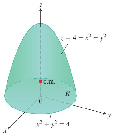
FIGURE 14.38 Finding the center of mass of a solid (Example 1).
EXAMPLE 1 Find the center of mass of a solid of constant density
Solution By symmetry
A similar calculation gives the mass:
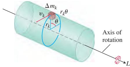
FIGURE 14.40 To find an integral for the amount of energy stored in a rotating shaft, we first imagine the shaft to be partitioned into small blocks. Each block has its own kinetic energy. We add the contributions of the individual blocks to find the kinetic energy of the shaft.
Therefore,
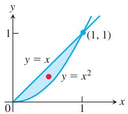
FIGURE 14.39 The centroid of this region is found in Example 2.
When the density of a solid object or plate is constant (as in Example 1), the center of mass is called the centroid of the object. To find a centroid, we set
EXAMPLE 2 Find the centroid of the region in the first quadrant that is bounded above by the line y = x and below by the parabola
Solution We sketch the region and include enough detail to determine the limits of integration (Figure 14.39). We then set
From these values of
The centroid is the point
Note that each coordinate of the centroid of a region is equal to the average value of the corresponding variable over the region.
Moments of Inertia
An object’s first moments (Table 14.1) give us information related to balance and to the torque the object experiences about different axes in a gravitational field. If the object is a rotating shaft, we are interested in how much energy is stored in the shaft and how much energy is generated by a shaft rotating at a particular angular velocity. This is captured by the second moment or moment of inertia.
Think of partitioning the shaft into small blocks of mass
The block’s kinetic energy will be approximately
The kinetic energy of the shaft will be approximately
The integral approached by these sums as the shaft is partitioned into smaller and smaller blocks gives the shaft’s kinetic energy:
The factor
is the moment of inertia of the shaft about its axis of rotation, and we see from Equation (1) that the shaft’s kinetic energy is
The moment of inertia of a shaft resembles in some ways the inertial mass of a locomotive. To start a locomotive with mass m moving at a linear velocity v, we need to provide a kinetic energy of
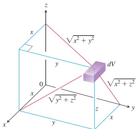
FIGURE 14.41 Distances from dV to the axes.
We now derive a formula for the moment of inertia for a solid in space. If
If L is the x-axis, then
Similarly, if L is the y-axis or the z-axis, we have
Table 14.2 summarizes the formulas for these moments of inertia (second moments because they invoke the squares of the distances). It shows the definition of the polar moment about the origin as well.
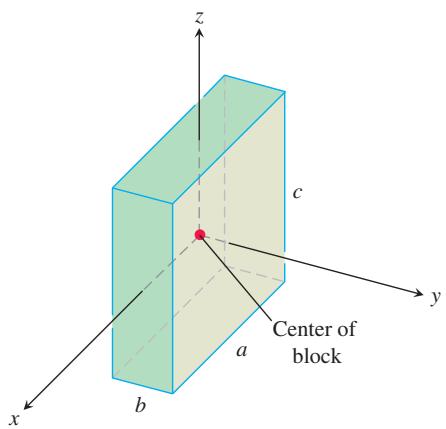
FIGURE 14.42 Finding
TABLE 14.2 Moments of inertia (second moments) formulas
THREE-DIMENSIONAL SOLID
About the x-axis:
EXAMPLE 3 Find
Solution The formula for
We can avoid some of the work of integration by observing that
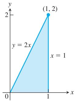
FIGURE 14.43 The triangular region covered by the plate in Example 4.
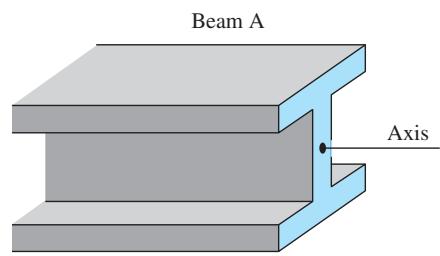
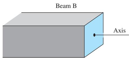
FIGURE 14.44 The greater the polar moment of inertia of the cross-section of a beam about the beam’s longitudinal axis, the stiffer the beam. Beams A and B have the same cross-sectional area, but A is stiffer.
Similarly,
EXAMPLE 4 A thin plate covers the triangular region bounded by the x-axis and the lines x = 1 and y = 2x in the first quadrant. The plate’s density at the point
Solution We sketch the plate and put in enough detail to determine the limits of integration for the integrals we have to evaluate (Figure 14.43). The moment of inertia about the x-axis is
Similarly, the moment of inertia about the y-axis is
Notice that we integrate
The moment of inertia also plays a role in determining how much a horizontal metal beam will bend under a load. The stiffness of the beam is a constant times
Probability
The probability that a continuous random variable X takes values between a and b is found by integrating a probability density function f (Appendix A.8),
A similar process applies to probabilities involving two continuous random variables. The probability that a pair of random variables
If the region is a rectangle, then this expression has the simple form
A joint probability density function f is defined by three basic properties. The first property ensures that there are no negative probabilities, and the second implies that the total probability of all possible outcomes is one. The final property describes the connection of f to probabilities.
DEFINITION A joint probability density function
is a function that satisfies three conditions: 𝑓
𝑓 ( 𝑥 , 𝑦 ) ≥ 0 ∫ ∞ − ∞ ∫ ∞ − ∞ 𝑓 ( 𝑥 , 𝑦 ) 𝑑 𝑥 𝑑 𝑦 = 1 3 . 𝑃 ( ( 𝑋 , 𝑌 ) ∈ 𝑅 ) = ∬ 𝑅 𝑓 ( 𝑥 , 𝑦 ) 𝑑 𝑥 𝑑 𝑦 .
A pair of random variables has a uniform distribution on a region
EXAMPLE 5 A random number generator is used to generate two random real numbers X and Y in succession. The first number X is chosen between 0 and 10, and the second number Y is chosen between 0 and 5. The random number generation is done by a process that gives a uniform distribution. Find the joint probability density function f for the pair of numbers
Solution The joint probability density function f is constant on the rectangle
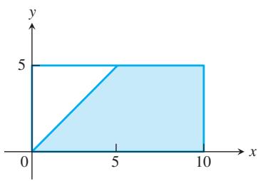
FIGURE 14.45 The pair of random variables X and Y take values anywhere in this rectangle with equal probability. In the shaded region we have X > Y.
To compute the probability that X > Y, we integrate the joint probability density function f over the region in the rectangle where X > Y. This region is bounded on the left by the line x = y and on the right by the line x = 10. An integral over this region has limits of integration given by
There is a 75% probability that the first number is larger than the second.
EXAMPLE 6 Using the joint probability density function
find the probability that 1 < X < 2 and 2 < Y < 3.
Solution
There is slightly less than a 2% probability that X and Y fall within these bounds.
Means and Expected Values
The mean, or expected value, of a random variable is (Appendix A.8)
When X and Y have joint probability density function f, the expected value of X and the expected value of Y are
These indicate the average value expected for each of X and Y. The expected values
EXAMPLE 7 Find the expected values
Solution For the joint probability density function in Example 5, we compute
and
The expected value of X is 5 and that of Y is 2.5.
EXERCISES 14.6
Plates of Constant Density
-
Finding a center of mass Find the center of mass of a thin plate of density
𝛿 = 3 𝑦 = 2 − 𝑥 2 -
Finding moments of inertia Find the moments of inertia about the coordinate axes of a thin rectangular plate of constant density
𝛿 g m / c m 2 𝑥 = 3 𝑦 = 3 -
Finding a centroid Find the centroid of the region in the first quadrant bounded by the x-axis, the parabola
𝑦 2 = 2 𝑥 𝑥 + 𝑦 = 4 -
Finding a centroid Find the centroid of the triangular region cut from the first quadrant by the line
𝑥 + 𝑦 = 3 -
Finding a centroid Find the centroid of the region cut from the first quadrant by the circle
𝑥 2 + 𝑦 2 = 𝑎 2 -
Finding a centroid Find the centroid of the region between the x-axis and the arch
𝑦 = s i n 𝑥 , 0 ≤ 𝑥 ≤ 𝜋 -
Finding moments of inertia Find the moment of inertia about the
𝑥 𝛿 = 1 g m / c m 2 𝑥 2 + 𝑦 2 = 4 𝐼 𝑦 𝐼 0 -
Finding a moment of inertia Find the moment of inertia with respect to the y-axis of a thin sheet of constant density
𝛿 = 1 𝑔 𝑚 / 𝑐 𝑚 2 𝑦 = ( s i n 2 𝑥 ) / 𝑥 2 𝜋 ≤ 𝑥 ≤ 2 𝜋 -
The centroid of an infinite region Find the centroid of the infinite region in the second quadrant enclosed by the coordinate axes and the curve
𝑦 = 𝑒 𝑥 -
The first moment of an infinite plate Find the first moment about the y-axis of a thin plate of density
𝛿 ( 𝑥 , 𝑦 ) = 1 𝑦 = 𝑒 − 𝑥 2 / 2
Plates with Varying Density
-
Finding a moment of inertia Find the moment of inertia about the x-axis of a thin plate bounded by the parabola
𝑥 = 𝑦 − 𝑦 2 𝑥 + 𝑦 = 0 𝛿 ( 𝑥 , 𝑦 ) = 𝑥 + 𝑦 -
Finding mass Find the mass of a thin plate occupying the smaller region cut from the ellipse
𝑥 2 + 4 𝑦 2 = 1 2 𝑥 = 4 𝑦 2 𝛿 ( 𝑥 , 𝑦 ) = 5 𝑥 k g / m 2 -
Finding a center of mass Find the center of mass of a thin triangular plate bounded by the
𝑦 𝑦 = 𝑥 𝑦 = 2 − 𝑥 𝛿 ( 𝑥 , 𝑦 ) = 6 𝑥 + 3 𝑦 + 3 -
Finding a center of mass and moment of inertia Find the center of mass and moment of inertia about the x-axis of a thin plate bounded by the curves
𝑥 = 𝑦 2 𝑥 = 2 𝑦 − 𝑦 2 ( 𝑥 , 𝑦 ) 𝛿 ( 𝑥 , 𝑦 ) = 𝑦 + 1 -
Center of mass, moment of inertia Find the center of mass and the moment of inertia about the y-axis of a thin rectangular plate cut from the first quadrant by the lines x = 6 and y = 1 if
𝛿 ( 𝑥 , 𝑦 ) = 𝑥 + 𝑦 + 1 -
Center of mass, moment of inertia Find the center of mass and the moment of inertia about the
𝑦 𝑦 = 1 𝑦 = 𝑥 2 𝛿 ( 𝑥 , 𝑦 ) = 𝑦 + 1 -
Center of mass, moment of inertia Find the center of mass and the moment of inertia about the
𝑦 𝑥 𝑥 = ± 1 𝑦 = 𝑥 2 𝛿 ( 𝑥 , 𝑦 ) = 7 𝑦 + 1 -
Center of mass, moments of inertia Find the center of mass and the moments of inertia about the
𝑥 𝑥 = 0 𝑥 = 2 0 𝑦 = − 1 𝑦 = 1 𝛿 ( 𝑥 , 𝑦 ) = 1 + ( 𝑥 / 2 0 ) -
Center of mass, moments of inertia Find the center of mass, the moment of inertia about the coordinate axes, and the polar moment of inertia of a thin triangular plate bounded by the lines y = x, y = -x, and y = 1 if
𝛿 ( 𝑥 , 𝑦 ) = 𝑦 + 1 k g / m 2 -
Center of mass, moments of inertia Repeat Exercise 19 for
𝛿 ( 𝑥 , 𝑦 ) = 3 𝑥 2 + 1 𝑘 𝑔 / 𝑚 2
Solids with Constant Density
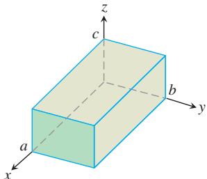
- Moments of inertia Find the moments of inertia of the rectangular box of constant density
𝛿 ( 𝑥 , 𝑦 , 𝑧 ) = 1 𝐼 𝑥 𝐼 𝑦 𝐼 𝑧
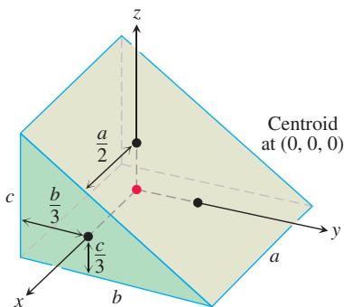
- Moments of inertia The coordinate axes in the figure run through the centroid of a solid wedge parallel to the labeled edges. Find
𝐼 𝑥 𝐼 𝑦 𝐼 𝑧 𝛿 ( 𝑥 , 𝑦 , 𝑧 ) = 1
-
Center of mass and moments of inertia A solid “trough” of constant density
𝛿 ( 𝑥 , 𝑦 , 𝑧 ) = 1 𝑧 = 4 𝑦 2 -
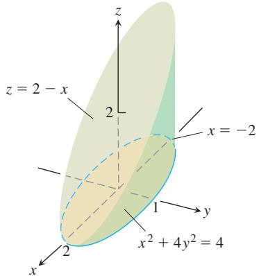
Center of mass A solid of constant density is bounded below by the plane z = 0, on the sides by the elliptical cylinder
𝑥 2 + 4 𝑦 2 = 4
a. Find
b. Evaluate the integral
using integral tables to carry out the final integration with respect to
- a. Center of mass Find the center of mass of a solid of constant density bounded below by the paraboloid
𝑧 = 𝑥 2 + 𝑦 2
b. Find the plane z = c that divides the solid into two parts of equal volume. This plane does not pass through the center of mass.
-
Moments A solid cube of constant density
𝛿 ( 𝑥 , 𝑦 , 𝑧 ) = 1 𝑥 = ± 1 𝑧 = ± 1 -
Moment of inertia about a line A wedge like the one in Exercise 22 has
𝑎 = 4 𝑏 = 6 𝑐 = 3 𝛿 ( 𝑥 , 𝑦 , 𝑧 ) = 1 ( 𝑥 , 𝑦 , 𝑧 ) 𝐿 𝑧 = 0 𝑦 = 6 𝑟 2 = ( 𝑦 − 6 ) 2 + 𝑧 2 𝐿 -
Moment of inertia about a line A wedge like the one in Exercise 22 has
𝑎 = 4 𝑏 = 6 𝑐 = 3 𝛿 ( 𝑥 , 𝑦 , 𝑧 ) = 1 ( 𝑥 , 𝑦 , 𝑧 ) 𝐿 𝑥 = 4 𝑦 = 0 𝑟 2 = ( 𝑥 − 4 ) 2 + 𝑦 2 𝐿
Solids with Varying Density
In Exercises 29 and 30, find
a. the mass of the solid. b. the center of mass.
-
A solid region in the first octant is bounded by the coordinate planes and the plane
𝑥 + 𝑦 + 𝑧 = 2 𝛿 ( 𝑥 , 𝑦 , 𝑧 ) = 2 𝑥 g m / c m 3 -
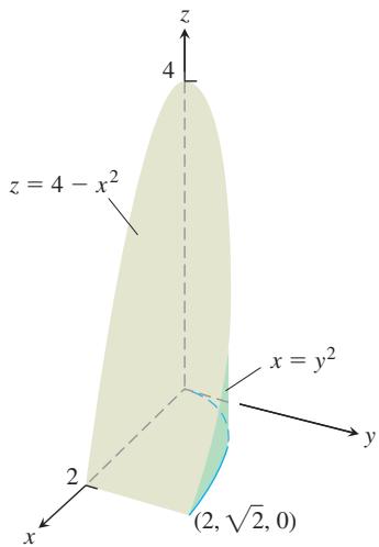
A solid in the first octant is bounded by the planes y = 0 and z = 0 and by the surfaces
𝑧 = 4 − 𝑥 2 𝑥 = 𝑦 2 𝛿 ( 𝑥 , 𝑦 , 𝑧 ) = 𝑘 𝑥 𝑦
In Exercises 31 and 32, find
a. the mass of the solid.
b. the center of mass.
c. the moments of inertia about the coordinate axes.
-
A solid cube in the first octant is bounded by the coordinate planes and by the planes x = 1, y = 1, and z = 1. The density of the cube is
𝛿 ( 𝑥 , 𝑦 , 𝑧 ) = 𝑥 + 𝑦 + 𝑧 + 1 -
A wedge like the one in Exercise 22 has dimensions
𝑎 = 2 𝑏 = 6 𝑐 = 3 𝛿 ( 𝑥 , 𝑦 , 𝑧 ) = 𝑥 + 1 ( 0 , 0 , 0 ) -
Mass Find the mass of the solid bounded by the planes
𝑥 + 𝑧 = 1 𝑦 = √ 𝑧 𝛿 ( 𝑥 , 𝑦 , 𝑧 ) = 2 𝑦 + 5 k g / m 3 -
Mass Find the mass of the solid region bounded by the parabolic surfaces
𝑧 = 1 6 − 2 𝑥 2 − 2 𝑦 2 𝑧 = 2 𝑥 2 + 2 𝑦 2 𝛿 ( 𝑥 , 𝑦 , 𝑧 ) = √ 𝑥 2 + 𝑦 2
Theory and Examples
The Parallel Axis Theorem Let
As in the two-dimensional case, the theorem gives a quick way to calculate one moment when the other moment and the mass are known.
- Proof of the Parallel Axis Theorem
a. Show that the first moment of a body in space about any plane through the body’s center of mass is zero. (Hint: Place the body’s center of mass at the origin and let the plane be the yz-plane. What does the formula
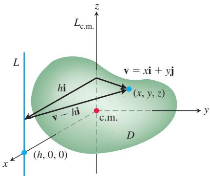
b. To prove the Parallel Axis Theorem, place the body with its center of mass at the origin, with the line
Expand the integrand in this integral and complete the proof.
-
The moment of inertia about a diameter of a solid sphere of constant density and radius
𝑎 ( 2 / 5 ) 𝑚 𝑎 2 𝑚 -
The moment of inertia of the solid in Exercise 21 about the
𝑧 𝐼 𝑧 = 𝑎 𝑏 𝑐 ( 𝑎 2 + 𝑏 2 ) / 3
a. Use Equation (2) to find the moment of inertia of the solid about the line parallel to the
b. Use Equation (2) and the result in part (a) to find the moment of inertia of the solid about the line x = 0, y = 2b.
- If
𝑎 = 𝑏 = 6 𝑐 = 4 𝑥 𝐼 𝑥 = 2 0 8 𝑦 = 4 𝑧 = − 4 / 3
Joint Probability Density Functions
For Exercises 39–42, verify that f gives a joint probability density function. Then find the expected values
-
𝑓 ( 𝑥 , 𝑦 ) = { 𝑥 + 𝑦 , i f 0 ≤ 𝑥 ≤ 1 a n d 0 ≤ 𝑦 ≤ 1 , 0 , o t h e r w i s e . -
𝑓 ( 𝑥 , 𝑦 ) = { 4 𝑥 𝑦 , i f 0 ≤ 𝑥 ≤ 1 a n d 0 ≤ 𝑦 ≤ 1 , 0 , o t h e r w i s e . -
𝑓 ( 𝑥 , 𝑦 ) = { 6 𝑥 2 𝑦 , i f 0 ≤ 𝑥 ≤ 1 a n d 0 ≤ 𝑦 ≤ 1 , 0 , o t h e r w i s e . -
𝑓 ( 𝑥 , 𝑦 ) = { 3 2 ( 𝑥 2 + 𝑦 2 ) , i f 0 ≤ 𝑥 ≤ 1 a n d 0 ≤ 𝑦 ≤ 1 , 0 , o t h e r w i s e . -
Suppose that
𝑓 0 ≤ 𝑥 < 2 0 ≤ 𝑦 < 3 𝑓 𝑋 < 𝑌 -
The following formula defines a joint probability density function. What is the value of C? What are the expected values
𝜇 𝑋 𝜇 𝑌
14.7 Triple Integrals in Cylindrical and Spherical Coordinates
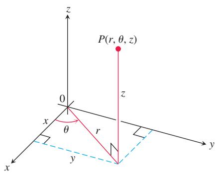
FIGURE 14.46 The cylindrical coordinates of a point in space are r,
When a calculation in physics, engineering, or geometry involves a cylinder, cone, or sphere, we can often simplify our work by using cylindrical or spherical coordinates, which are introduced in this section. The procedure for transforming to these coordinates and evaluating the resulting triple integrals is similar to the transformation to polar coordinates in the plane discussed in Section 14.4.
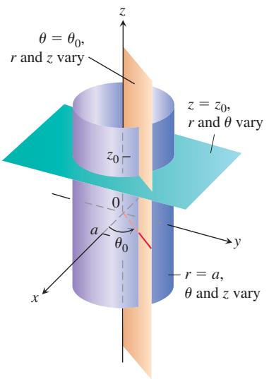
FIGURE 14.47 Constant-coordinate equations in cylindrical coordinates yield cylinders and planes.
Integration in Cylindrical Coordinates
We obtain cylindrical coordinates for space by combining polar coordinates in the xy-plane with the usual z-axis. This assigns to every point in space coordinate triples of the form
DEFINITION Cylindrical coordinates represent a point P in space by ordered triples
in which ( 𝑟 , 𝜃 , 𝑧 )
r and
are polar coordinates for the vertical projection of P on the xy-plane, with 𝜃 , and 𝑟 ≥ 0 z is the rectangular vertical coordinate.
The values of
Equations Relating Rectangular
In cylindrical coordinates, the equation r = a describes not just a circle in the xy-plane but an entire cylinder about the z-axis (Figure 14.47). The z-axis is given by r = 0. The equation
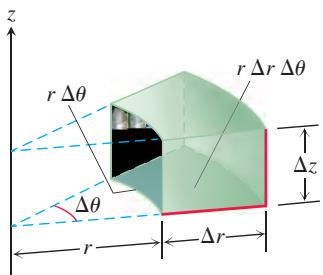
FIGURE 14.48 In cylindrical coordinates the volume of the wedge is approximated by the product
Volume Differential in Cylindrical Coordinates
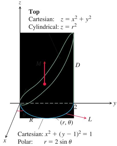
FIGURE 14.49 Finding the limits of integration for evaluating an integral in cylindrical coordinates (Example 1).
Cylindrical coordinates are good for describing cylinders whose axes run along the z-axis and planes that either contain the z-axis or lie perpendicular to the z-axis. Surfaces like these have equations of constant coordinate value:
When computing triple integrals over a solid region D in cylindrical coordinates, we partition the region into n small cylindrical wedges, rather than into rectangular boxes. In the kth cylindrical wedge,
For a point
The triple integral of a function
Triple integrals in cylindrical coordinates are then evaluated as iterated integrals, as in the following example. Although the definition of cylindrical coordinates makes sense without any restrictions on
EXAMPLE 1 Find the limits of integration in cylindrical coordinates for integrating a function
Solution The base of
The region is sketched in Figure 14.49.
We find the limits of integration, starting with the
Next we find the r-limits of integration. A ray L through
Finally, we find the
Example 1 illustrates a good procedure for finding limits of integration in cylindrical coordinates. The procedure is summarized as follows.
How to Integrate in Cylindrical Coordinates
To evaluate
over a solid region D in space in cylindrical coordinates, integrating first with respect to z, then with respect to r, and finally with respect to
- Sketch. Sketch the solid region D along with its projection R on the xy-plane. Label the surfaces and curves that bound D and R.
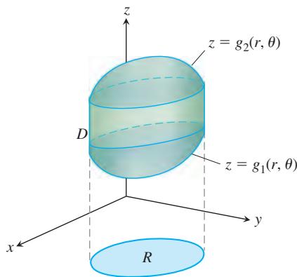
- Find the
𝑧 𝑀 ( 𝑟 , 𝜃 ) 𝑅 𝑧 𝑧 𝑀 𝐷 𝑧 = 𝑔 1 ( 𝑟 , 𝜃 ) 𝑧 = 𝑔 2 ( 𝑟 , 𝜃 ) 𝑧
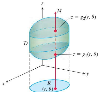
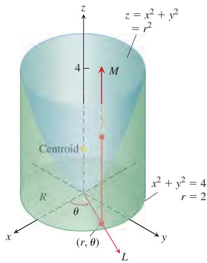
FIGURE 14.50 Example 2 shows how to find the centroid of this solid.
- Find the r-limits of integration. Draw a ray L through
( 𝑟 , 𝜃 ) 𝑟 = ℎ 1 ( 𝜃 ) 𝑟 = ℎ 2 ( 𝜃 )
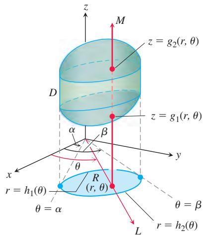
- Find the
𝜃 𝜃 𝜃 = 𝛼 𝜃 = 𝛽 𝜃
EXAMPLE 2 Find the centroid (
Solution We sketch the solid, bounded above by the paraboloid
The solid’s centroid
To find the limits of integration for the mass and moment integrals, we continue with the four basic steps. We completed our initial sketch. The remaining steps give the limits of integration.
The z-limits. A line M through a typical point
The
The
The value of
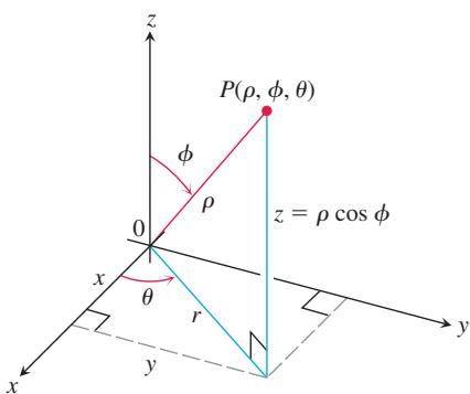
FIGURE 14.51 The spherical coordinates
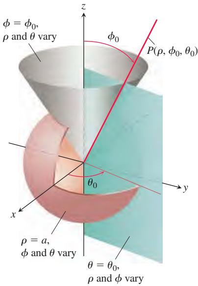
FIGURE 14.52 Constant-coordinate equations in spherical coordinates yield spheres, single cones, and half-planes.
Therefore,
and the centroid is
Spherical Coordinates and Integration
Spherical coordinates locate points in space with two angles and one distance, as shown in Figure 14.51. The first coordinate,
DEFINITION Spherical coordinates represent a point P in space by ordered triples
in which ( 𝜌 , 𝜙 , 𝜃 )
is the distance from P to the origin ( 𝜌 ). 𝜌 ≥ 0
is the angle 𝜙 makes with the positive z-axis ( ⟶ 𝑂 𝑃 ). 0 ≤ 𝜙 ≤ 𝜋
is the angle from cylindrical coordinates. 𝜃
On maps of Earth,
The equation
Equations Relating Spherical Coordinates to Cartesian and Cylindrical Coordinates
EXAMPLE 3 Find a spherical coordinate equation for the sphere
Solution We use Equations (1) to substitute for x, y, and z:
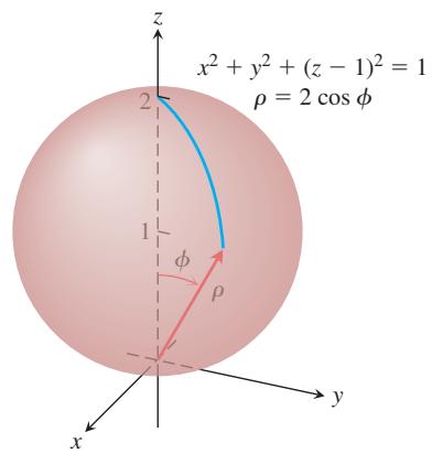
FIGURE 14.53 The sphere in Example 3.
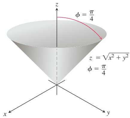
FIGURE 14.54 The cone in Example 4.
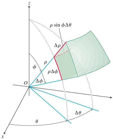
FIGURE 14.55 In spherical coordinates we use the volume of a spherical wedge, which closely approximates that of a rectangular box.
Volume Differential in Spherical Coordinates
The angle
EXAMPLE 4 Find a spherical coordinate equation for the cone
Solution 1 Use geometry. The cone is symmetric with respect to the z-axis and cuts the first quadrant of the yz-plane along the line z = y. The angle between the cone and the positive z-axis is therefore
Solution 2 Use algebra. If we use Equations (1) to substitute for x, y, and z, we obtain the same result:
Spherical coordinates are useful for describing spheres centered at the origin, half-planes hinged along the z-axis, and cones whose vertices lie at the origin and whose axes lie along the z-axis. Surfaces like these have equations of constant coordinate value:
When computing triple integrals over a solid region D in spherical coordinates, we partition the region into n spherical wedges. The size of the kth spherical wedge, which contains a point
The corresponding Riemann sum for a function
As the norm of a partition approaches zero, and the spherical wedges get smaller, the limit of the Riemann sums is the triple integral:
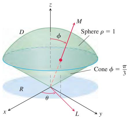
FIGURE 14.56 The ice cream cone in Example 5.
To evaluate integrals in spherical coordinates, we usually integrate first with respect to
How to Integrate in Spherical Coordinates
To evaluate
over a solid region D in space in spherical coordinates, integrating first with respect to
- Sketch. Sketch the solid region D along with its projection R on the xy-plane. Label the surfaces that bound D.
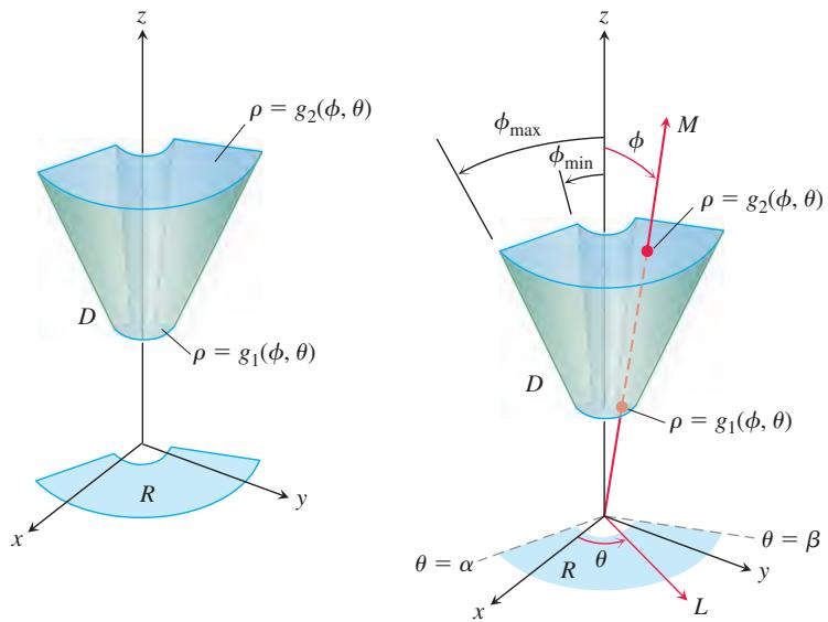
-
Find the
𝜌 𝜙 𝜃 𝜌 𝜌 = 𝑔 1 ( 𝜙 , 𝜃 ) 𝜌 = 𝑔 2 ( 𝜙 , 𝜃 ) 𝜌 -
Find the
𝜙 𝜃 𝜙 𝜙 = 𝜙 𝑚 𝑖 𝑛 𝜙 = 𝜙 𝑚 𝑎 𝑥 𝜙 𝜃 -
Find the
𝜃 𝜃 𝛼 𝛽 𝜃
EXAMPLE 5 Find the volume of the “ice cream cone” D bounded above by the sphere
Solution The volume is
To find the limits of integration for evaluating the integral, we begin by sketching D and its projection R on the xy-plane (Figure 14.56).
The
The
The
EXAMPLE 6 A solid of constant density
Solution In rectangular coordinates, the moment is
In spherical coordinates,
For the region
Coordinate Conversion Formulas
CYLINDRICAL TO
SPHERICAL TO
SPHERICAL TO
RECTANGULAR
RECTANGULAR
CYLINDRICAL
Corresponding formulas for dV in triple integrals:
In the next section we offer a more general procedure for determining dV in cylindrical and spherical coordinates. The results, of course, will be the same.
EXERCISES 14.7
In Exercises 1–12, sketch the region described by the following cylindrical coordinates in three-dimensional space.
-
𝑟 = 2 -
𝜃 = 𝜋 4 -
𝑧 = − 1 -
𝑧 = 𝑟 -
𝑟 = 𝜃 -
𝑧 = 𝑟 s i n 𝜃 -
𝑟 2 + 𝑧 2 = 4 -
1 ≤ 𝑟 ≤ 2 , 0 ≤ 𝜃 ≤ 𝜋 3 -
𝑟 ≤ 𝑧 ≤ √ 9 − 𝑟 2 -
0 ≤ 𝑟 ≤ 2 s i n 𝜃 , 1 ≤ 𝑧 ≤ 3 -
0 ≤ 𝑟 ≤ 4 c o s 𝜃 , 0 ≤ 𝜃 ≤ 𝜋 2 , 0 ≤ 𝑧 ≤ 5 -
0 ≤ 𝑟 ≤ 3 , − 𝜋 2 ≤ 𝜃 ≤ 𝜋 2 , 0 ≤ 𝑧 ≤ 𝑟 c o s 𝜃
In Exercises 13–22, sketch the region described by the following spherical coordinates in three-dimensional space.
-
𝜌 = 3 -
𝜙 = 𝜋 6 -
𝜃 = 2 3 𝜋 -
𝜌 = c s c 𝜙 -
𝜌 c o s 𝜙 = 4 -
1 ≤ 𝜌 ≤ 2 s e c 𝜙 , 0 ≤ 𝜙 ≤ 𝜋 4 -
0 ≤ 𝜌 ≤ 3 c s c 𝜙 -
0 ≤ 𝜌 ≤ 1 𝜋 2 ≤ 𝜙 ≤ 𝜋 0 ≤ 𝜃 ≤ 𝜋 -
0 ≤ 𝜌 c o s 𝜃 s i n 𝜙 ≤ 2 , 0 ≤ 𝜌 s i n 𝜃 s i n 𝜙 ≤ 3 , 0 ≤ 𝜌 c o s 𝜙 ≤ 4 -
4 s e c 𝜙 ≤ 𝜌 ≤ 5 , 0 ≤ 𝜙 ≤ 𝜋 2
Evaluating Integrals in Cylindrical Coordinates
Evaluate the cylindrical coordinate integrals in Exercises 23-28.
-
∫ 2 𝜋 0 ∫ 1 0 ∫ √ 2 − 𝑟 2 𝑟 𝑟 𝑑 𝑧 𝑑 𝑟 𝑑 𝜃 -
∫ 2 𝜋 0 ∫ 3 0 ∫ √ 1 8 − 𝑟 2 𝑟 2 / 3 𝑟 𝑑 𝑧 𝑑 𝑟 𝑑 𝜃 -
∫ 2 𝜋 0 ∫ 𝜃 / 2 𝜋 0 ∫ 3 + 2 4 𝑟 2 0 𝑟 𝑑 𝑧 𝑑 𝑟 𝑑 𝜃 -
∫ 𝜋 0 ∫ 𝜃 / 𝜋 0 ∫ 3 √ 4 − 𝑟 2 − √ 4 − 𝑟 2 𝑧 𝑟 𝑑 𝑧 𝑑 𝑟 𝑑 𝜃 -
∫ 2 𝜋 0 ∫ 1 0 ∫ 1 / √ 2 − 𝑟 2 𝑟 3 𝑟 𝑑 𝑧 𝑑 𝑟 𝑑 𝜃 -
∫ 2 𝜋 0 ∫ 1 0 ∫ 1 / 2 − 1 / 2 ( 𝑟 2 s i n 2 𝜃 + 𝑧 2 ) 𝑟 𝑑 𝑧 𝑑 𝑟 𝑑 𝜃
The integrals we have seen so far suggest that there are preferred orders of integration for cylindrical coordinates, but other orders usually work well and are occasionally easier to evaluate. Evaluate the integrals in Exercises 29–32.
-
∫ 2 𝜋 0 ∫ 3 0 ∫ 𝑧 / 3 0 𝑟 3 𝑑 𝑟 𝑑 𝑧 𝑑 𝜃 -
∫ 1 − 1 ∫ 2 𝜋 0 ∫ 1 + c o s 𝜃 0 4 𝑟 𝑑 𝑟 𝑑 𝜃 𝑑 𝑧 -
∫ 1 0 ∫ √ 𝑧 0 ∫ 2 𝜋 0 ( 𝑟 2 c o s 2 𝜃 + 𝑧 2 ) 𝑟 𝑑 𝜃 𝑑 𝑟 𝑑 𝑧 -
∫ 2 0 ∫ √ 4 − 𝑟 2 𝑟 − 2 ∫ 2 𝜋 0 ( 𝑟 s i n 𝜃 + 1 ) 𝑟 𝑑 𝜃 𝑑 𝑧 𝑑 𝑟 -
Let
𝐷 𝑧 = 0 𝑥 2 + 𝑦 2 + 𝑧 2 = 4 𝑥 2 + 𝑦 2 = 1 𝐷 𝑑 𝑧 𝑑 𝑟 𝑑 𝜃 𝑑 𝑟 𝑑 𝑧 𝑑 𝜃 𝑑 𝜃 𝑑 𝑧 𝑑 𝑟 -
Let D be the solid region bounded below by the cone
𝑧 = √ 𝑥 2 + 𝑦 2 𝑧 = 2 − 𝑥 2 − 𝑦 2
Finding Iterated Integrals in Cylindrical Coordinates
- Give the limits of integration for evaluating the integral
as an iterated integral over the solid region D that is bounded below by the plane z = 0, on the side by the cylinder
- Convert the integral
to an equivalent integral in cylindrical coordinates and evaluate the result.
In Exercises 37–42, set up the iterated integral for evaluating
- D is the right circular cylinder whose base is the circle
𝑟 = 2 s i n 𝜃
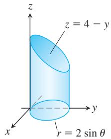
- D is the right circular cylinder whose base is the circle
𝑟 = 3 c o s 𝜃
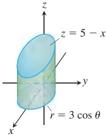
- D is the solid right cylinder whose base is the region in the xy-plane that lies inside the cardioid
𝑟 = 1 + c o s 𝜃
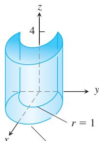
- D is the solid right cylinder whose base is the region between the circles
𝑟 = c o s 𝜃 𝑟 = 2 c o s 𝜃
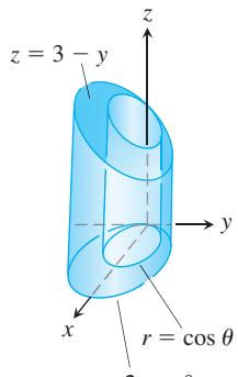
- D is the right prism whose base is the triangle in the xy-plane bounded by the x-axis and the lines y = x and x = 1 and whose top lies in the plane z = 2 - y.
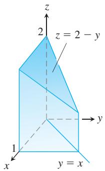
- D is the right prism whose base is the triangle in the xy-plane bounded by the y-axis and the lines y = x and y = 1 and whose top lies in the plane z = 2 - x.
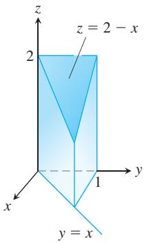
Evaluating Integrals in Spherical Coordinates
Evaluate the spherical coordinate integrals in Exercises 43-48.
-
∫ 𝜋 0 ∫ 𝜋 0 ∫ 2 s i n 𝜙 0 𝜌 2 s i n 𝜙 𝑑 𝜌 𝑑 𝜙 𝑑 𝜃 -
∫ 2 𝜋 0 ∫ 𝜋 / 4 0 ∫ 2 0 ( 𝜌 c o s 𝜙 ) 𝜌 2 s i n 𝜙 𝑑 𝜌 𝑑 𝜙 𝑑 𝜃 -
∫ 2 𝜋 0 ∫ 𝜋 0 ∫ ( 1 − c o s 𝜙 ) / 2 0 𝜌 2 s i n 𝜙 𝑑 𝜌 𝑑 𝜙 𝑑 𝜃 -
∫ 3 𝜋 / 2 0 ∫ 𝜋 0 ∫ 1 0 5 𝜌 3 s i n 3 𝜙 𝑑 𝜌 𝑑 𝜙 𝑑 𝜃 -
∫ 2 𝜋 0 ∫ 𝜋 / 3 0 ∫ 2 s e c 𝜙 3 𝜌 2 s i n 𝜙 𝑑 𝜌 𝑑 𝜙 𝑑 𝜃 -
∫ 2 𝜋 0 ∫ 𝜋 / 4 0 ∫ s e c 𝜙 0 ( 𝜌 c o s 𝜙 ) 𝜌 2 s i n 𝜙 𝑑 𝜌 𝑑 𝜙 𝑑 𝜃
Changing the Order of Integration in Spherical Coordinates The previous integrals suggest there are preferred orders of integration for spherical coordinates, but other orders give the same value and are occasionally easier to evaluate. Evaluate the integrals in Exercises 49–52.
-
∫ 2 0 ∫ 0 − 𝜋 ∫ 𝜋 / 2 𝜋 / 4 𝜌 3 s i n 2 𝜙 𝑑 𝜙 𝑑 𝜃 𝑑 𝜌 -
∫ 𝜋 / 3 𝜋 / 6 ∫ 2 c s c 𝜙 c s c 𝜙 ∫ 2 𝜋 0 𝜌 2 s i n 𝜙 𝑑 𝜃 𝑑 𝜌 𝑑 𝜙 -
∫ 1 0 ∫ 𝜋 0 ∫ 𝜋 / 4 0 1 2 𝜌 s i n 3 𝜙 𝑑 𝜙 𝑑 𝜃 𝑑 𝜌 -
∫ 𝜋 / 2 𝜋 / 6 ∫ 𝜋 / 2 − 𝜋 / 2 ∫ 2 c s c 𝜙 5 𝜌 4 s i n 3 𝜙 𝑑 𝜌 𝑑 𝜃 𝑑 𝜙 -
Let
𝐷 𝐷
a.
b.
- Let D be the solid region bounded below by the cone
𝑧 = √ 𝑥 2 + 𝑦 2
a.
b.
Finding Iterated Integrals in Spherical Coordinates
In Exercises 55–60, (a) find the spherical coordinate limits for the integral that calculates the volume of the given solid and then (b) evaluate the integral.
- The solid between the sphere
𝜌 = c o s 𝜙 𝜌 = 2 , 𝑧 ≥ 0
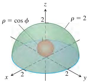
- The solid bounded below by the hemisphere
𝜌 = 1 , 𝑧 ≥ 0 𝜌 = 1 + c o s 𝜙
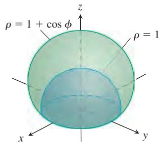
-
The solid enclosed by the surface
𝜌 = 1 − c o s 𝜙 -
The upper portion cut from the solid in Exercise 57 by the xy-plane
-
The solid bounded below by the sphere
𝜌 = 2 c o s 𝜙 𝑧 = √ 𝑥 2 + 𝑦 2
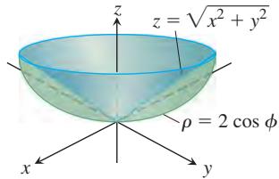
- The solid bounded below by the xy-plane, on the sides by the sphere
𝜌 = 2 𝜙 = 𝜋 / 3
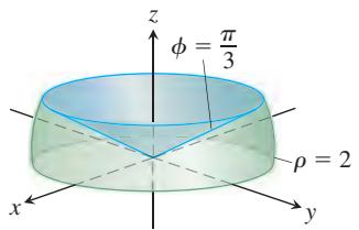
Finding Triple Integrals
-
Set up triple integrals for the volume of the sphere
𝜌 = 2 -
Let D be the solid region in the first octant that is bounded below by the cone
𝜙 = 𝜋 / 4 𝜌 = 3 -
Let D be the smaller cap cut from a solid ball of radius 2 units by a plane 1 unit from the center of the sphere. Express the volume of D as an iterated triple integral in (a) spherical, (b) cylindrical, and (c) rectangular coordinates. Then (d) find the volume by evaluating one of the three triple integrals.
-
Let
𝐷 𝑥 2 + 𝑦 2 + 𝑧 2 ≤ 1 𝑧 ≥ 0 𝛿 ( 𝑥 , 𝑦 , 𝑧 ) = 1 𝐼 𝑧 𝐼 𝑧
Volumes
Find the volumes of the solids in Exercises 65–70.
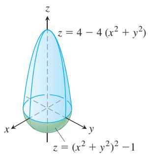
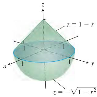
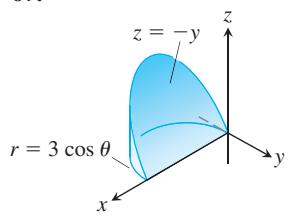
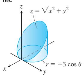
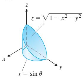
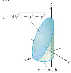
-
Ball and cones Find the volume of the portion of the ball
𝜌 ≤ 𝑎 𝜙 = 𝜋 / 3 𝜙 = 2 𝜋 / 3 -
Ball and half-planes Find the volume of the region cut from the ball
𝜌 ≤ 𝑎 𝜃 = 0 𝜃 = 𝜋 / 6 -
Ball and plane Find the volume of the smaller region cut from the ball
𝜌 ≤ √ 2 -
Cone and planes Find the volume of the solid enclosed by the cone
𝑧 = √ 𝑥 2 + 𝑦 2 -
Cylinder and paraboloid Find the volume of the solid region bounded below by the plane z = 0, laterally by the cylinder
𝑥 2 + 𝑦 2 = 1 𝑧 = 𝑥 2 + 𝑦 2 -
Cylinder and paraboloids Find the volume of the solid region bounded below by the paraboloid
𝑧 = 𝑥 2 + 𝑦 2 𝑥 2 + 𝑦 2 = 1 𝑧 = 𝑥 2 + 𝑦 2 + 1 -
Cylinder and cones Find the volume of the solid cut from the thick-walled cylinder
1 ≤ 𝑥 2 + 𝑦 2 ≤ 2 𝑧 = ± √ 𝑥 2 + 𝑦 2 -
Sphere and cylinder Find the volume of the solid region that lies inside the sphere
𝑥 2 + 𝑦 2 + 𝑧 2 = 2 𝑥 2 + 𝑦 2 = 1 -
Cylinder and planes Find the volume of the solid region enclosed by the cylinder
𝑥 2 + 𝑦 2 = 4 𝑦 + 𝑧 = 4 -
Cylinder and planes Find the volume of the solid region enclosed by the cylinder
𝑥 2 + 𝑦 2 = 4 𝑥 + 𝑦 + 𝑧 = 4 -
Region trapped by paraboloids Find the volume of the solid region bounded above by the paraboloid
𝑧 = 5 − 𝑥 2 − 𝑦 2 𝑧 = 4 𝑥 2 + 4 𝑦 2 -
Paraboloid and cylinder Find the volume of the solid region bounded above by the paraboloid
𝑧 = 9 − 𝑥 2 − 𝑦 2 𝑥 2 + 𝑦 2 = 1 -
Cylinder and sphere Find the volume of the region cut from the solid cylinder
𝑥 2 + 𝑦 2 ≤ 1 𝑥 2 + 𝑦 2 + 𝑧 2 = 4 -
Sphere and paraboloid Find the volume of the solid region bounded above by the sphere
𝑥 2 + 𝑦 2 + 𝑧 2 = 2 𝑧 = 𝑥 2 + 𝑦 2
Average Values
-
Find the average value of the function
𝑓 ( 𝑟 , 𝜃 , 𝑧 ) = 𝑟 𝑟 = 1 𝑧 = − 1 𝑧 = 1 -
Find the average value of the function
𝑓 ( 𝑟 , 𝜃 , 𝑧 ) = 𝑟 𝑟 2 + 𝑧 2 = 1 𝑥 2 + 𝑦 2 + 𝑧 2 = 1 -
Find the average value of the function
𝑓 ( 𝜌 , 𝜙 , 𝜃 ) = 𝜌 𝜌 ≤ 1 -
Find the average value of the function
𝑓 ( 𝜌 , 𝜙 , 𝜃 ) = 𝜌 c o s 𝜙 𝜌 ≤ 1 , 0 ≤ 𝜙 ≤ 𝜋 / 2
Masses, Moments, and Centroids
-
Center of mass A solid of constant density is bounded below by the plane z = 0, above by the cone z = r,
𝑟 ≥ 0 -
Centroid Find the centroid of the solid region in the first octant that is bounded above by the cone
𝑧 = √ 𝑥 2 + 𝑦 2 𝑥 2 + 𝑦 2 = 4 -
Centroid Find the centroid of the solid in Exercise 60.
-
Centroid Find the centroid of the solid bounded above by the sphere
𝜌 = 𝑎 𝜙 = 𝜋 / 4 -
Centroid Find the centroid of the solid region that is bounded above by the surface
𝑧 = √ 𝑟 -
Centroid Find the centroid of the region cut from the solid ball
𝑟 2 + 𝑧 2 ≤ 1 𝜃 = − 𝜋 / 3 𝑟 ≥ 0 𝜃 = 𝜋 / 3 𝑟 ≥ 0 -
Moment of inertia of solid cone Find the moment of inertia of a solid right circular cone of base radius 1 and height 1 about an axis through the vertex parallel to the base if the density is
𝛿 = 1 -
Moment of inertia of ball Find the moment of inertia of a ball of radius
𝑎 𝛿 = 1 -
Moment of inertia of solid cone Find the moment of inertia of a solid right circular cone of base radius
𝑎 ℎ 𝛿 = 1 𝑧 -
Variable density A solid is bounded on the top by the paraboloid
𝑧 = 𝑟 2 𝑧 = 0 𝑟 = 1 𝑧 𝛿 ( 𝑟 , 𝜃 , 𝑧 ) = 𝑧 𝛿 ( 𝑟 , 𝜃 , 𝑧 ) = 𝑟 -
Variable density A solid is bounded below by the cone
𝑧 = √ 𝑥 2 + 𝑦 2 𝑧 = 1 𝑧
-
Variable density A solid ball is bounded by the sphere
𝜌 = 𝑎 𝑧
a.𝛿 ( 𝜌 , 𝜙 , 𝜃 ) = 𝜌 2 𝛿 ( 𝜌 , 𝜙 , 𝜃 ) = 𝑟 = 𝜌 s i n 𝜙 -
Centroid of solid semi-ellipsoid Show that the centroid of the solid semi-ellipsoid of revolution
( 𝑟 2 / 𝑎 2 ) + ( 𝑧 2 / ℎ 2 ) ≤ 1 𝑧 ≥ 0 -
Centroid of solid cone Show that the centroid of a solid right circular cone is one-fourth of the way from the base to the vertex. (In general, the centroid of a solid cone or pyramid is one-fourth of the way from the centroid of the base to the vertex.)
-
Density of center of a planet A planet is in the shape of a sphere of radius R and total mass M with spherically symmetric density distribution that increases linearly as one approaches its center. What is the density at the center of this planet if the density at its edge (surface) is taken to be zero?
-
Mass of planet’s atmosphere A spherical planet of radius
𝑅 𝜇 = 𝜇 0 𝑒 − 𝑐 ℎ ℎ 𝜇 0 𝑐
Theory and Examples
- Vertical planes in cylindrical coordinates
a. Show that planes perpendicular to the x-axis have equations of the form
b. Show that planes perpendicular to the y-axis have equations of the form
-
(Continuation of Exercise 105.) Find an equation of the form
𝑟 = 𝑓 ( 𝜃 ) 𝑎 𝑥 + 𝑏 𝑦 = 𝑐 𝑐 ≠ 0 -
Symmetry What symmetry will you find in a surface that has an equation of the form
𝑟 = 𝑓 ( 𝑧 ) -
Symmetry What symmetry will you find in a surface that has an equation of the form
𝜌 = 𝑓 ( 𝜙 )
14.8 Substitutions in Multiple Integrals
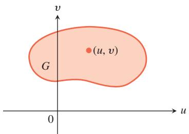
Cartesian uv-plane
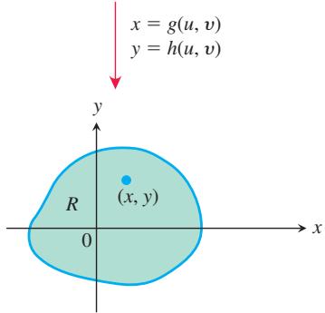
Cartesian xy-plane
FIGURE 14.57 The equations
HISTORICAL BIOGRAPHY Carl Gustav Jacob Jacobi (1804–1851)
Jacobi, one of nineteenth-century Germany’s most accomplished scientists, developed the theory of determinants and transformations into a powerful tool for evaluating multiple integrals and solving differential equations. He also applied transformation methods to study integrals like the ones that arise in the calculation of arc length.
This section introduces the ideas involved in coordinate transformations to evaluate multiple integrals by substitution. The method replaces complicated integrals by ones that are easier to evaluate. Substitutions accomplish this by simplifying the integrand, the limits of integration, or both. A thorough discussion of multivariable transformations and substitutions is best left to a more advanced course, but our introduction here shows how the substitutions just studied reflect the general idea derived for single integral calculus.
To know more, visit the companion Website.
Substitutions in Double Integrals
The polar coordinate substitution of Section 14.4 is a special case of a more general substitution method for double integrals, a method that pictures changes in variables as transformations of regions.
Suppose that a region G in the uv-plane is transformed into the region R in the xy-plane by equations of the form
as suggested in Figure 14.57. We assume the transformation is one-to-one on the interior of
To gain some insight into the question, we look again at the single variable case. To be consistent with how we are using them now, we interchange the variables x and u used in the substitution method for single integrals in Chapter 5, so the equation is
To propose an analogue for substitution in a double integral
Differential Area Change Substituting
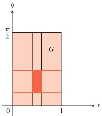
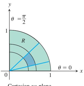
DEFINITION The Jacobian determinant or Jacobian of the coordinate transformation
, 𝑥 = 𝑔 ( 𝑢 , 𝑣 ) is 𝑦 = ℎ ( 𝑢 , 𝑣 ) 𝐽 ( 𝑢 , 𝑣 ) = ∣ 𝜕 𝑥 𝜕 𝑢 𝜕 𝑥 𝜕 𝑣 𝜕 𝑦 𝜕 𝑢 𝜕 𝑦 𝜕 𝑣 ∣ = 𝜕 𝑥 𝜕 𝑢 𝜕 𝑦 𝜕 𝑣 − 𝜕 𝑦 𝜕 𝑢 𝜕 𝑥 𝜕 𝑣 . ( 1 )
The Jacobian can also be denoted by
to help us remember how the determinant in Equation (1) is constructed from the partial derivatives of x and y. The array of partial derivatives in Equation (1) behaves just like the derivative
Now we can answer our original question concerning the relationship of the integral of
THEOREM 3—Substitution for Double Integrals
Suppose that
The derivation of Equation (2) is intricate and properly belongs to a course in advanced calculus, so we do not include it here. We now present examples illustrating the substitution method defined by the equation.
EXAMPLE 1 Find the Jacobian for the polar coordinate transformation
Solution Figure 14.58 shows how the equations
For polar coordinates, we have
Since we assume
This is the same formula we derived independently using a geometric argument for polar area in Section 14.4.
Here is an example of a substitution in which the image of a rectangle under the coordinate transformation is a trapezoid. Transformations like this one are called linear transformations, and their Jacobians are constant throughout G.
EXAMPLE 2 Evaluate
by applying the transformation
and integrating over an appropriate region in the uv-plane.
Solution We sketch the region R of integration in the xy-plane and identify its boundaries (Figure 14.59).
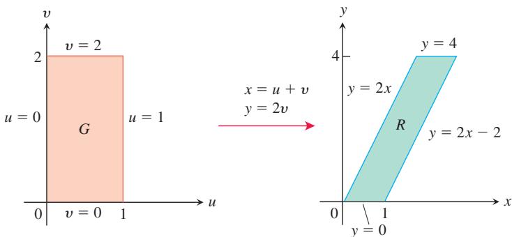
FIGURE 14.59 The equations
To apply Equation (2), we need to find the corresponding uv-region G and the Jacobian of the transformation. To find them, we first solve Equations (4) for x and y in terms of u and v. From those equations it is easy to find algebraically that
We then find the boundaries of G by substituting these expressions into the equations for the boundaries of R (Figure 14.59)
| xy-equations for the boundary of R | Corresponding uv-equations for the boundary of G | Simplified uv-equations |
| x = y/2 | u + v = 2v/2 = v | u = 0 |
| x = (y/2) + 1 | u + v = (2v/2) + 1 = v + 1 | u = 1 |
| y = 0 | 2v = 0 | v = 0 |
| y = 4 | 2v = 4 | v = 2 |
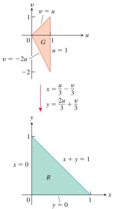
FIGURE 14.60 The equations
From Equations (5) the Jacobian of the transformation is
We now have everything we need to apply Equation (2):
EXAMPLE 3 Evaluate
Solution We sketch the region R of integration in the xy-plane and identify its boundaries (Figure 14.60). The integrand suggests the transformation
From Equations (6), we can find the boundaries of the uv-region G (Figure 14.60).
| xy-equations for the boundary of R | Corresponding uv-equations for the boundary of G | Simplified uv-equations |
| x + y = 1 | u = 1 | |
| x = 0 | v = u | |
| y = 0 | v = -2u |
The Jacobian of the transformation in Equations (6) is
Applying Equation (2), we evaluate the integral:
In the next example we illustrate a nonlinear transformation of coordinates resulting from simplifying the form of the integrand. Like the polar coordinates’ transformation, nonlinear transformations can map a straight-line boundary of a region into a curved boundary (or vice versa with the inverse transformation). In general, nonlinear transformations are more complex to analyze than linear ones, and a complete treatment is left to a more advanced course.
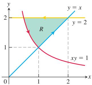
FIGURE 14.61 The region of integration R in Example 4.
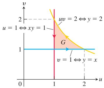
FIGURE 14.62 The boundaries of the region G correspond to those of region R in Figure 14.61. Notice that as we move counterclockwise around the region R, we move counterclockwise around the region G as well. The inverse transformation equations
EXAMPLE 4 Evaluate the integral
Solution The square root terms in the integrand suggest that we might simplify the integration by substituting
with
If G is the region of integration in the uv-plane, then by Equation (2) the transformed double integral under the substitution is
The transformed integrand function is easier to integrate than the original one, so we proceed to determine the limits of integration for the transformed integral.
The region of integration R of the original integral in the xy-plane is shown in Figure 14.61. From the substitution equations
Note the order of integration.
We now evaluate the transformed integral on the right-hand side:
Integrate by parts.
Determinants
Substitutions in Triple Integrals
The cylindrical and spherical coordinate substitutions in Section 14.7 are special cases of a substitution method that pictures changes of variables in triple integrals as transformations of solid regions. The method is like the method for double integrals given by Equation (2) except that now we work in three dimensions instead of two.
Suppose that a solid region
as suggested in Figure 14.63. Then any function
defined on G. If g, h, and k have continuous first partial derivatives, then the integral of
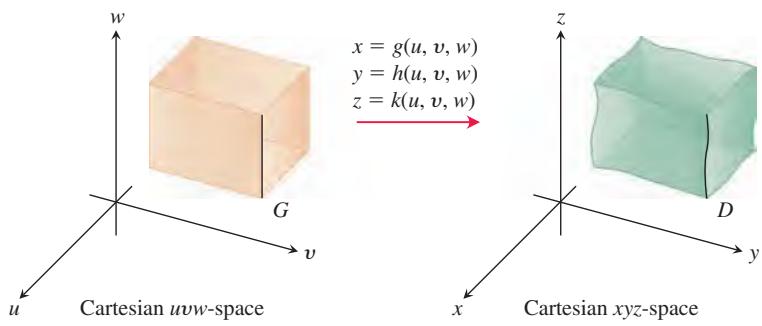
FIGURE 14.63 The equations
The factor
This determinant measures how much the volume near a point in G is being expanded or contracted by the transformation from
For cylindrical coordinates,
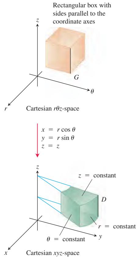
FIGURE 14.64 The equations
(Figure 14.64). The Jacobian of the transformation is
The corresponding version of Equation (7) is
We can drop the absolute value signs because
For spherical coordinates,
(Figure 14.65). The Jacobian of the transformation (see Exercise 23) is
The corresponding version of Equation (7) is
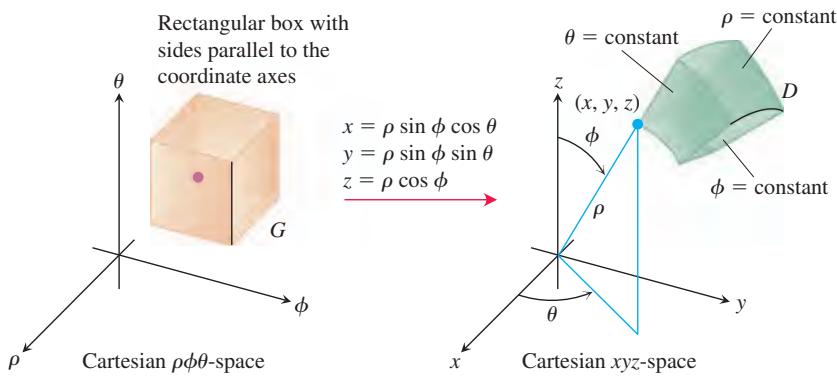
FIGURE 14.65 The equations
We can drop the absolute value signs because
Here is an example of another substitution. Although we could evaluate the integral in this example directly, we have chosen it to illustrate the substitution method in a simple (and fairly intuitive) setting.
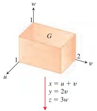
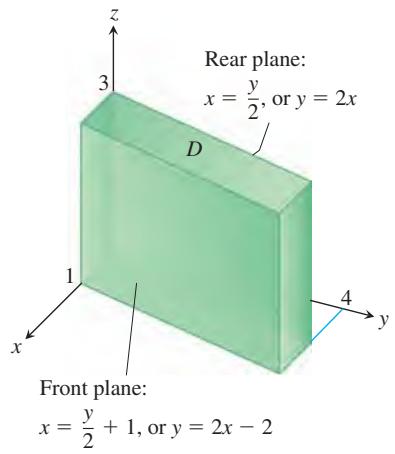
FIGURE 14.66 The equations
EXAMPLE 5 Evaluate
by applying the transformation
and integrating over an appropriate region in uvw-space.
Solution We sketch the solid region D of integration in xyz-space and identify its boundaries (Figure 14.66). In this case, the bounding surfaces are planes.
To apply Equation (7), we need to find the corresponding uvw-region G and the Jacobian of the transformation. To find them, we first solve Equations (8) for x, y, and z in terms of u, v, and w. Routine algebra gives
We then find the boundaries of G by substituting these expressions into the equations for the boundaries of D.
| xyz-equations for the boundary of D | Corresponding uvw-equations for the boundary of G | Simplified uvw-equations |
| x = y/2 | u + v = 2v/2 = v | u = 0 |
| x = (y/2) + 1 | u + v = (2v/2) + 1 = v + 1 | u = 1 |
| y = 0 | 2v = 0 | v = 0 |
| y = 4 | 2v = 4 | v = 2 |
| z = 0 | 3w = 0 | w = 0 |
| z = 3 | 3w = 3 | w = 1 |
The Jacobian of the transformation, again from Equations (9), is
We now have everything we need to apply Equation (7):
Jacobians and Transformed Regions in the Plane
- a. Solve the system
for x and y in terms of u and v. Then find the value of the Jacobian
b. Find the image under the transformation
- a. Solve the system
for x and y in terms of u and v. Then find the value of the Jacobian
b. Find the image under the transformation
- a. Solve the system
for x and y in terms of u and v. Then find the value of the Jacobian
b. Find the image under the transformation
- a. Solve the system
for x and y in terms of u and v. Then find the value of the Jacobian
b. Find the image under the transformation
Substitutions in Double Integrals
- Evaluate the integral
from Example 1 directly by integration with respect to x and y to confirm that its value is 2.
- Use the transformation in Exercise 1 to evaluate the integral
for the region
- Use the transformation in Exercise 3 to evaluate the integral
for the region
- Use the transformation and parallelogram R in Exercise 4 to evaluate the integral
- Let R be the region in the first quadrant of the xy-plane bounded by the hyperbolas xy = 1, xy = 9 and the lines y = x, y = 4x. Use the transformation x = u/v, y = uv with u > 0 and v > 0 to rewrite
as an integral over an appropriate region G in the uv-plane. Then evaluate the uv-integral over G.
- a. Find the Jacobian of the transformation
𝑥 = 𝑢 𝑦 = 𝑢 𝑣 𝐺 : 1 ≤ 𝑢 ≤ 2 1 ≤ 𝑢 𝑣 ≤ 2 𝑢 𝑣
b. Then use Equation (2) to transform the integral
into an integral over G, and evaluate both integrals.
-
Polar moment of inertia of an elliptical plate A thin plate of constant density covers the region bounded by the ellipse
𝑥 2 / 𝑎 2 + 𝑦 2 / 𝑏 2 = 1 𝑥 = 𝑎 𝑟 c o s 𝜃 𝑦 = 𝑏 𝑟 s i n 𝜃 -
The area of an ellipse The area
𝜋 𝑎 𝑏 𝑥 2 / 𝑎 2 + 𝑦 2 / 𝑏 2 = 1 𝑓 ( 𝑥 , 𝑦 ) = 1 𝐺 : 𝑢 2 + 𝑣 2 ≤ 1 -
Use the transformation in Exercise 2 to evaluate the integral
by first writing it as an integral over a region G in the uv-plane.
- Use the transformation
𝑥 = 𝑢 + ( 1 / 2 ) 𝑣 𝑦 = 𝑣
by first writing it as an integral over a region G in the uv-plane.
- Use the transformation
𝑥 = 𝑢 / 𝑣 𝑦 = 𝑢 𝑣
- Use the transformation
𝑥 = 𝑢 2 − 𝑣 2
(Hint: Show that the image of the triangular region G with vertices
Substitutions in Triple Integrals
-
Evaluate the integral in Example 5 by integrating with respect to x, y, and z.
-
Volume of a solid ellipsoid Find the volume of the solid ellipsoid
(Hint: Let
- Evaluate
over the solid ellipsoid D,
(Hint: Let
- Let D be the solid region in xyz-space defined by the inequalities
Evaluate
by applying the transformation
and integrating over an appropriate region G in uvw-space.
Theory and Examples
- Find the Jacobian
𝜕 ( 𝑥 , 𝑦 ) / 𝜕 ( 𝑢 , 𝑣 )
a.
b.
- Find the Jacobian
𝜕 ( 𝑥 , 𝑦 , 𝑧 ) / 𝜕 ( 𝑢 , 𝑣 , 𝑤 )
a.
-
How are double integrals used to calculate areas and average values. Give examples.
-
How can you change a double integral in rectangular coordinates into a double integral in polar coordinates? Why might it be worthwhile to do so? Give an example.
-
Define the triple integral of a function
𝑓 ( 𝑥 , 𝑦 , 𝑧 ) -
How are triple integrals in rectangular coordinates evaluated? How are the limits of integration determined? Give an example.
-
Evaluate the appropriate determinant to show that the Jacobian of the transformation from Cartesian
𝜌 𝜙 𝜃 𝜌 2 s i n 𝜙
CHAPTER 14 Questions to Guide Your Review
-
How are double integrals evaluated as iterated integrals? Does the order of integration matter? How are the limits of integration determined? Give examples.
-
Define the double integral of a function of two variables over a bounded region in the coordinate plane.
-
Substitutions in single integrals How can substitutions in single definite integrals be viewed as transformations of regions? What is the Jacobian in such a case? Illustrate with an example.
-
Centroid of a solid semi-ellipsoid Assuming the result that the centroid of a solid hemisphere lies on the axis of symmetry three-eighths of the way from the base toward the top, show, by transforming the appropriate integrals, that the center of mass of a solid semi-ellipsoid
( 𝑥 2 / 𝑎 2 ) + ( 𝑦 2 / 𝑏 2 ) + ( 𝑧 2 / 𝑐 2 ) ≤ 1 𝑧 ≥ 0 𝑧 -
Cylindrical shells In Section 6.2, we learned how to find the volume of a solid of revolution using the shell method. Specifically, if the region between the curve
𝑦 = 𝑓 ( 𝑥 ) 𝑥 𝑎 𝑏 0 < 𝑎 < 𝑏 𝑦 ∫ 𝑏 𝑎 2 𝜋 𝑥 𝑓 ( 𝑥 ) 𝑑 𝑥 𝑦 𝑧 -
Inverse transform The equations
𝑥 = 𝑔 ( 𝑢 , 𝑣 ) 𝑦 = ℎ ( 𝑢 , 𝑣 ) 𝑢 = 𝛼 ( 𝑥 , 𝑦 ) 𝑣 = 𝛽 ( 𝑥 , 𝑦 )
Equation (10) is proved in advanced calculus. Use it to find the area of the region R in the first quadrant of the xy-plane bounded by the lines y = 2x, 2y = x, and the curves xy = 2, 2xy = 1 for u = xy and v = y/x.
-
(Continuation of Exercise 27.) For the region
𝑅 ∬ 𝑅 𝑦 2 𝑑 𝐴 -
How are double and triple integrals in rectangular coordinates used to calculate volumes, average values, masses, moments, and centers of mass? Give examples.
-
How are triple integrals defined in cylindrical and spherical coordinates? Why might one prefer working in one of these coordinate systems to working in rectangular coordinates?
-
How are triple integrals in cylindrical and spherical coordinates evaluated? How are the limits of integration found? Give examples.
-
How are substitutions in double integrals pictured as transformations of regions in the plane? Give a sample calculation.
-
How are substitutions in triple integrals pictured as transformations of solid regions? Give a sample calculation.
CHAPTER 14 Practice Exercises
Evaluating Double Iterated Integrals
In Exercises 1–4, sketch the region of integration and evaluate the double integral.
-
∫ 1 0 1 ∫ 1 / 𝑦 0 𝑦 𝑒 𝑥 𝑦 𝑑 𝑥 𝑑 𝑦 -
∫ 1 0 ∫ 𝑥 3 0 𝑒 𝑦 / 𝑥 𝑑 𝑦 𝑑 𝑥 -
∫ 3 / 2 0 ∫ √ 9 − 4 𝑡 2 − √ 9 − 4 𝑡 2 𝑡 𝑑 𝑠 𝑑 𝑡 -
∫ 1 0 ∫ 2 − √ 𝑦 √ 𝑦 𝑥 𝑦 𝑑 𝑥 𝑑 𝑦
In Exercises 5–8, sketch the region of integration and write an equivalent integral with the order of integration reversed. Then evaluate both integrals.
5.
-
∫ 1 0 ∫ 𝑥 𝑥 2 √ 𝑥 𝑑 𝑦 𝑑 𝑥 -
∫ 3 / 2 0 ∫ √ 9 − 4 𝑦 2 − √ 9 − 4 𝑦 2 𝑦 𝑑 𝑥 𝑑 𝑦 -
∫ 2 0 ∫ 4 − 𝑥 2 0 2 𝑥 𝑑 𝑦 𝑑 𝑥
Evaluate the integrals in Exercises 9–12.
-
∫ 1 0 ∫ 2 2 𝑦 4 c o s ( 𝑥 2 ) 𝑑 𝑥 𝑑 𝑦 -
∫ 2 0 ∫ 1 𝑦 / 2 𝑒 𝑥 2 𝑑 𝑥 𝑑 𝑦 -
∫ 8 0 ∫ 2 3 √ 𝑥 𝑑 𝑦 𝑑 𝑥 𝑦 4 + 1 -
∫ 1 0 ∫ 1 3 √ 𝑦 2 𝜋 s i n 𝜋 𝑥 2 𝑥 2 𝑑 𝑥 𝑑 𝑦
Areas and Volumes Using Double Integrals
-
Area between line and parabola Find the area of the region enclosed by the line
𝑦 = 2 𝑥 + 4 𝑦 = 4 − 𝑥 2 -
Area bounded by lines and parabola Find the area of the “triangular” region in the xy-plane that is bounded on the right by the parabola
𝑦 = 𝑥 2 𝑥 + 𝑦 = 2 -
Volume of the region under a paraboloid Find the volume under the paraboloid
𝑧 = 𝑥 2 + 𝑦 2 𝑦 = 𝑥 𝑥 = 0 𝑥 + 𝑦 = 2 -
Volume of the region under a parabolic cylinder Find the volume under the parabolic cylinder
𝑧 = 𝑥 2 𝑦 = 6 − 𝑥 2
Average Values
Find the average value of
-
The square bounded by the lines
𝑥 = 1 , 𝑦 = 1 -
The quarter circle
𝑥 2 + 𝑦 2 ≤ 1
Polar Coordinates
Evaluate the integrals in Exercises 19 and 20 by changing to polar coordinates.
-
∫ 1 − 1 ∫ √ 1 − 𝑥 2 − √ 1 − 𝑥 2 2 𝑑 𝑦 𝑑 𝑥 ( 1 + 𝑥 2 + 𝑦 2 ) 2 -
∫ 1 − 1 ∫ √ 1 − 𝑦 2 − √ 1 − 𝑦 2 l n ( 𝑥 2 + 𝑦 2 + 1 ) 𝑑 𝑥 𝑑 𝑦 -
Integrating over a lemniscate Integrate the function
𝑓 ( 𝑥 , 𝑦 ) = 1 / ( 1 + 𝑥 2 + 𝑦 2 ) 2 ( 𝑥 2 + 𝑦 2 ) 2 − ( 𝑥 2 − 𝑦 2 ) = 0 -
Integrate
𝑓 ( 𝑥 , 𝑦 ) = 1 / ( 1 + 𝑥 2 + 𝑦 2 ) 2
a. Triangular region The triangle with vertices
b. First quadrant The first quadrant of the xy-plane.
Evaluating Triple Iterated Integrals
Evaluate the integrals in Exercises 23–26.
23.
-
∫ l n 7 l n 6 ∫ l n 2 0 ∫ l n 5 l n 4 𝑒 ( 𝑥 + 𝑦 + 𝑧 ) 𝑑 𝑧 𝑑 𝑦 𝑑 𝑥 -
∫ 1 0 ∫ 𝑥 2 0 ∫ 𝑥 + 𝑦 0 ( 2 𝑥 − 𝑦 − 𝑧 ) 𝑑 𝑧 𝑑 𝑦 𝑑 𝑥 -
∫ 𝑒 1 ∫ 𝑥 1 ∫ 𝑧 0 2 𝑦 𝑧 3 𝑑 𝑦 𝑑 𝑧 𝑑 𝑥
Volumes and Average Values Using Triple Integrals
- Volume Find the volume of the wedge-shaped solid region enclosed on the side by the cylinder
𝑥 = − c o s 𝑦 − 𝜋 / 2 ≤ 𝑦 ≤ 𝜋 / 2 𝑧 = − 2 𝑥 𝑥 𝑦
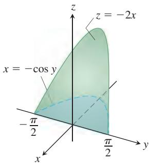
- Volume Find the volume of the solid that is bounded above by the cylinder
𝑧 = 4 − 𝑥 2 𝑥 2 + 𝑦 2 = 4
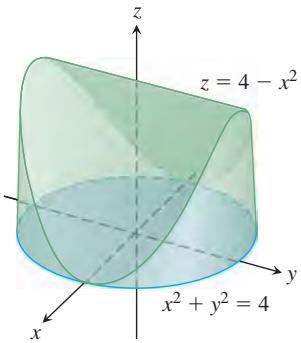
-
Average value Find the average value of
𝑓 ( 𝑥 , 𝑦 , 𝑧 ) = 3 0 𝑥 𝑧 √ 𝑥 2 + 𝑦 -
Average value Find the average value of
𝜌 𝜌 ≤ 𝑎
Cylindrical and Spherical Coordinates
- Cylindrical to rectangular coordinates Convert
to (a) rectangular coordinates with the order of integration dz dx dy and (b) spherical coordinates. Then (c) evaluate one of the integrals.
- Rectangular to cylindrical coordinates (a) Convert to cylindrical coordinates. Then (b) evaluate the new integral.
- Rectangular to spherical coordinates (a) Convert to spherical coordinates. Then (b) evaluate the new integral.
-
Rectangular, cylindrical, and spherical coordinates Write an iterated triple integral for the integral of
𝑓 ( 𝑥 , 𝑦 , 𝑧 ) = 6 + 4 𝑦 𝑧 = √ 𝑥 2 + 𝑦 2 𝑥 2 + 𝑦 2 = 1 -
Cylindrical to rectangular coordinates Set up an integral in rectangular coordinates equivalent to the integral
Arrange the order of integration to be z first, then y, then x.
- Rectangular to cylindrical coordinates The volume of a solid is
a. Describe the solid by giving equations for the surfaces that form its boundary.
b. Convert the integral to cylindrical coordinates, but do not evaluate the integral.
- Spherical versus cylindrical coordinates Triple integrals involving spherical shapes do not always require spherical coordinates for convenient evaluation. Some calculations may be accomplished more easily with cylindrical coordinates. As a case in point, find the volume of the solid region bounded above by the sphere
𝑥 2 + 𝑦 2 + 𝑧 2 = 8
Masses and Moments
-
Finding
𝐼 𝑧 𝛿 = 1 𝜌 = 2 𝜙 = 𝜋 / 3 -
Moment of inertia of a “thick” sphere Find the moment of inertia of a solid of constant density
𝛿 𝑏 ( 𝑎 < 𝑏 ) -
Moment of inertia of an apple Find the moment of inertia about the z-axis of a solid of density
𝛿 = 1 𝜌 = 1 − c o s 𝜙
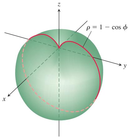
-
Centroid Find the centroid of the “triangular” region bounded by the lines x = 2, y = 2 and the hyperbola xy = 2 in the xy-plane.
-
Centroid Find the centroid of the region between the parabola
𝑥 + 𝑦 2 − 2 𝑦 = 0 𝑥 + 2 𝑦 = 0 -
Polar moment Find the polar moment of inertia about the origin of a thin triangular plate of constant density
𝛿 = 3 -
Polar moment Find the polar moment of inertia about the center of a thin rectangular sheet of constant density
𝛿 = 1
a.
b.
(Hint: Find
-
Inertial moment Find the moment of inertia about the x-axis of a thin plate of constant density
𝛿 ( 0 , 0 ) ( 3 , 0 ) ( 3 , 2 ) -
Plate with variable density Find the center of mass and the moments of inertia about the coordinate axes of a thin plate bounded by the line y = x and the parabola
𝑦 = 𝑥 2 𝛿 ( 𝑥 , 𝑦 ) = 𝑥 + 1 -
Plate with variable density Find the mass and first moments about the coordinate axes of a thin square plate bounded by the lines
𝑥 = ± 1 𝑦 = ± 1 𝑥 𝑦 𝛿 ( 𝑥 , 𝑦 ) = 𝑥 2 + 𝑦 2 + 1 / 3 -
Triangles with same inertial moment Find the moment of inertia about the x-axis of a thin triangular plate of constant density
𝛿 [ 0 , 𝑏 ] -
Centroid Find the centroid of the region in the polar coordinate plane defined by the inequalities
0 ≤ 𝑟 ≤ 3 − 𝜋 / 3 ≤ 𝜃 ≤ 𝜋 / 3 -
Centroid Find the centroid of the region in the first quadrant bounded by the rays
𝜃 = 0 𝜃 = 𝜋 / 2 -
a. Centroid Find the centroid of the region in the polar coordinate plane that lies inside the cardioid
𝑟 = 1 + c o s 𝜃
b. Sketch the region and show the centroid in your sketch.
- a. Centroid Find the centroid of the plane region defined by the polar coordinate inequalities
0 ≤ 𝑟 ≤ 𝑎 , − 𝛼 ≤ 𝜃 ≤ 𝛼 0 < 𝛼 ≤ 𝜋 𝛼 → 𝜋 −
b. Sketch the region for
Substitutions
- Show that if u = x - y and v = y, then for any continuous f,
- What relationship must hold between the constants
𝑎 , 𝑏 𝑐
(Hint: Let
CHAPTER 14 Additional and Advanced Exercises
Volumes
-
Sand pile: double and triple integrals The base of a sand pile covers the region in the xy-plane that is bounded by the parabola
𝑥 2 + 𝑦 = 6 ( 𝑥 , 𝑦 ) 𝑥 2 -
Water in a hemispherical bowl A hemispherical bowl of radius 5 cm is filled with water to within 3 cm of the top. Find the volume of water in the bowl.
-
Solid cylindrical region between two planes Find the volume of the portion of the solid cylinder
𝑥 2 + 𝑦 2 ≤ 1 𝑥 + 𝑦 + 𝑧 = 2 -
Sphere and paraboloid Find the volume of the solid region bounded above by the sphere
𝑥 2 + 𝑦 2 + 𝑧 2 = 2 𝑧 = 𝑥 2 + 𝑦 2 -
Two paraboloids Find the volume of the solid region bounded above by the paraboloid
𝑧 = 3 − 𝑥 2 − 𝑦 2 𝑧 = 2 𝑥 2 + 2 𝑦 2 -
Spherical coordinates Find the volume of the solid region enclosed by the spherical coordinate surface
𝜌 = 2 s i n 𝜙
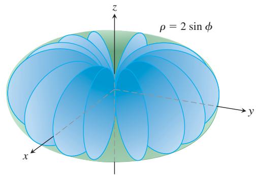
- Hole in solid ball A circular cylindrical hole is bored through a ball, the axis of the hole being a diameter of the sphere. The volume of the remaining solid is
a. Find the radius of the hole and the radius of the sphere.
b. Evaluate the integral.
-
Ball and cylinder Find the volume of material cut from the ball
𝑟 2 + 𝑧 2 ≤ 9 𝑟 = 3 s i n 𝜃 -
Two paraboloids Find the volume of the solid region enclosed by the surfaces
𝑧 = 𝑥 2 + 𝑦 2 𝑧 = ( 𝑥 2 + 𝑦 2 + 1 ) / 2 -
Cylinder and surface z = xy Find the volume of the solid region in the first octant that lies between the cylinders r = 1 and r = 2 and is bounded below by the xy-plane and above by the surface z = xy.
Changing the Order of Integration
- Evaluate the integral
(Hint: Use the relation
to form a double integral, and evaluate the integral by changing the order of integration.)
- a. Polar coordinates Show, by changing to polar coordinates, that
where
b. Rewrite the Cartesian integral with the order of integration reversed.
- Reducing a double to a single integral By changing the order of integration, show that the following double integral can be reduced to a single integral:
Similarly, it can be shown that
- Transforming a double integral to obtain constant limits Sometimes a multiple integral with variable limits can be changed into one with constant limits. By changing the order of integration, show that
Masses and Moments
-
Minimizing polar inertia A thin plate of constant density is to occupy the triangular region in the first quadrant of the xy-plane having vertices
( 0 , 0 ) ( 𝑎 , 0 ) ( 𝑎 , 1 / 𝑎 ) -
Polar inertia of triangular plate Find the polar moment of inertia about the origin of a thin triangular plate of constant density
𝛿 = 3 -
Mass and polar inertia of a counterweight The counterweight of a flywheel of constant density 1 has the form of the smaller segment cut from a circle of radius
𝑎 𝑏 ( 𝑏 < 𝑎 ) -
Centroid of a boomerang Find the centroid of the boomerang-shaped region between the parabolas
𝑦 2 = − 4 ( 𝑥 − 1 ) 𝑦 2 = − 2 ( 𝑥 − 2 )
Theory and Examples
- Evaluate
where
- Show that
over the rectangle
- Suppose that
𝑓 ( 𝑥 , 𝑦 ) 𝑓 ( 𝑥 , 𝑦 ) = 𝐹 ( 𝑥 ) 𝐺 ( 𝑦 ) 𝑅 : 𝑎 ≤ 𝑥 ≤ 𝑏 , 𝑐 ≤ 𝑦 ≤ 𝑑
The argument is that
a. Give reasons for Steps (i) through (iv).
When it applies, Equation (1) can be a time-saver. Use it to evaluate the following integrals.
- Let
𝐷 𝑢 𝑓 𝑓 ( 𝑥 , 𝑦 ) = ( 𝑥 2 + 𝑦 2 ) / 2 𝑢 = 𝑢 1 𝑖 + 𝑢 2 𝑗
a. Finding average value Find the average value of
b. Average value and centroid Show in general that the average value of
- The value of
Γ ( 1 / 2 )
extends the factorial function from the nonnegative integers to other real values. Of particular interest in the theory of differential equations is the number
a. If you have not yet done Exercise 41 in Section 14.4, do it now to show that
b. Substitute
-
Total electrical charge over circular plate The electrical charge distribution on a circular plate of radius R meters is
𝜎 ( 𝑟 , 𝜃 ) = 𝑘 𝑟 ( 1 − s i n 𝜃 ) 2 𝜎 -
A parabolic rain gauge A bowl is in the shape of the graph of
𝑧 = 𝑥 2 + 𝑦 2 -
Water in a satellite dish A parabolic satellite dish is 2 m wide and 1/2 m deep. Its axis of symmetry is tilted 30 degrees from the vertical.
a. Set up, but do not evaluate, a triple integral in rectangular coordinates that gives the amount of water the satellite dish will hold. (Hint: Put your coordinate system so that the satellite dish is in “standard position” and the plane of the water level is slanted.) (Caution: The limits of integration are not “nice.”)
b. What would be the smallest tilt of the satellite dish so that it holds no water?
- An infinite half-cylinder Let D be the interior of the infinite right circular half-cylinder of radius 1 with its single-end face suspended 1 unit above the origin and its axis the ray from
( 0 , 0 , 1 ) ∞
- Hypervolume We have learned that
∫ 𝑏 𝑎 1 𝑑 𝑥 [ 𝑎 , 𝑏 ] ∬ 𝑅 1 𝑑 𝐴 ∭ 𝐷 1 𝑑 𝑉 ∭ 𝑄 1 𝑑 𝑉 𝑥 2 + 𝑦 2 + 𝑧 2 + 𝑤 2 = 1
CHAPTER 14 Technology Application Projects
Mathematica/Maple Projects
Projects can be found within MyLab Math.
-
Take Your Chances: Try the Monte Carlo Technique for Numerical Integration in Three Dimensions Use the Monte Carlo technique to integrate numerically in three dimensions.
-
Means and Moments and Exploring New Plotting Techniques, Part II Use the method of moments in a form that makes use of geometric symmetry as well as multiple integration.