Chapter 8: Techniques of Integration

教材插图

OVERVIEW The Fundamental Theorem tells us how to evaluate a definite integral once we have an antiderivative for the integrand function. However, finding antiderivatives (or indefinite integrals) is not as straightforward as finding derivatives. In this chapter we study a number of important techniques that apply to finding integrals for specialized classes of functions such as trigonometric functions, products of certain functions, and rational functions. Since we cannot always find an antiderivative, we develop numerical methods for calculating definite integrals. We also study integrals for which the domain or range is infinite, called improper integrals.

8.1 Using Basic Integration Formulas

Table 8.1 summarizes the indefinite integrals of many of the functions we have studied so far, and the substitution method helps us use the table to evaluate more complicated functions involving these basic ones. In this section we combine the Substitution Rules (studied in Chapter 5) with algebraic methods and trigonometric identities to help us use Table 8.1. A more extensive Table of Integrals is given at the back of the chapter, and we discuss its use in Section 8.6.

Sometimes we have to rewrite an integral to match it to a standard form of the type displayed in Table 8.1. We start with an example of this procedure.

EXAMPLE 1 Evaluate the integral

\int 53 2 𝑥 - 3 \sqrt 𝑥 2 - 3 𝑥 + 1 𝑑 𝑥 .

Solution We rewrite the integral and apply the Substitution Rule for Definite Integrals presented in Section 5.6, to find

\int 53 2 𝑥 - 3 \sqrt 𝑥 2 - 3 𝑥 + 1 𝑑 𝑥 = \int 111 𝑑 𝑢 \sqrt 𝑢 𝑢 = 𝑥 2 - 3 𝑥 + 1, 𝑑 𝑢 = (2 𝑥 - 3) 𝑑 𝑥; = \int 111 𝑢 - 1 / 2 𝑑 𝑢 = 2 \sqrt 𝑢] 111 = 2 (\sqrt 11 - 1) \approx 4 . 6 3 . (T a b l e 8.1, F o r m u l a 2)

TABLE 8.1 Basic integration formulas

$\int 𝑘 𝑑 𝑥 = 𝑘 𝑥 + 𝐶$ (any number $𝑘$ )
$\int 𝑥 𝑛 𝑑 𝑥 = 𝑥 𝑛 + 1 𝑛 + 1 + 𝐶 (𝑛 \neq - 1)$
$\int 𝑑 𝑥 𝑥 = l n | 𝑥 | + 𝐶$
$\int 𝑒 𝑥 𝑑 𝑥 = 𝑒 𝑥 + 𝐶$
$\int 𝑎 𝑥 𝑑 𝑥 = 𝑎 𝑥 l n 𝑎 + 𝐶 (𝑎 > 0, 𝑎 \neq 1)$
$\int s i n 𝑥 𝑑 𝑥 = - c o s 𝑥 + 𝐶$
$\int c o s 𝑥 𝑑 𝑥 = s i n 𝑥 + 𝐶$
$\int s e c 2 𝑥 𝑑 𝑥 = t a n 𝑥 + 𝐶$
$\int c s c 2 𝑥 𝑑 𝑥 = - c o t 𝑥 + 𝐶$
$\int s e c 𝑥 t a n 𝑥 𝑑 𝑥 = s e c 𝑥 + 𝐶$
$\int c s c 𝑥 c o t 𝑥 𝑑 𝑥 = - c s c 𝑥 + 𝐶$
$\int t a n 𝑥 𝑑 𝑥 = l n | s e c 𝑥 | + 𝐶$
$\int c o t 𝑥 𝑑 𝑥 = l n | s i n 𝑥 | + 𝐶$
$\int s e c 𝑥 𝑑 𝑥 = l n | s e c 𝑥 + t a n 𝑥 | + 𝐶$
$\int c s c 𝑥 𝑑 𝑥 = - l n | c s c 𝑥 + c o t 𝑥 | + 𝐶$
$\int s i n h 𝑥 𝑑 𝑥 = c o s h 𝑥 + 𝐶$
$\int c o s h 𝑥 𝑑 𝑥 = s i n h 𝑥 + 𝐶$
$\int 𝑑 𝑥 \sqrt 𝑎 2 - 𝑥 2 = a r c s i n (𝑥 𝑎) + 𝐶$
$\int 𝑑 𝑥 𝑎 2 + 𝑥 2 = 1 𝑎 a r c t a n (𝑥 𝑎) + 𝐶$
$\int 𝑑 𝑥 𝑥 \sqrt 𝑥 2 - 𝑎 2 = 1 𝑎 a r c s e c ∣ 𝑥 𝑎 ∣ + 𝐶$
$\int 𝑑 𝑥 \sqrt 𝑎 2 + 𝑥 2 = s i n h - 1 (𝑥 𝑎) + 𝐶 (𝑎 > 0)$
$\int 𝑑 𝑥 \sqrt 𝑥 2 - 𝑎 2 = c o s h - 1 (𝑥 𝑎) + 𝐶 (𝑥 > 𝑎 > 0)$

EXAMPLE 2 Complete the square to evaluate

\int 𝑑 𝑥 \sqrt 8 𝑥 - 𝑥 2 .

Solution We complete the square to simplify the denominator:

8 𝑥 - 𝑥 2 = - (𝑥 2 - 8 𝑥) = - (𝑥 2 - 8 𝑥 + 16 - 16) = - (𝑥 2 - 8 𝑥 + 16) + 16 = 16 - (𝑥 - 4) 2 .

Then

\int 𝑑 𝑥 \sqrt 8 𝑥 - 𝑥 2 = \int 𝑑 𝑥 \sqrt 16 - (𝑥 - 4) 2 = \int 𝑑 𝑢 \sqrt 𝑎 2 - 𝑢 2 𝑎 = 4, 𝑢 = (𝑥 - 4), = a r c s i n (𝑢 𝑎) + 𝐶 𝑑 𝑢 = 𝑑 𝑥 = a r c s i n (𝑥 - 4 4) + 𝐶 . (T a b l e 8.1, F o r m u l a 18)

EXAMPLE 3 Evaluate the integral

\int (c o s 𝑥 s i n 2 𝑥 + s i n 𝑥 c o s 2 𝑥) 𝑑 𝑥 .

Solution We can replace the integrand with an equivalent trigonometric expression using the Sine Addition Formula to obtain a simple substitution:

\int (c o s 𝑥 s i n 2 𝑥 + s i n 𝑥 c o s 2 𝑥) 𝑑 𝑥 = \int s i n (𝑥 + 2 𝑥) 𝑑 𝑥 = \int s i n 3 𝑥 𝑑 𝑥 = \int 13 s i n 𝑢 𝑑 𝑢 𝑢 = 3 𝑥, 𝑑 𝑢 = 3 𝑑 𝑥 = - 13 c o s 3 𝑥 + 𝐶 . T a b l e 8.1, F o r m u l a 6

In Section 5.5 we found the indefinite integral of the secant function by multiplying it by a fractional form equal to one, and then integrating the equivalent result. We can use that same procedure in other instances as well, as we illustrate next.

EXAMPLE 4 Find $\int 𝜋 / 4 0 𝑑 𝑥 1 - s i n 𝑥 .$

Solution We multiply the numerator and denominator of the integrand by $1 + s i n 𝑥$ . This procedure transforms the integral into one we can evaluate:

\int 𝜋 / 4 0 𝑑 𝑥 1 - s i n 𝑥 = \int 𝜋 / 4 0 1 1 - s i n 𝑥 \cdot 1 + s i n 𝑥 1 + s i n 𝑥 𝑑 𝑥 M u l t i p l y a n d d i v i d e b y c o n j u g a t e . = \int 𝜋 / 4 0 1 + s i n 𝑥 1 - s i n 2 𝑥 𝑑 𝑥 S i m p l i f y . = \int 𝜋 / 4 0 1 + s i n 𝑥 c o s 2 𝑥 𝑑 𝑥 1 - s i n 2 𝑥 = c o s 2 𝑥 = \int 𝜋 / 4 0 (s e c 2 𝑥 + s e c 𝑥 t a n 𝑥) 𝑑 𝑥 U s e T a b l e 8.1, F o r m u l a s 8 a n d 10 = [t a n 𝑥 + s e c 𝑥] 𝜋 / 4 0 = (1 + \sqrt 2 - (0 + 1)) = \sqrt 2 .

EXAMPLE 5 Evaluate

\int 3 𝑥 2 - 7 𝑥 3 𝑥 + 2 𝑑 𝑥 .

𝑥 - 3 3 𝑥 + 2 ――――――) 3 𝑥 2 - 7 𝑥 3 𝑥 2 + 2 𝑥 - 9 𝑥 - 9 𝑥 - 6 + 6

Solution The integrand is an improper fraction since the degree of the numerator is greater than the degree of the denominator. To integrate it, we perform long division to obtain a quotient plus a remainder that is a proper fraction:

3 𝑥 2 - 7 𝑥 3 𝑥 + 2 = 𝑥 - 3 + 6 3 𝑥 + 2 .

Therefore,

\int 3 𝑥 2 - 7 𝑥 3 𝑥 + 2 𝑑 𝑥 = \int (𝑥 - 3 + 6 3 𝑥 + 2) 𝑑 𝑥 = 𝑥 2 2 - 3 𝑥 + 2 l n | 3 𝑥 + 2 | + 𝐶 .

Reducing an improper fraction by long division (Example 5) does not always lead to an expression we can integrate directly. We see what to do about that in Section 8.5.

EXAMPLE 6 Evaluate

\int 3 𝑥 + 2 \sqrt 1 - 𝑥 2 𝑑 𝑥 .

Solution We first separate the integrand to get

\int 3 𝑥 + 2 \sqrt 1 - 𝑥 2 𝑑 𝑥 = 3 \int 𝑥 𝑑 𝑥 \sqrt 1 - 𝑥 2 + 2 \int 𝑑 𝑥 \sqrt 1 - 𝑥 2 .

In the first of these new integrals, we substitute

𝑢 = 1 - 𝑥 2, 𝑑 𝑢 = - 2 𝑥 𝑑 𝑥, s o 𝑥 𝑑 𝑥 = - 12 𝑑 𝑢 .

Then we obtain

3 \int 𝑥 𝑑 𝑥 \sqrt 1 - 𝑥 2 = 3 \int (- 1 / 2) 𝑑 𝑢 \sqrt 𝑢 = - 32 \int 𝑢 - 1 / 2 𝑑 𝑢 = - 32 \cdot 𝑢 1 / 2 1 / 2 + 𝐶 1 = - 3 \sqrt 1 - 𝑥 2 + 𝐶 1 .

The second of the new integrals is a standard form,

2 \int 𝑑 𝑥 \sqrt 1 - 𝑥 2 = 2 a r c s i n 𝑥 + 𝐶 2 . T a b l e 8.1, F o r m u l a 18

Combining these results and renaming $𝐶 1 + 𝐶 2$ as C gives

\int 3 𝑥 + 2 \sqrt 1 - 𝑥 2 𝑑 𝑥 = - 3 \sqrt 1 - 𝑥 2 + 2 a r c s i n 𝑥 + 𝐶 .

The question of what to substitute for in an integrand is not always quite so clear. Sometimes we simply proceed by trial-and-error, and if nothing works out, we then try another method altogether. The next several sections of the text present some of these new methods, but substitution works in the following example.

EXAMPLE 7 Evaluate

\int 𝑑 𝑥 (1 + \sqrt 𝑥) 3 .

Solution We might try substituting for the term $\sqrt 𝑥$ , but the derivative factor $1 / \sqrt 𝑥$ is missing from the integrand, so this substitution will not help. The other possibility is to substitute for $(1 + \sqrt 𝑥)$ , and it turns out this works:

\int 𝑑 𝑥 (1 + \sqrt 𝑥) 3 = \int 2 (𝑢 - 1) 𝑑 𝑢 𝑢 3 𝑢 = 1 + \sqrt 𝑥, 𝑑 𝑢 = 1 2 \sqrt 𝑥 𝑑 𝑥; 𝑑 𝑥 = 2 \sqrt 𝑥 𝑑 𝑢 = 2 (𝑢 - 1) 𝑑 𝑢 = \int (2 𝑢 2 - 2 𝑢 3) 𝑑 𝑢

= - 2 𝑢 + 1 𝑢 2 + 𝐶

= 1 - 2 𝑢 𝑢 2 + 𝐶

= 1 - 2 (1 + \sqrt 𝑥) (1 + \sqrt 𝑥) 2 + 𝐶

= 𝐶 - 1 + 2 \sqrt 𝑥 (1 + \sqrt 𝑥) 2 .

When evaluating definite integrals, a property of the integrand may help us in calculating the result.

EXAMPLE 8 Evaluate

\int 𝜋 / 2 - 𝜋 / 2 𝑥 3 c o s 𝑥 𝑑 𝑥 .

Solution No substitution or algebraic manipulation is clearly helpful here. But we observe that the interval of integration is the symmetric interval $[- 𝜋 / 2, 𝜋 / 2]$ . Moreover, the factor $𝑥 3$ is an odd function, and $c o s 𝑥$ is an even function, so their product is odd. Therefore,

$\int 𝜋 / 2 - 𝜋 / 2 𝑥 3 c o s 𝑥 𝑑 𝑥 = 0 .$ Theorem 8, Section 5.6

EXERCISES 8.1

Assorted Integrations

The integrals in Exercises 1–44 are in no particular order. Evaluate each integral using any algebraic method, trigonometric identity, or substitution you think is appropriate.

$\int 10 16 𝑥 8 𝑥 2 + 2 𝑑 𝑥$
$\int 𝑥 2 𝑥 2 + 1 𝑑 𝑥$
$\int (s e c 𝑥 - t a n 𝑥) 2 𝑑 𝑥$
$\int 𝜋 / 3 𝜋 / 4 𝑑 𝑥 c o s 2 𝑥 t a n 𝑥$
$\int 1 - 𝑥 \sqrt 1 - 𝑥 2 𝑑 𝑥$
$\int 𝑑 𝑥 𝑥 - \sqrt 𝑥$
$\int 𝑒 - c o t 𝑧 s i n 2 𝑧 𝑑 𝑧$
$\int 2 l n 𝑧 3 16 𝑧 𝑑 𝑧$
$\int 𝑑 𝑧 𝑒 𝑧 + 𝑒 - 𝑧$
$\int 21 8 𝑑 𝑥 𝑥 2 - 2 𝑥 + 2$
$\int 0 - 1 4 𝑑 𝑥 1 + (2 𝑥 + 1) 2$
$\int 3 - 1 4 𝑥 2 - 7 2 𝑥 + 3 𝑑 𝑥$
$\int 𝑑 𝑡 1 - s e c 𝑡$
$\int c s c 𝑡 s i n 3 𝑡 𝑑 𝑡$
$\int 𝜋 / 4 0 1 + s i n 𝜃 c o s 2 𝜃 𝑑 𝜃$
$\int 𝑑 𝜃 \sqrt 2 𝜃 - 𝜃 2$
$\int l n 𝑦 𝑦 + 4 𝑦 l n 2 𝑦 𝑑 𝑦$
$\int 2 \sqrt 𝑦 𝑑 𝑦 2 \sqrt 𝑦$
$\int 𝑑 𝜃 s e c 𝜃 + t a n 𝜃$
$\int 𝑑 𝑡 𝑡 \sqrt 3 + 𝑡 2$
$\int 4 𝑡 3 - 𝑡 2 + 16 𝑡 𝑡 2 + 4 𝑑 𝑡$
$\int 𝑥 + 2 \sqrt 𝑥 - 1 2 𝑥 \sqrt 𝑥 - 1 𝑑 𝑥$
$\int 𝜋 / 2 0 \sqrt 1 - c o s 𝜃 𝑑 𝜃$
$\int (s e c 𝑡 + c o t 𝑡) 2 𝑑 𝑡$
$\int 𝑑 𝑦 \sqrt 𝑒 2 𝑦 - 1$
$\int 6 𝑑 𝑦 \sqrt 𝑦 (1 + 𝑦)$
$\int 2 𝑑 𝑥 𝑥 \sqrt 1 - 4 l n 2 𝑥$
$\int 𝑑 𝑥 (𝑥 - 2) \sqrt 𝑥 2 - 4 𝑥 + 3$
$\int (c s c 𝑥 - s e c 𝑥) (s i n 𝑥 + c o s 𝑥) 𝑑 𝑥$
$\int 3 s i n h (𝑥 2 + l n 5) 𝑑 𝑥$
$\int 3 \sqrt 2 2 𝑥 3 𝑥 2 - 1 𝑑 𝑥$
$\int 1 - 1 \sqrt 1 + 𝑥 2 s i n 𝑥 𝑑 𝑥$
$\int 0 - 1 \sqrt 1 + 𝑦 1 - 𝑦 𝑑 𝑦$
$\int 𝑒 𝑧 + 𝑒 𝑧 𝑑 𝑧$
$\int 7 𝑑 𝑥 (𝑥 - 1) \sqrt 𝑥 2 - 2 𝑥 - 48$
$\int 𝑑 𝑥 (2 𝑥 + 1) \sqrt 4 𝑥 + 4 𝑥 2$
$\int 2 𝜃 3 - 7 𝜃 2 + 7 𝜃 2 𝜃 - 5 𝑑 𝜃$
$\int 𝑑 𝜃 c o s 𝜃 - 1$
$\int 𝑑 𝑥 1 + 𝑒 𝑥$
$\int \sqrt 𝑥 1 + 𝑥 3 𝑑 𝑥$

Hint: Use long division.

H i n t : L e t 𝑢 = 𝑥 3 / 2 .

$\int 𝑒 3 𝑥 𝑒 𝑥 + 1 𝑑 𝑥$
$\int 2 𝑥 - 1 3 𝑥 𝑑 𝑥$
$\int 1 \sqrt 𝑥 (1 + 𝑥) 𝑑 𝑥$
$\int t a n 𝜃 + 3 s i n 𝜃 𝑑 𝜃$

Theory and Examples

Area Find the area of the region bounded above by $𝑦 = 2 c o s 𝑥$ and below by $𝑦 = s e c 𝑥, - 𝜋 / 4 \leq 𝑥 \leq 𝜋 / 4$ .
Volume Find the volume of the solid generated by revolving the region in Exercise 45 about the x-axis.
Arc length Find the length of the curve $𝑦 = l n (c o s 𝑥)$ , $0 \leq 𝑥 \leq 𝜋 / 3$ .
Arc length Find the length of the curve $𝑦 = l n (s e c 𝑥)$ , $0 \leq 𝑥 \leq 𝜋 / 4$ .
Centroid Find the centroid of the region bounded by the $𝑥$ -axis, the curve $𝑦 = s e c 𝑥$ , and the lines $𝑥 = - 𝜋 / 4$ , $𝑥 = 𝜋 / 4$ .
Centroid Find the centroid of the region bounded by the $𝑥$ -axis, the curve $𝑦 = c s c 𝑥$ , and the lines $𝑥 = 𝜋 / 6$ , $𝑥 = 5 𝜋 / 6$ .
The functions $𝑦 = 𝑒 𝑥 3$ and $𝑦 = 𝑥 3 𝑒 𝑥 3$ do not have elementary antiderivatives, but $𝑦 = (1 + 3 𝑥 3) 𝑒 𝑥 3$ does. Evaluate

\int (1 + 3 𝑥 3) 𝑒 𝑥 3 𝑑 𝑥 . 52 . $ 𝑈 𝑠 𝑒 𝑡 ℎ 𝑒 𝑠 𝑢 𝑏 𝑠 𝑡 𝑖 𝑡 𝑢 𝑡 𝑖 𝑜 𝑛 $ 𝑢 = t a n 𝑥 $ 𝑡 𝑜 𝑒 𝑣 𝑎 𝑙 𝑢 𝑎 𝑡 𝑒 𝑡 ℎ 𝑒 𝑖 𝑛 𝑡 𝑒 𝑔 𝑟 𝑎 𝑙 $ \int 𝑑 𝑥 1 + s i n 2 𝑥 . 53 . $ 𝑈 𝑠 𝑒 𝑡 ℎ 𝑒 𝑠 𝑢 𝑏 𝑠 𝑡 𝑖 𝑡 𝑢 𝑡 𝑖 𝑜 𝑛 $ 𝑢 = 𝑥 4 + 1 $ 𝑡 𝑜 𝑒 𝑣 𝑎 𝑙 𝑢 𝑎 𝑡 𝑒 𝑡 ℎ 𝑒 𝑖 𝑛 𝑡 𝑒 𝑔 𝑟 𝑎 𝑙 $ \int 𝑥 7 \sqrt 𝑥 4 + 1 𝑑 𝑥 . 54 . $ 𝑈 𝑠 𝑖 𝑛 𝑔 𝑑 𝑖 𝑓 𝑓 𝑒 𝑟 𝑒 𝑛 𝑡 𝑠 𝑢 𝑏 𝑠 𝑡 𝑖 𝑡 𝑢 𝑡 𝑖 𝑜 𝑛 𝑠 𝑆 ℎ 𝑜 𝑤 𝑡 ℎ 𝑎 𝑡 𝑡 ℎ 𝑒 𝑖 𝑛 𝑡 𝑒 𝑔 𝑟 𝑎 𝑙 $ \int ((𝑥 2 - 1) (𝑥 + 1)) - 2 / 3 𝑑 𝑥

can be evaluated with any of the following substitutions.

a. $𝑢 = 1 / (𝑥 + 1)$

b. $𝑢 = ((𝑥 - 1) / (𝑥 + 1)) 𝑘$ for k = 1, 1/2, 1/3, -1/3, -2/3, and -1

c. $𝑢 = a r c t a n 𝑥$

d. $𝑢 = t a n - 1 \sqrt 𝑥$

e. $𝑢 = t a n - 1 ((𝑥 - 1) / 2)$

f. $𝑢 = a r c c o s 𝑥$

g. $𝑢 = c o s h - 1 𝑥$

8.2 Integration by Parts

What is the value of the integral?

Integration by parts is a technique for simplifying integrals of the form

\int 𝑢 (𝑥) 𝑣' (𝑥) 𝑑 𝑥 .

It is useful when $𝑢$ can be differentiated repeatedly and $𝑣'$ can be integrated repeatedly without difficulty. The integrals

\int 𝑥 c o s 𝑥 𝑑 𝑥 a n d \int 𝑥 2 𝑒 𝑥 𝑑 𝑥

are such integrals because $𝑢 (𝑥) = 𝑥$ or $𝑢 (𝑥) = 𝑥 2$ can be differentiated repeatedly, and $𝑣' (𝑥) = c o s 𝑥$ or $𝑣' (𝑥) = 𝑒 𝑥$ can be integrated repeatedly without difficulty. Integration by parts also applies to integrals like

\int l n 𝑥 𝑑 𝑥 a n d \int 𝑒 𝑥 c o s 𝑥 𝑑 𝑥 .

In the first case, the integrand $l n 𝑥$ can be rewritten as $(l n 𝑥) (1)$ , and $𝑢 (𝑥) = l n 𝑥$ is easy to differentiate while $𝑣' (𝑥) = 1$ easily integrates to x. In the second case, each part of the integrand appears again after repeated differentiation or integration.

Product Rule in Integral Form

If $𝑢$ and $𝑣$ are differentiable functions of $𝑥$ , the Product Rule says that

𝑑 𝑑 𝑥 [𝑢 (𝑥) 𝑣 (𝑥)] = 𝑢' (𝑥) 𝑣 (𝑥) + 𝑢 (𝑥) 𝑣' (𝑥) .

In terms of indefinite integrals, this equation becomes

\int 𝑑 𝑑 𝑥 [𝑢 (𝑥) 𝑣 (𝑥)] 𝑑 𝑥 = \int [𝑢' (𝑥) 𝑣 (𝑥) + 𝑢 (𝑥) 𝑣' (𝑥)] 𝑑 𝑥

\int 𝑑 𝑑 𝑥 [𝑢 (𝑥) 𝑣 (𝑥)] 𝑑 𝑥 = \int 𝑢' (𝑥) 𝑣 (𝑥) 𝑑 𝑥 + \int 𝑢 (𝑥) 𝑣' (𝑥) 𝑑 𝑥 .

Rearranging the terms of this last equation, we get

\int 𝑢 (𝑥) 𝑣' (𝑥) 𝑑 𝑥 = \int 𝑑 𝑑 𝑥 [𝑢 (𝑥) 𝑣 (𝑥)] 𝑑 𝑥 - \int 𝑣 (𝑥) 𝑢' (𝑥) 𝑑 𝑥,

leading to the following integration by parts formula.

Integration by Parts Formula

\int 𝑢 (𝑥) 𝑣' (𝑥) 𝑑 𝑥 = 𝑢 (𝑥) 𝑣 (𝑥) - \int 𝑣 (𝑥) 𝑢' (𝑥) 𝑑 𝑥 (1)

This formula allows us to exchange the problem of computing the integral $\int 𝑢 (𝑥) 𝑣' (𝑥) 𝑑 𝑥$ for the problem of computing a different integral, $\int 𝑣 (𝑥) 𝑢' (𝑥) 𝑑 𝑥$ . In many cases, we can choose the functions u and v so that the second integral is easier to compute than the first. There can be many choices for u and v, and it is not always clear which choice works best, so sometimes we need to try several.

The formula is often given in differential form. With $𝑣' (𝑥) 𝑑 𝑥 = 𝑑 𝜈$ and $𝑢' (𝑥) 𝑑 𝑥 = 𝑑 𝑢$ , the integration by parts formula becomes

Integration by Parts Formula—Differential Version

\int 𝑢 𝑑 𝑣 = 𝑢 𝑣 - \int 𝑣 𝑑 𝑢 (2)

The next examples illustrate the technique.

EXAMPLE 1 Find

\int 𝑥 c o s 𝑥 𝑑 𝑥 .

Solution There is no obvious antiderivative of $𝑥 c o s 𝑥$ , so we use the integration by parts formula

\int 𝑢 (𝑥) 𝑣' (𝑥) 𝑑 𝑥 = 𝑢 (𝑥) 𝑣 (𝑥) - \int 𝑣 (𝑥) 𝑢' (𝑥) 𝑑 𝑥

to change this expression to one that is easier to integrate. We first decide how to choose the functions $𝑢 (𝑥)$ and $𝑣 (𝑥)$ . There is more than one way to do this, but here we choose to factor the expression $𝑥 c o s 𝑥$ into

𝑢 (𝑥) = 𝑥 a n d 𝑣' (𝑥) = c o s 𝑥 .

Next we differentiate $𝑢 (𝑥)$ and find an antiderivative of $𝑣' (𝑥)$ ,

𝑢' (𝑥) = 1 a n d 𝑣 (𝑥) = s i n 𝑥 .

When finding an antiderivative for $𝑣' (𝑥)$ , we have a choice of how to pick a constant of integration C. We choose the constant C = 0, since that makes this antiderivative as simple as possible. We now apply the integration by parts formula:

\int 𝑢 (𝑥) 𝑥 c o s 𝑥 𝑑 𝑥 = 𝑥 s i n 𝑥 - \int 𝑣 (𝑥) s i n 𝑥 (1) 𝑑 𝑥 I n t e g r a t i o n b y p a r t s f o r m u l a = 𝑥 s i n 𝑥 + c o s 𝑥 + 𝐶 I n t e g r a t e a n d s i m p l i f y .

and we have found the integral of the original function.

There are at least four apparent choices available for $𝑢 (𝑥)$ and $𝑣' (𝑥)$ in Example 1:

𝟏 . 𝐋 𝐞 𝐭 𝑢 (𝑥) = 1 a n d 𝑣' (𝑥) = 𝑥 c o s 𝑥 . 𝟐 . 𝐋 𝐞 𝐭 𝑢 (𝑥) = 𝑥 a n d 𝑣' (𝑥) = c o s 𝑥 . 𝟑 . 𝐋 𝐞 𝐭 𝑢 (𝑥) = 𝑥 c o s 𝑥 a n d 𝑣' (𝑥) = 1 . 𝟒 . 𝐋 𝐞 𝐭 𝑢 (𝑥) = c o s 𝑥 a n d 𝑣' (𝑥) = 𝑥 .

We used choice 2 in Example 1. The other three choices lead to integrals that we do not know how to evaluate. For instance, Choice 3, with $𝑢' (𝑥) = c o s 𝑥 - 𝑥 s i n 𝑥$ , leads to the integral

\int (𝑥 c o s 𝑥 - 𝑥 2 s i n 𝑥) 𝑑 𝑥 .

The goal of integration by parts is to go from an integral $\int 𝑢 (𝑥) 𝑣' (𝑥) 𝑑 𝑥$ that we don’t see how to evaluate to an integral $\int 𝑣 (𝑥) 𝑢' (𝑥) 𝑑 𝑥$ that we can evaluate. Generally, we choose $𝑣' (𝑥)$ first to be as much of the integrand as we can readily integrate; then we let $𝑢 (𝑥)$ be the leftover part. When finding $𝑣 (𝑥)$ from $𝑣' (𝑥)$ , any antiderivative will work, and we usually pick the simplest one. In particular, no arbitrary constant of integration is needed in $𝑣 (𝑥)$ because it would simply cancel out of the right-hand side of Equation (2).

* * E X A M P L E 2 * * F i n d \int l n 𝑥 𝑑 𝑥 .

Solution We have not yet seen how to find an antiderivative for $l n 𝑥$ . If we set $𝑢 (𝑥) = l n 𝑥$ , then $𝑢' (𝑥)$ is the simpler function 1/x. It may not appear that a second function $𝑣' (𝑥)$ is multiplying $𝑢 (𝑥) = l n 𝑥$ , but we can choose $𝑣' (𝑥)$ to be the constant function $𝑣' (𝑥) = 1$ . We use the integration by parts formula given in Equation (1), with

𝑢 (𝑥) = l n 𝑥 a n d 𝑣' (𝑥) = 1 .

We differentiate $𝑢 (𝑥)$ and find an antiderivative of $𝑣' (𝑥)$ ,

𝑢' (𝑥) = 1 𝑥 a n d 𝑣 (𝑥) = 𝑥 .

Then

\int l n 𝑥 \cdot 1 𝑑 𝑥 = (l n 𝑥) 𝑥 - \int 𝑥 1 𝑥 𝑑 𝑥 𝑢 (𝑥) 𝑣' (𝑥) = 𝑢 (𝑥) 𝑣 (𝑥) 𝑣 (𝑥) 𝑢' (𝑥) = 𝑥 l n 𝑥 - \int 1 𝑑 𝑥 = 𝑥 l n 𝑥 - 𝑥 + 𝐶 I n t e g r a t i o n b y p a r t s f o r m u l a S i m p l i f y a n d i n t e g r a t e .

In the following examples we use the differential form to indicate the process of integration by parts. The computations are the same, with du and dv providing shorter expressions for $𝑢' (𝑥)$ dx and $𝑣' (𝑥)$ dx.

Sometimes we have to use integration by parts more than once, as in the next example.

EXAMPLE 3 Evaluate

\int 𝑥 2 𝑒 𝑥 𝑑 𝑥 .

Solution We use the integration by parts formula given in Equation (1), with

𝑢 (𝑥) = 𝑥 2 a n d 𝑣' (𝑥) = 𝑒 𝑥 .

We differentiate $𝑢 (𝑥)$ and find an antiderivative of $𝑣' (𝑥)$ ,

𝑢' (𝑥) = 2 𝑥 a n d 𝑣 (𝑥) = 𝑒 𝑥 .

We summarize this choice by setting $𝑑 𝑢 = 𝑢' (𝑥) 𝑑 𝑥$ and $𝑑 𝑣 = 𝑣' (𝑥) 𝑑 𝑥$ , so

𝑑 𝑢 = 2 𝑥 𝑑 𝑥 a n d 𝑑 𝑣 = 𝑒 𝑥 𝑑 𝑥 .

We then have

\int 𝑢 𝑥 2 𝑒 𝑥 𝑑 𝑥 ⏟ 𝑑 𝑣 = 𝑥 2 𝑢 𝑒 𝑥 - \int 𝑣 𝑒 𝑥 2 𝑥 𝑑 𝑥 ⏟ 𝑑 𝑢 = 𝑥 2 𝑒 𝑥 - 2 \int 𝑥 𝑒 𝑥 𝑑 𝑥 I n t e g r a t i o n b y p a r t s f o r m u l a

The new integral is less complicated than the original because the exponent on x is reduced by one. To evaluate the integral on the right, we integrate by parts again with u = x, $𝑑 𝑣 = 𝑒 𝑥 𝑑 𝑥$ . Then du = dx, $𝑣 = 𝑒 𝑥$ , and

\int 𝑥 𝑒 𝑥 𝑑 𝑥 ⏟ 𝑢 𝑑 𝑣 = 𝑥 𝑒 𝑥 ⏟ 𝑢 𝑣 - \int 𝑒 𝑥 𝑑 𝑥 ⏟ 𝑣 𝑑 𝑢 = 𝑥 𝑒 𝑥 - 𝑒 𝑥 + 𝐶 . I n t e g r a t i o n b y p a r t s E q u a t i o n (2) 𝑢 = 𝑥, 𝑑 𝑣 = 𝑒 𝑥 𝑑 𝑥 𝑣 = 𝑒 𝑥, 𝑑 𝑢 = 𝑑 𝑥

Using this last evaluation, we then obtain

\int 𝑥 2 𝑒 𝑥 𝑑 𝑥 = 𝑥 2 𝑒 𝑥 - 2 \int 𝑥 𝑒 𝑥 𝑑 𝑥 = 𝑥 2 𝑒 𝑥 - 2 𝑥 𝑒 𝑥 + 2 𝑒 𝑥 + 𝐶,

where the constant of integration is renamed after substituting for the integral on the right.

The technique of Example 3 works for any integral $\int 𝑥 𝑛 𝑒 𝑥 𝑑 𝑥$ in which $𝑛$ is a positive integer, because differentiating $𝑥 𝑛$ will eventually lead to a constant, and repeatedly integrating $𝑒 𝑥$ is easy.

Integrals like the one in the next example occur in electrical engineering. Their evaluation requires two integrations by parts, followed by solving for the unknown integral.

EXAMPLE 4 Evaluate

\int 𝑒 𝑥 c o s 𝑥 𝑑 𝑥 .

Solution Let $𝑢 = 𝑒 𝑥$ and dv = cos x dx. Then du = $𝑒 𝑥$ dx, v = sin x, and

\int 𝑒 𝑥 c o s 𝑥 𝑑 𝑥 = 𝑒 𝑥 s i n 𝑥 - \int 𝑒 𝑥 s i n 𝑥 𝑑 𝑥 .

The second integral is like the first except that it has $s i n 𝑥$ in place of $c o s 𝑥$ . To evaluate it, we use integration by parts with

𝑢 = 𝑒 𝑥, 𝑑 𝑣 = s i n 𝑥 𝑑 𝑥, 𝑣 = - c o s 𝑥, 𝑑 𝑢 = 𝑒 𝑥 𝑑 𝑥 .

Then

\int 𝑒 𝑥 c o s 𝑥 𝑑 𝑥 = 𝑒 𝑥 s i n 𝑥 - (- 𝑒 𝑥 c o s 𝑥 - \int (- c o s 𝑥) (𝑒 𝑥 𝑑 𝑥)) = 𝑒 𝑥 s i n 𝑥 + 𝑒 𝑥 c o s 𝑥 - \int 𝑒 𝑥 c o s 𝑥 𝑑 𝑥 .

The unknown integral now appears on both sides of the equation, but with opposite signs. Adding the integral to both sides and adding the constant of integration gives

2 \int 𝑒 𝑥 c o s 𝑥 𝑑 𝑥 = 𝑒 𝑥 s i n 𝑥 + 𝑒 𝑥 c o s 𝑥 + 𝐶 1 .

Dividing by 2 and renaming the constant of integration then gives

\int 𝑒 𝑥 c o s 𝑥 𝑑 𝑥 = 𝑒 𝑥 s i n 𝑥 + 𝑒 𝑥 c o s 𝑥 2 + 𝐶 .

EXAMPLE 5 Obtain a formula that expresses the integral

\int c o s 𝑛 𝑥 𝑑 𝑥

in terms of an integral of a lower power of $c o s 𝑥$ .

Solution We may think of $c o s 𝑛 𝑥$ as $c o s 𝑛 - 1 𝑥 \cdot c o s 𝑥$ . Then we let

𝑢 = c o s 𝑛 - 1 𝑥 a n d 𝑑 𝑣 = c o s 𝑥 𝑑 𝑥,

so that

𝑑 𝑢 = (𝑛 - 1) (c o s 𝑛 - 2 𝑥) (- s i n 𝑥 𝑑 𝑥) a n d 𝑣 = s i n 𝑥 .

Integration by parts then gives

\int c o s 𝑛 𝑥 𝑑 𝑥 = c o s 𝑛 - 1 𝑥 s i n 𝑥 + (𝑛 - 1) \int s i n 2 𝑥 c o s 𝑛 - 2 𝑥 𝑑 𝑥 = c o s 𝑛 - 1 𝑥 s i n 𝑥 + (𝑛 - 1) \int (1 - c o s 2 𝑥) c o s 𝑛 - 2 𝑥 𝑑 𝑥 = c o s 𝑛 - 1 𝑥 s i n 𝑥 + (𝑛 - 1) \int c o s 𝑛 - 2 𝑥 𝑑 𝑥 - (𝑛 - 1) \int c o s 𝑛 𝑥 𝑑 𝑥 .

If we add

(𝑛 - 1) \int c o s 𝑛 𝑥 𝑑 𝑥

to both sides of this equation, we obtain

𝑛 \int c o s 𝑛 𝑥 𝑑 𝑥 = c o s 𝑛 - 1 𝑥 s i n 𝑥 + (𝑛 - 1) \int c o s 𝑛 - 2 𝑥 𝑑 𝑥 .

We then divide through by $𝑛$ , and the final result is

\int c o s 𝑛 𝑥 𝑑 𝑥 = c o s 𝑛 - 1 𝑥 s i n 𝑥 𝑛 + 𝑛 - 1 𝑛 \int c o s 𝑛 - 2 𝑥 𝑑 𝑥 .

The formula found in Example 5 is called a reduction formula because it replaces an integral containing some power of a function with an integral of the same form having the power reduced. When n is a positive integer, we may apply the formula repeatedly until the remaining integral is easy to evaluate. For example, the result in Example 5 tells us that

\int c o s 3 𝑥 𝑑 𝑥 = c o s 2 𝑥 s i n 𝑥 3 + 23 \int c o s 𝑥 𝑑 𝑥 = 13 c o s 2 𝑥 s i n 𝑥 + 23 s i n 𝑥 + 𝐶 .

Evaluating Definite Integrals by Parts

The integration by parts formula in Equation (1) can be combined with Part 2 of the Fundamental Theorem in order to evaluate definite integrals by parts. Assuming that both $𝑢'$ and $𝑣'$ are continuous over the interval $[𝑎, 𝑏]$ , Part 2 of the Fundamental Theorem gives

Integration by Parts Formula for Definite Integrals

\int 𝑏 𝑎 𝑢 (𝑥) 𝑣' (𝑥) 𝑑 𝑥 = 𝑢 (𝑥) 𝑣 (𝑥)] 𝑏 𝑎 - \int 𝑏 𝑎 𝑣 (𝑥) 𝑢' (𝑥) 𝑑 𝑥 (3)

教材插图

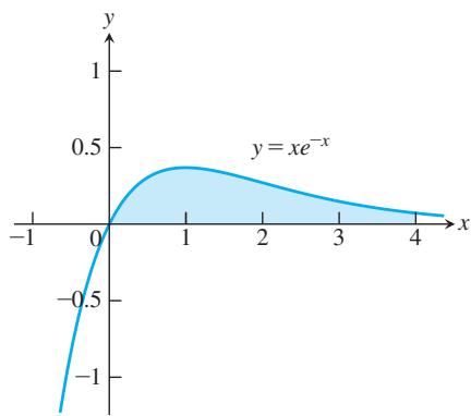
FIGURE 8.1 The region in Example 6.

EXAMPLE 6 Find the area of the region bounded by the curve $𝑦 = 𝑥 𝑒 - 𝑥$ and the $𝑥$ -axis from $𝑥 = 0$ to $𝑥 = 4$ .

Solution The region is shaded in Figure 8.1. Its area is

\int 40 𝑥 𝑒 - 𝑥 𝑑 𝑥 .

Let $𝑢 = 𝑥$ , $𝑑 𝑣 = 𝑒 - 𝑥 𝑑 𝑥$ , $𝑣 = - 𝑒 - 𝑥$ , and $𝑑 𝑢 = 𝑑 𝑥$ . Then

$\int 40 𝑥 𝑒 - 𝑥 𝑑 𝑥 = - 𝑥 𝑒 - 𝑥 ∣ 40 - \int 40 (- 𝑒 - 𝑥) 𝑑 𝑥$ Integration by parts Formula (3) $= [- 4 𝑒 - 4 - (- 0 𝑒 - 0)] + \int 40 𝑒 - 𝑥 𝑑 𝑥$ $= - 4 𝑒 - 4 - 𝑒 - 𝑥 ∣ 40$ $= - 4 𝑒 - 4 - (𝑒 - 4 - 𝑒 - 0) = 1 - 5 𝑒 - 4 \approx 0.91 .$

EXERCISES 8.2

Integration by Parts

Evaluate the integrals in Exercises 1–24 using integration by parts.

$\int 𝑥 s i n 𝑥 2 𝑑 𝑥$
$\int 𝜃 c o s 𝜋 𝜃 𝑑 𝜃$
$\int 𝑡 2 c o s 𝑡 𝑑 𝑡$
$\int 𝑥 2 s i n 𝑥 𝑑 𝑥$
$\int 21 𝑥 l n 𝑥 𝑑 𝑥$
$\int 𝑒 1 𝑥 3 l n 𝑥 𝑑 𝑥$
$\int 𝑥 𝑒 𝑥 𝑑 𝑥$
$\int 𝑥 𝑒 3 𝑥 𝑑 𝑥$
$\int 𝑥 2 𝑒 - 𝑥 𝑑 𝑥$
$\int (𝑥 2 - 2 𝑥 + 1) 𝑒 2 𝑥 𝑑 𝑥$
$\int t a n - 1 𝑦 𝑑 𝑦$
$\int a r c s i n 𝑦 𝑑 𝑦$
$\int 𝑥 s e c 2 𝑥 𝑑 𝑥$
$\int 4 𝑥 s e c 2 2 𝑥 𝑑 𝑥$
$\int 𝑥 3 𝑒 𝑥 𝑑 𝑥$
$\int 𝑝 4 𝑒 - 𝑝 𝑑 𝑝$
$\int (𝑥 2 - 5 𝑥) 𝑒 𝑥 𝑑 𝑥$
$\int (𝑟 2 + 𝑟 + 1) 𝑒 𝑟 𝑑 𝑟$

\int \sqrt 𝑥 l n 𝑥 𝑑 𝑥

$\int 𝑥 5 𝑒 𝑥 𝑑 𝑥$
$\int 𝑡 2 𝑒 4 𝑡 𝑑 𝑡$
$\int 𝑒 𝜃 s i n 𝜃 𝑑 𝜃$
$\int 𝑒 - 𝑦 c o s 𝑦 𝑑 𝑦$
$\int 𝑒 2 𝑥 c o s 3 𝑥 𝑑 𝑥$
$\int 𝑒 - 2 𝑥 s i n 2 𝑥 𝑑 𝑥$

Using Substitution

Evaluate the integrals in Exercises 25–30 by using a substitution prior to integration by parts.

$\int 𝑒 \sqrt 3 𝑠 + 9 𝑑 𝑠$
$\int 10 𝑥 \sqrt 1 - 𝑥 𝑑 𝑥$
$\int 𝜋 / 3 0 𝑥 t a n 2 𝑥 𝑑 𝑥$
$\int l n (𝑥 + 𝑥 2) 𝑑 𝑥$
$\int s i n (l n 𝑥) 𝑑 𝑥$
$\int 𝑧 (l n 𝑧) 2 𝑑 𝑧$

Evaluating Integrals

Evaluate the integrals in Exercises 31–56. Some integrals do not require integration by parts.

$\int 𝑥 s e c 𝑥 2 𝑑 𝑥$
$\int c o s \sqrt 𝑥 \sqrt 𝑥 𝑑 𝑥$
$\int 𝑥 (l n 𝑥) 2 𝑑 𝑥$
$\int 1 𝑥 (l n 𝑥) 2 𝑑 𝑥$
$\int l n 𝑥 𝑥 2 𝑑 𝑥$
$\int (l n 𝑥) 3 𝑥 𝑑 𝑥$
$\int 𝑥 3 𝑒 𝑥 4 𝑑 𝑥$
$\int 𝑥 5 𝑒 𝑥 3 𝑑 𝑥$
$\int 𝑥 3 \sqrt 𝑥 2 + 1 𝑑 𝑥$
$\int 𝑥 2 s i n 𝑥 3 𝑑 𝑥$
$\int s i n 3 𝑥 c o s 2 𝑥 𝑑 𝑥$
$\int s i n 2 𝑥 c o s 4 𝑥 𝑑 𝑥$
$\int 𝑒 \sqrt 𝑥 \sqrt 𝑥 𝑑 𝑥$
$\int c o s \sqrt 𝑥 𝑑 𝑥$
$\int \sqrt 𝑥 𝑒 \sqrt 𝑥 𝑑 𝑥$
$\int 𝜋 / 2 0 𝜃 2 s i n 2 𝜃 𝑑 𝜃$
$\int 𝜋 / 2 0 𝑥 3 c o s 2 𝑥 𝑑 𝑥$
$\int 2 2 / \sqrt 3 𝑡 s e c - 1 𝑡 𝑑 𝑡$
$\int 1 / \sqrt 2 0 2 𝑥 a r c s i n (𝑥 2) 𝑑 𝑥$
$\int 𝑥 a r c t a n 𝑥 𝑑 𝑥$
$\int 𝑥 2 t a n - 1 𝑥 2 𝑑 𝑥$
$\int (1 + 2 𝑥 2) 𝑒 𝑥 2 𝑑 𝑥$
$\int 𝑥 𝑒 𝑥 (𝑥 + 1) 2 𝑑 𝑥$
$\int \sqrt 𝑥 (a r c s i n \sqrt 𝑥) 𝑑 𝑥$
$\int (s i n - 1 𝑥) 2 \sqrt 1 - 𝑥 2 𝑑 𝑥$

Theory and Examples

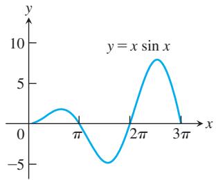
Finding area Find the area of the region enclosed by the curve $𝑦 = 𝑥 s i n 𝑥$ and the x-axis (see the accompanying figure) for

a. $0 \leq 𝑥 \leq 𝜋 .$

b. $𝜋 \leq 𝑥 \leq 2 𝜋 .$

c. $2 𝜋 \leq 𝑥 \leq 3 𝜋 .$

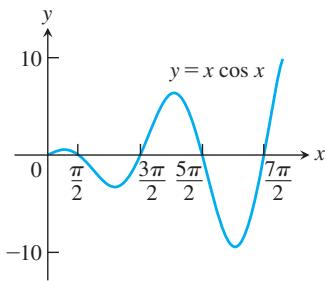
d. What pattern do you see here? What is the area between the curve and the x-axis for $𝑛 𝜋 \leq 𝑥 \leq (𝑛 + 1) 𝜋$ , n an arbitrary nonnegative integer? Give reasons for your answer.

教材插图

Finding area Find the area of the region enclosed by the curve $𝑦 = 𝑥 c o s 𝑥$ and the x-axis (see the accompanying figure) for

a. $𝜋 / 2 \leq 𝑥 \leq 3 𝜋 / 2 .$

b. $3 𝜋 / 2 \leq 𝑥 \leq 5 𝜋 / 2$ .

c. $5 𝜋 / 2 \leq 𝑥 \leq 7 𝜋 / 2 .$

d. What pattern do you see? What is the area between the curve and the x-axis for

(2 𝑛 - 1 2) 𝜋 \leq 𝑥 \leq (2 𝑛 + 1 2) 𝜋,

n an arbitrary positive integer? Give reasons for your answer.

教材插图

Finding volume Find the volume of the solid generated by revolving the region in the first quadrant bounded by the coordinate axes, the curve $𝑦 = 𝑒 𝑥$ , and the line $𝑥 = l n 2$ about the line $𝑥 = l n 2$ .
Finding volume Find the volume of the solid generated by revolving the region in the first quadrant bounded by the coordinate axes, the curve $𝑦 = 𝑒 - 𝑥$ , and the line x = 1

a. about the y-axis.

b. about the line x = 1.

Finding volume Find the volume of the solid generated by revolving the region in the first quadrant bounded by the coordinate axes and the curve $𝑦 = c o s 𝑥$ , $0 \leq 𝑥 \leq 𝜋 / 2$ , about

a. the y-axis.

b. the line $𝑥 = 𝜋 / 2$ .

Finding volume Find the volume of the solid generated by revolving the region bounded by the x-axis and the curve $𝑦 = 𝑥 s i n 𝑥, 0 \leq 𝑥 \leq 𝜋$ , about

a. the y-axis.

b. the line $𝑥 = 𝜋$ .

(See Exercise 57 for a graph.)

Consider the region bounded by the graphs of $𝑦 = l n 𝑥$ , $𝑦 = 0$ , and $𝑥 = 𝑒$ .

a. Find the area of the region.

b. Find the volume of the solid formed by revolving this region about the x-axis.

c. Find the volume of the solid formed by revolving this region about the line x = -2.

d. Find the centroid of the region.

Consider the region bounded by the graphs of $𝑦 = a r c t a n 𝑥$ , $𝑦 = 0$ , and $𝑥 = 1$ .

a. Find the area of the region.

b. Find the volume of the solid formed by revolving this region about the y-axis.

Average value A retarding force, symbolized by the dashpot in the accompanying figure, slows the motion of the weighted spring so that the mass’s position at time $𝑡$ is

𝑦 = 2 𝑒 - 𝑡 c o s 𝑡, 𝑡 \geq 0 .

Find the average value of $𝑦$ over the interval $0 \leq 𝑡 \leq 2 𝜋$ .

教材插图

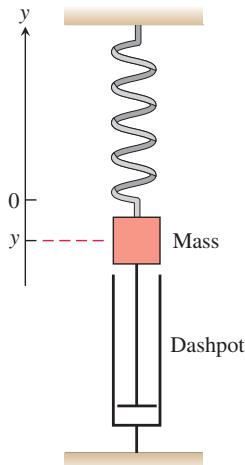
Average value In a mass-spring-dashpot system like the one in Exercise 65, the mass’s position at time $𝑡$ is

𝑦 = 4 𝑒 - 𝑡 (s i n 𝑡 - c o s 𝑡), 𝑡 \geq 0 .

Find the average value of $𝑦$ over the interval $0 \leq 𝑡 \leq 2 𝜋$ .

Reduction Formulas

In Exercises 67–73, use integration by parts to establish the reduction formula.

$\int 𝑥 𝑛 c o s 𝑥 𝑑 𝑥 = 𝑥 𝑛 s i n 𝑥 - 𝑛 \int 𝑥 𝑛 - 1 s i n 𝑥 𝑑 𝑥$
$\int 𝑥 𝑛 s i n 𝑥 𝑑 𝑥 = - 𝑥 𝑛 c o s 𝑥 + 𝑛 \int 𝑥 𝑛 - 1 c o s 𝑥 𝑑 𝑥$
$\int 𝑥 𝑛 𝑒 𝑎 𝑥 𝑑 𝑥 = 𝑥 𝑛 𝑒 𝑎 𝑥 𝑎 - 𝑛 𝑎 \int 𝑥 𝑛 - 1 𝑒 𝑎 𝑥 𝑑 𝑥, 𝑎 \neq 0$
$\int (l n 𝑥) 𝑛 𝑑 𝑥 = 𝑥 (l n 𝑥) 𝑛 - 𝑛 \int (l n 𝑥) 𝑛 - 1 𝑑 𝑥$

71 . \int 𝑥 𝑚 (l n 𝑥) 𝑛 𝑑 𝑥 = 𝑥 𝑚 + 1 𝑚 + 1 (l n 𝑥) 𝑛 - 𝑛 𝑚 + 1 \int 𝑥 𝑚 (l n 𝑥) 𝑛 - 1 𝑑 𝑥, 𝑚 \neq - 1

72 . \int 𝑥 𝑛 \sqrt 𝑥 + 1 𝑑 𝑥 = 2 𝑥 𝑛 2 𝑛 + 3 (𝑥 + 1) 3 / 2 - 2 𝑛 2 𝑛 + 3 \int 𝑥 𝑛 - 1 \sqrt 𝑥 + 1 𝑑 𝑥

73 . \int 𝑥 𝑛 \sqrt 𝑥 + 1 𝑑 𝑥 = 2 𝑥 𝑛 2 𝑛 + 1 \sqrt 𝑥 + 1 - 2 𝑛 2 𝑛 + 1 \int 𝑥 𝑛 - 1 \sqrt 𝑥 + 1 𝑑 𝑥 74 . $ 𝑈 𝑠 𝑒 𝐸 𝑥 𝑎 𝑚 𝑝 𝑙 𝑒 5 𝑡 𝑜 𝑠 ℎ 𝑜 𝑤 𝑡 ℎ 𝑎 𝑡 $ \int 𝜋 / 2 0 s i n 𝑛 𝑥 𝑑 𝑥 = \int 𝜋 / 2 0 c o s 𝑛 𝑥 𝑑 𝑥 = ⎧ { {⎨ { {⎩ (𝜋 2) 1 \cdot 3 \cdot 5 \dots (𝑛 - 1) 2 \cdot 4 \cdot 6 \dots 𝑛, 𝑛 e v e n 2 \cdot 4 \cdot 6 \dots (𝑛 - 1) 1 \cdot 3 \cdot 5 \dots 𝑛, 𝑛 o d d 75 . $ 𝑆 ℎ 𝑜 𝑤 𝑡 ℎ 𝑎 𝑡 $ \int 𝑏 𝑎 (\int 𝑏 𝑥 𝑓 (𝑡) 𝑑 𝑡) 𝑑 𝑥 = \int 𝑏 𝑎 (𝑥 - 𝑎) 𝑓 (𝑥) 𝑑 𝑥 . 76 . $ 𝑈 𝑠 𝑒 𝑖 𝑛 𝑡 𝑒 𝑔 𝑟 𝑎 𝑡 𝑖 𝑜 𝑛 𝑏 𝑦 𝑝 𝑎 𝑟 𝑡 𝑠 𝑡 𝑜 𝑜 𝑏 𝑡 𝑎 𝑖 𝑛 𝑡 ℎ 𝑒 𝑓 𝑜 𝑟 𝑚 𝑢 𝑙 𝑎 $ \int \sqrt 1 - 𝑥 2 𝑑 𝑥 = 12 𝑥 \sqrt 1 - 𝑥 2 + 12 \int 1 \sqrt 1 - 𝑥 2 𝑑 𝑥 .

Integrating Inverses of Functions

Integration by parts leads to a rule for integrating inverses that usually gives good results:

\int 𝑓 - 1 (𝑥) 𝑑 𝑥 = \int 𝑦 𝑓' (𝑦) 𝑑 𝑦 𝑦 = 𝑓 - 1 (𝑥), 𝑥 = 𝑓 (𝑦) 𝑑 𝑥 = 𝑓' (𝑦) 𝑑 𝑦 = 𝑦 𝑓 (𝑦) - \int 𝑓 (𝑦) 𝑑 𝑦 I n t e g r a t i o n b y p a r t s w i t h 𝑢 = 𝑦, 𝑑 𝑣 = 𝑓' (𝑦) 𝑑 𝑦 = 𝑥 𝑓 - 1 (𝑥) - \int 𝑓 (𝑦) 𝑑 𝑦

The idea is to take the most complicated part of the integral, in this case $𝑓 - 1 (𝑥)$ , and simplify it first. For the integral of $l n 𝑥$ , we get

\int l n 𝑥 𝑑 𝑥 = \int 𝑦 𝑒 𝑦 𝑑 𝑦 𝑦 = l n 𝑥, 𝑥 = 𝑒 𝑦 𝑑 𝑥 = 𝑒 𝑦 𝑑 𝑦 = 𝑦 𝑒 𝑦 - 𝑒 𝑦 + 𝐶 = 𝑥 l n 𝑥 - 𝑥 + 𝐶 .

For the integral of $a r c c o s 𝑥$ , we get

\int a r c c o s 𝑥 𝑑 𝑥 = 𝑥 a r c c o s 𝑥 - \int c o s 𝑦 𝑑 𝑦 = 𝑥 a r c c o s 𝑥 - s i n 𝑦 + 𝐶 = 𝑥 a r c c o s 𝑥 - s i n (a r c c o s 𝑥) + 𝐶 . 𝑦 = a r c c o s 𝑥

Use the formula

\int 𝑓 - 1 (𝑥) 𝑑 𝑥 = 𝑥 𝑓 - 1 (𝑥) - \int 𝑓 (𝑦) 𝑑 𝑦 𝑦 = 𝑓 - 1 (𝑥) (4)

to evaluate the integrals in Exercises 77–80. Express your answers in terms of x.

$\int a r c s e c 𝑥 𝑑 𝑥$
$\int a r c t a n 𝑥 𝑑 𝑥$
$\int s e c - 1 𝑥 𝑑 𝑥$
$\int l o g 2 𝑥 𝑑 𝑥$

Another way to integrate $𝑓 - 1 (𝑥)$ (when $𝑓 - 1$ is integrable) is to use integration by parts with $𝑢 = 𝑓 - 1 (𝑥)$ and dv = dx to rewrite the integral of $𝑓 - 1$ as

\int 𝑓 - 1 (𝑥) 𝑑 𝑥 = 𝑥 𝑓 - 1 (𝑥) - \int 𝑥 (𝑑 𝑑 𝑥 𝑓 - 1 (𝑥)) 𝑑 𝑥 . (5)

Exercises 81 and 82 compare the results of using Equations (4) and (5).

Equations (4) and (5) give different formulas for the integral of $a r c c o s 𝑥$ :

𝐚 . \int a r c c o s 𝑥 𝑑 𝑥 = 𝑥 a r c c o s 𝑥 - s i n (a r c c o s 𝑥) + 𝐶 (E q . (4)

\int a r c c o s 𝑥 𝑑 𝑥 = 𝑥 a r c c o s 𝑥 - \sqrt 1 - 𝑥 2 + 𝐶 (E q . (5)

Can both integrations be correct? Explain.

Equations (4) and (5) lead to different formulas for the integral of $a r c t a n 𝑥$ :

𝐚 . \int a r c t a n 𝑥 𝑑 𝑥 = 𝑥 a r c t a n 𝑥 - l n s e c (a r c t a n 𝑥) + 𝐶 (E q . (4)

\int a r c t a n 𝑥 𝑑 𝑥 = 𝑥 a r c t a n 𝑥 - l n \sqrt 1 + 𝑥 2 + 𝐶 (E q . (5)

Can both integrations be correct? Explain.

Evaluate the integrals in Exercises 83 and 84 with (a) Eq. (4) and (b) Eq. (5). In each case, check your work by differentiating your answer with respect to x.

83 . \int s i n h - 1 𝑥 𝑑 𝑥 84 . \int t a n h - 1 𝑥 𝑑 𝑥

8.3 Trigonometric Integrals

Trigonometric integrals involve algebraic combinations of the six basic trigonometric functions. In principle, we can always express such integrals in terms of sines and cosines, but it is often simpler to work with other functions, as in the integral

\int s e c 2 𝑥 𝑑 𝑥 = t a n 𝑥 + 𝐶 .

The general idea is to use identities to transform the integrals we must find into integrals that are easier to work with.

Products of Powers of Sines and Cosines

We begin with integrals of the form

\int s i n 𝑚 𝑥 c o s 𝑛 𝑥 𝑑 𝑥,

where m and n are nonnegative integers (positive or zero). We can divide the appropriate substitution into three cases according to m and n being odd or even.

Case 1 If $𝑚$ is odd in $\int s i n 𝑚 𝑥 c o s 𝑛 𝑥 𝑑 𝑥$ , we write $𝑚$ as $2 𝑘 + 1$ and use the identity $s i n 2 𝑥 = 1 - c o s 2 𝑥$ to obtain

s i n 𝑚 𝑥 = s i n 2 𝑘 + 1 𝑥 = (s i n 2 𝑥) 𝑘 s i n 𝑥 = (1 - c o s 2 𝑥) 𝑘 s i n 𝑥 . (1)

Then we substitute $𝑢 = c o s 𝑥$ and $𝑑 𝑢 = - s i n 𝑥 𝑑 𝑥$ .

Case 2 If $𝑛$ is odd in $\int s i n 𝑚 𝑥 c o s 𝑛 𝑥 𝑑 𝑥$ , we write $𝑛$ as $2 𝑘 + 1$ and use the identity $c o s 2 𝑥 = 1 - s i n 2 𝑥$ to obtain

c o s 𝑛 𝑥 = c o s 2 𝑘 + 1 𝑥 = (c o s 2 𝑥) 𝑘 c o s 𝑥 = (1 - s i n 2 𝑥) 𝑘 c o s 𝑥 .

We then substitute $𝑢 = s i n 𝑥$ and $𝑑 𝑢 = c o s 𝑥 𝑑 𝑥$ .

Case 3 If both m and n are even in $\int s i n 𝑚 𝑥 c o s 𝑛 𝑥 𝑑 𝑥$ , we substitute

s i n 2 𝑥 = 1 - c o s 2 𝑥 2, c o s 2 𝑥 = 1 + c o s 2 𝑥 2 (2)

to reduce the integrand to one in lower powers of $c o s 2 𝑥$ .

Here are some examples illustrating each case.

EXAMPLE 1 Evaluate $\int s i n 3 𝑥 c o s 2 𝑥 𝑑 𝑥$ .

Solution This is an example of Case 1.

\int s i n 3 𝑥 c o s 2 𝑥 𝑑 𝑥 = \int s i n 2 𝑥 c o s 2 𝑥 s i n 𝑥 𝑑 𝑥 𝑚 i s o d d . = \int (1 - c o s 2 𝑥) (c o s 2 𝑥) s i n 𝑥 𝑑 𝑥 s i n 2 𝑥 = 1 - c o s 2 𝑥 = \int (1 - 𝑢 2) (𝑢 2) (- 𝑑 𝑢) 𝑢 = c o s 𝑥, 𝑑 𝑢 = - s i n 𝑥 𝑑 𝑥 = \int (𝑢 4 - 𝑢 2) 𝑑 𝑢 D i s t r i b u t e . = 𝑢 5 5 - 𝑢 3 3 + 𝐶 = c o s 5 𝑥 5 - c o s 3 𝑥 3 + 𝐶 ◼

EXAMPLE 2 Evaluate

\int c o s 5 𝑥 𝑑 𝑥 .

Solution This is an example of Case 2, where m = 0 is even and n = 5 is odd.

\int c o s 5 𝑥 𝑑 𝑥 = \int c o s 4 𝑥 c o s 𝑥 𝑑 𝑥 = \int (1 - s i n 2 𝑥) 2 c o s 𝑥 𝑑 𝑥 = \int (1 - 𝑢 2) 2 𝑑 𝑢 𝑢 = s i n 𝑥, 𝑑 𝑢 = c o s 𝑥 𝑑 𝑥 = \int (1 - 2 𝑢 2 + 𝑢 4) 𝑑 𝑢 S q u a r e 1 - 𝑢 2 . = 𝑢 - 23 𝑢 3 + 15 𝑢 5 + 𝐶 = s i n 𝑥 - 23 s i n 3 𝑥 + 15 s i n 5 𝑥 + 𝐶

EXAMPLE 3 Evaluate

\int s i n 2 𝑥 c o s 4 𝑥 𝑑 𝑥 .

Solution This is an example of Case 3.

\int s i n 2 𝑥 c o s 4 𝑥 𝑑 𝑥 = \int (1 - c o s 2 𝑥 2) (1 + c o s 2 𝑥 2) 2 𝑑 𝑥 𝑚 a n d 𝑛 b o t h e v e n = 18 \int (1 - c o s 2 𝑥) (1 + 2 c o s 2 𝑥 + c o s 2 2 𝑥) 𝑑 𝑥 = 18 \int (1 + c o s 2 𝑥 - c o s 2 2 𝑥 - c o s 3 2 𝑥) 𝑑 𝑥 = 18 [𝑥 + 12 s i n 2 𝑥 - \int (c o s 2 2 𝑥 + c o s 3 2 𝑥) 𝑑 𝑥]

For the term involving $c o s 2 2 𝑥$ , we use

\int c o s 2 2 𝑥 𝑑 𝑥 = 12 \int (1 + c o s 4 𝑥) 𝑑 𝑥 U s e t h e i d e n t i t y c o s 2 𝜃 = (1 + c o s 2 𝜃) / 2, w i t h 𝜃 = 2 𝑥 . = 12 (𝑥 + 14 s i n 4 𝑥) + 𝐶 1 .

For the $c o s 3 2 𝑥$ term, we have

\int c o s 3 2 𝑥 𝑑 𝑥 = \int (1 - s i n 2 2 𝑥) c o s 2 𝑥 𝑑 𝑥 = 12 \int (1 - 𝑢 2) 𝑑 𝑢 = 12 (s i n 2 𝑥 - 13 s i n 3 2 𝑥) + 𝐶 2 .

Combining everything and simplifying, we get

\int s i n 2 𝑥 c o s 4 𝑥 𝑑 𝑥 = 116 (𝑥 - 14 s i n 4 𝑥 + 13 s i n 3 2 𝑥) + 𝐶 .

Eliminating Square Roots

In the next example, we use the identity $c o s 2 𝜃 = (1 + c o s 2 𝜃) / 2$ to eliminate a square root.

EXAMPLE 4 Evaluate

\int 𝜋 / 4 0 \sqrt 1 + c o s 4 𝑥 𝑑 𝑥 .

Solution To eliminate the square root, we use the identity

c o s 2 𝜃 = 1 + c o s 2 𝜃 2 o r 1 + c o s 2 𝜃 = 2 c o s 2 𝜃 .

With $𝜃 = 2 𝑥$ , this becomes

1 + c o s 4 𝑥 = 2 c o s 2 2 𝑥 .

Therefore,

\int 𝜋 / 4 0 \sqrt 1 + c o s 4 𝑥 𝑑 𝑥 = \int 𝜋 / 4 0 \sqrt 2 c o s 2 2 𝑥 𝑑 𝑥 = \int 𝜋 / 4 0 \sqrt 2 \sqrt c o s 2 2 𝑥 𝑑 𝑥 = \sqrt 2 \int 𝜋 / 4 0 | c o s 2 𝑥 | 𝑑 𝑥 = \sqrt 2 \int 𝜋 / 4 0 c o s 2 𝑥 𝑑 𝑥 o n [0, 𝜋 / 4] = \sqrt 2 [s i n 2 𝑥 2] 𝜋 / 4 0 = \sqrt 2 2 [1 - 0] = \sqrt 2 2 .

Integrals of Powers of tan x and sec x

We know how to integrate the tangent and secant functions and their squares. To integrate higher powers, we use the identities $t a n 2 𝑥 = s e c 2 𝑥 - 1$ and $s e c 2 𝑥 = t a n 2 𝑥 + 1$ , and integrate by parts when necessary to reduce the higher powers to lower powers.

EXAMPLE 5 Evaluate

\int t a n 4 𝑥 𝑑 𝑥 .

Solution

\int t a n 4 𝑥 𝑑 𝑥 = \int t a n 2 𝑥 \cdot t a n 2 𝑥 𝑑 𝑥 = \int t a n 2 𝑥 \cdot (s e c 2 𝑥 - 1) 𝑑 𝑥 t a n 2 𝑥 = s e c 2 𝑥 - 1 = \int t a n 2 𝑥 s e c 2 𝑥 𝑑 𝑥 - \int t a n 2 𝑥 𝑑 𝑥 = \int t a n 2 𝑥 s e c 2 𝑥 𝑑 𝑥 - \int (s e c 2 𝑥 - 1) 𝑑 𝑥 t a n 2 𝑥 = s e c 2 𝑥 - 1 = \int t a n 2 𝑥 s e c 2 𝑥 𝑑 𝑥 - \int s e c 2 𝑥 𝑑 𝑥 + \int 𝑑 𝑥

In the first integral, we let

𝑢 = t a n 𝑥, 𝑑 𝑢 = s e c 2 𝑥 𝑑 𝑥

and have

\int 𝑢 2 𝑑 𝑢 = 13 𝑢 3 + 𝐶 1 .

The remaining integrals are standard forms, so

\int t a n 4 𝑥 𝑑 𝑥 = 13 t a n 3 𝑥 - t a n 𝑥 + 𝑥 + 𝐶 .

EXAMPLE 6 Evaluate

\int s e c 3 𝑥 𝑑 𝑥 .

Solution We integrate by parts using

𝑢 = s e c 𝑥, 𝑑 𝑣 = s e c 2 𝑥 𝑑 𝑥, 𝑣 = t a n 𝑥, 𝑑 𝑢 = s e c 𝑥 t a n 𝑥 𝑑 𝑥 .

Then

\int s e c 3 𝑥 𝑑 𝑥 = s e c 𝑥 t a n 𝑥 - \int (t a n 𝑥) (s e c 𝑥 t a n 𝑥) 𝑑 𝑥 = s e c 𝑥 t a n 𝑥 - \int (s e c 2 𝑥 - 1) s e c 𝑥 𝑑 𝑥 = s e c 𝑥 t a n 𝑥 - \int s e c 3 𝑥 𝑑 𝑥 + \int s e c 𝑥 𝑑 𝑥 I n t e g r a t e b y p a r t s . t a n 2 𝑥 = s e c 2 𝑥 - 1

Combining the two secant-cubed integrals gives

2 \int s e c 3 𝑥 𝑑 𝑥 = s e c 𝑥 t a n 𝑥 + \int s e c 𝑥 𝑑 𝑥

and therefore

\int s e c 3 𝑥 𝑑 𝑥 = 12 s e c 𝑥 t a n 𝑥 + 12 l n | s e c 𝑥 + t a n 𝑥 | + 𝐶 .

EXAMPLE 7 Evaluate

\int t a n 4 𝑥 s e c 4 𝑥 𝑑 𝑥 .

Solution

\int (t a n 4 𝑥) (s e c 4 𝑥) 𝑑 𝑥 = \int (t a n 4 𝑥) (1 + t a n 2 𝑥) (s e c 2 𝑥) 𝑑 𝑥 s e c 2 𝑥 = 1 + t a n 2 𝑥 = \int (t a n 4 𝑥 + t a n 6 𝑥) (s e c 2 𝑥) 𝑑 𝑥 D i s t r i b u t e . = \int (𝑢 4 + 𝑢 6) 𝑑 𝑢 = 𝑢 5 5 + 𝑢 7 7 + 𝐶 𝑢 = t a n 𝑥, = t a n 5 𝑥 5 + t a n 7 𝑥 7 + 𝐶 𝑑 𝑢 = s e c 2 𝑥 𝑑 𝑥

Products of Sines and Cosines

The integrals

\int s i n 𝑚 𝑥 s i n 𝑛 𝑥 𝑑 𝑥, \int s i n 𝑚 𝑥 c o s 𝑛 𝑥 𝑑 𝑥, a n d \int c o s 𝑚 𝑥 c o s 𝑛 𝑥 𝑑 𝑥

arise in many applications involving periodic functions. We can evaluate these integrals through integration by parts, but two such integrations are required in each case. It is simpler to use the following identities.

s i n 𝑚 𝑥 s i n 𝑛 𝑥 = 12 [c o s (𝑚 - 𝑛) 𝑥 - c o s (𝑚 + 𝑛) 𝑥] (3)

s i n 𝑚 𝑥 c o s 𝑛 𝑥 = 12 [s i n (𝑚 - 𝑛) 𝑥 + s i n (𝑚 + 𝑛) 𝑥] (4)

c o s 𝑚 𝑥 c o s 𝑛 𝑥 = 12 [c o s (𝑚 - 𝑛) 𝑥 + c o s (𝑚 + 𝑛) 𝑥] (5)

These identities come from the angle sum formulas for the sine and cosine functions (Section 1.3). They give functions whose antiderivatives are easily found.

EXAMPLE 8 Evaluate

\int s i n 3 𝑥 c o s 5 𝑥 𝑑 𝑥 .

Solution From Equation (4) with m = 3 and n = 5, we get

\int s i n 3 𝑥 c o s 5 𝑥 𝑑 𝑥 = 12 \int [s i n (- 2 𝑥) + s i n 8 𝑥] 𝑑 𝑥 = 12 \int (s i n 8 𝑥 - s i n 2 𝑥) 𝑑 𝑥 = - c o s 8 𝑥 16 + c o s 2 𝑥 4 + 𝐶 .

EXERCISES 8.3

Powers of Sines and Cosines

Evaluate the integrals in Exercises 1–22.

$\int c o s 2 𝑥 𝑑 𝑥$
$\int 𝜋 0 3 s i n 𝑥 3 𝑑 𝑥$
$\int c o s 3 𝑥 s i n 𝑥 𝑑 𝑥$
$\int s i n 4 2 𝑥 c o s 2 𝑥 𝑑 𝑥$
$\int s i n 3 𝑥 𝑑 𝑥$
$\int c o s 3 4 𝑥 𝑑 𝑥$
$\int s i n 5 𝑥 𝑑 𝑥$
$\int 𝜋 0 s i n 5 𝑥 2 𝑑 𝑥$
$\int c o s 3 𝑥 𝑑 𝑥$
$\int 𝜋 / 6 0 3 c o s 5 3 𝑥 𝑑 𝑥$
$\int s i n 3 𝑥 c o s 3 𝑥 𝑑 𝑥$
$\int c o s 3 2 𝑥 s i n 5 2 𝑥 𝑑 𝑥$
$\int c o s 2 𝑥 𝑑 𝑥$
$\int 𝜋 / 2 0 s i n 2 𝑥 𝑑 𝑥$
$\int 𝜋 / 2 0 s i n 7 𝑦 𝑑 𝑦$
$\int 7 c o s 7 𝑡 𝑑 𝑡$
$\int 𝜋 0 8 s i n 4 𝑥 𝑑 𝑥$
$\int 8 c o s 4 2 𝜋 𝑥 𝑑 𝑥$
$\int 16 s i n 2 𝑥 c o s 2 𝑥 𝑑 𝑥$
$\int 𝜋 0 8 s i n 4 𝑦 c o s 2 𝑦 𝑑 𝑦$
$\int 8 c o s 3 2 𝜃 s i n 2 𝜃 𝑑 𝜃$
$\int 𝜋 / 2 0 s i n 2 2 𝜃 c o s 3 2 𝜃 𝑑 𝜃$

Integrating Square Roots

Evaluate the integrals in Exercises 23–32.

$\int 2 𝜋 0 \sqrt 1 - c o s 𝑥 2 𝑑 𝑥$
$\int 𝜋 0 \sqrt 1 - c o s 2 𝑥 𝑑 𝑥$
$\int 𝜋 0 \sqrt 1 - s i n 2 𝑡 𝑑 𝑡$
$\int 𝜋 0 \sqrt 1 - c o s 2 𝜃 𝑑 𝜃$

Exercises 59–64 require the use of various trigonometric identities before you evaluate the integrals.

$\int 𝜋 / 2 𝜋 / 3 s i n 2 𝑥 \sqrt 1 - c o s 𝑥 𝑑 𝑥$
$\int 𝜋 / 6 0 \sqrt 1 + s i n 𝑥 𝑑 𝑥$
$\int 𝜋 5 𝜋 / 6 c o s 4 𝑥 \sqrt 1 - s i n 𝑥 𝑑 𝑥$
$\int 3 𝜋 / 4 𝜋 / 2 \sqrt 1 - s i n 2 𝑥 𝑑 𝑥$

Assorted Integrations

$\int 𝜋 / 2 0 𝜃 \sqrt 1 - c o s 2 𝜃 𝑑 𝜃$
$\int 𝜋 - 𝜋 (1 - c o s 2 𝑡) 3 / 2 𝑑 𝑡$

Powers of Tangents and Secants

Evaluate the integrals in Exercises 33–52.

$\int s e c 2 𝑥 t a n 𝑥 𝑑 𝑥$
$\int s e c 𝑥 t a n 2 𝑥 𝑑 𝑥$
$\int s e c 3 𝑥 t a n 𝑥 𝑑 𝑥$
$\int s e c 3 𝑥 t a n 3 𝑥 𝑑 𝑥$

Applications

$\int s e c 2 𝑥 t a n 2 𝑥 𝑑 𝑥$
$\int s e c 4 𝑥 t a n 2 𝑥 𝑑 𝑥$
$\int 0 - 𝜋 / 3 2 s e c 3 𝑥 𝑑 𝑥$
$\int 𝑒 𝑥 s e c 3 𝑒 𝑥 𝑑 𝑥$
$\int s e c 4 𝜃 𝑑 𝜃$
$\int t a n 4 𝑥 s e c 3 𝑥 𝑑 𝑥$
$\int 𝜋 / 2 𝜋 / 4 c s c 4 𝜃 𝑑 𝜃$
$\int s e c 6 𝑥 𝑑 𝑥$
$\int 4 t a n 3 𝑥 𝑑 𝑥$
$\int 𝜋 / 4 - 𝜋 / 4 6 t a n 4 𝑥 𝑑 𝑥$
$\int t a n 5 𝑥 𝑑 𝑥$
$\int c o t 6 2 𝑥 𝑑 𝑥$
$\int 𝜋 / 3 𝜋 / 6 c o t 3 𝑥 𝑑 𝑥$
$\int 8 c o t 4 𝑡 𝑑 𝑡$
$\int 𝜋 / 3 𝜋 / 4 t a n 5 𝜃 s e c 4 𝜃 𝑑 𝜃$
$\int c o t 3 𝑡 c s c 4 𝑡 𝑑 𝑡$

Products of Sines and Cosines

Evaluate the integrals in Exercises 53–58.

$\int s i n 3 𝑥 c o s 2 𝑥 𝑑 𝑥$
$\int s i n 2 𝑥 c o s 3 𝑥 𝑑 𝑥$
$\int 𝜋 - 𝜋 s i n 3 𝑥 s i n 3 𝑥 𝑑 𝑥$
$\int 𝜋 / 2 0 s i n 𝑥 c o s 𝑥 𝑑 𝑥$
$\int c o s 3 𝑥 c o s 4 𝑥 𝑑 𝑥$
$\int 𝜋 / 2 - 𝜋 / 2 c o s 𝑥 c o s 7 𝑥 𝑑 𝑥$
$\int s i n 2 𝜃 c o s 3 𝜃 𝑑 𝜃$
$\int c o s 2 2 𝜃 s i n 𝜃 𝑑 𝜃$

Hint: Multiply by $\sqrt 1 - s i n 𝑥 1 - s i n 𝑥$ .

$\int c o s 3 𝜃 s i n 2 𝜃 𝑑 𝜃$
$\int s i n 3 𝜃 c o s 2 𝜃 𝑑 𝜃$
$\int s i n 𝜃 c o s 𝜃 c o s 3 𝜃 𝑑 𝜃$
$\int s i n 𝜃 s i n 2 𝜃 s i n 3 𝜃 𝑑 𝜃$

Use any method to evaluate the integrals in Exercises 65–70.

$\int s e c 3 𝑥 t a n 𝑥 𝑑 𝑥$
$\int s i n 3 𝑥 c o s 4 𝑥 𝑑 𝑥$
$\int t a n 2 𝑥 c s c 𝑥 𝑑 𝑥$
$\int c o t 𝑥 c o s 2 𝑥 𝑑 𝑥$
$\int 𝑥 s i n 2 𝑥 𝑑 𝑥$
$\int 𝑥 c o s 3 𝑥 𝑑 𝑥$
Arc length Find the length of the curve $𝑦 = l n (s i n 𝑥)$ , $𝜋 6 \leq 𝑥 \leq 𝜋 2$ .
Center of gravity Find the center of gravity of the region bounded by the $𝑥$ -axis, the curve $𝑦 = s e c 𝑥$ , and the lines $𝑥 = - 𝜋 / 4$ , $𝑥 = 𝜋 / 4$ .
Volume Find the volume generated by revolving one arch of the curve $𝑦 = s i n 𝑥$ about the x-axis.
Area Find the area between the $𝑥$ -axis and the curve $𝑦 = \sqrt 1 + c o s 4 𝑥$ , $0 \leq 𝑥 \leq 𝜋$ .
Centroid Find the centroid of the region bounded by the graphs of $𝑦 = 𝑥 + c o s 𝑥$ and $𝑦 = 0$ for $0 \leq 𝑥 \leq 2 𝜋$ .
Volume Find the volume of the solid formed by revolving the region bounded by the graphs of $𝑦 = s i n 𝑥 + s e c 𝑥$ , $𝑦 = 0$ , $𝑥 = 0$ , and $𝑥 = 𝜋 / 3$ about the $𝑥$ -axis.
Volume Find the volume of the solid formed by revolving the region bounded by the graphs of $𝑦 = a r c t a n 𝑥$ , $𝑥 = 0$ , and $𝑦 = 𝜋 / 4$ about the $𝑦$ -axis.
Average Value Find the average value of the function $𝑓 (𝑥) = 1 1 - s i n 𝜃$ on $[0, 𝜋 / 6]$ .

8.4 Trigonometric Substitutions

教材插图

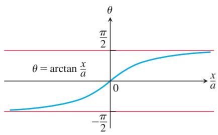
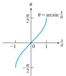
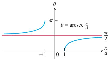
FIGURE 8.3 The arctangent, arcsine, and arcsecant of x/a, graphed as functions of x/a.

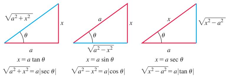
Trigonometric substitutions occur when we replace the variable of integration by a trigonometric function. The most common substitutions are $𝑥 = 𝑎 t a n 𝜃$ , $𝑥 = 𝑎 s i n 𝜃$ , and $𝑥 = 𝑎 s e c 𝜃$ . These substitutions are effective in transforming integrals involving $\sqrt 𝑎 2 + 𝑥 2$ , $\sqrt 𝑎 2 - 𝑥 2$ , and $\sqrt 𝑥 2 - 𝑎 2$ into integrals with respect to $𝜃$ , since they come from the reference right triangles in Figure 8.2.

教材插图

FIGURE 8.2 Reference triangles for the three basic substitutions, identifying the sides labeled x and a for each substitution.

With $𝑥 = 𝑎 t a n 𝜃$ ,

𝑎 2 + 𝑥 2 = 𝑎 2 + 𝑎 2 t a n 2 𝜃 = 𝑎 2 (1 + t a n 2 𝜃) = 𝑎 2 s e c 2 𝜃 .

With $𝑥 = 𝑎 s i n 𝜃$

𝑎 2 - 𝑥 2 = 𝑎 2 - 𝑎 2 s i n 2 𝜃 = 𝑎 2 (1 - s i n 2 𝜃) = 𝑎 2 c o s 2 𝜃 .

With $𝑥 = 𝑎 s e c 𝜃$

𝑥 2 - 𝑎 2 = 𝑎 2 s e c 2 𝜃 - 𝑎 2 = 𝑎 2 (s e c 2 𝜃 - 1) = 𝑎 2 t a n 2 𝜃 .

We want any substitution we use in an integration to be reversible so that we can change back to the original variable afterward. For example, if $𝑥 = 𝑎 t a n 𝜃$ , we want to be able to set $𝜃 = a r c t a n (𝑥 / 𝑎)$ after the integration takes place. If $𝑥 = 𝑎 s i n 𝜃$ , we want to be able to set $𝜃 = a r c s i n (𝑥 / 𝑎)$ when we’re done, and similarly for $𝑥 = 𝑎 s e c 𝜃$ .

As we know from Section 1.5, the functions in these substitutions have inverses only for selected values of $𝜃$ (Figure 8.3). For reversibility,

𝑥 = 𝑎 t a n 𝜃 r e q u i r e s 𝜃 = a r c t a n (𝑥 𝑎) w i t h - 𝜋 2 < 𝜃 < 𝜋 2,

𝑥 = 𝑎 s i n 𝜃 r e q u i r e s 𝜃 = a r c s i n (𝑥 𝑎) w i t h - 𝜋 2 \leq 𝜃 \leq 𝜋 2,

with

{0 \leq 𝜃 < 𝜋 2 i f 𝑥 𝑎 \geq 1, 𝜋 2 < 𝜃 \leq 𝜋 i f 𝑥 𝑎 \leq - 1 .

To simplify calculations with the substitution $𝑥 = 𝑎 s e c 𝜃$ , we will restrict its use to integrals in which $𝑥 / 𝑎 \geq 1$ . This will place $𝜃$ in $[0, 𝜋 / 2)$ and make $t a n 𝜃 \geq 0$ . We will then have $\sqrt 𝑥 2 - 𝑎 2 = \sqrt 𝑎 2 t a n 2 𝜃 = | 𝑎 t a n 𝜃 | = 𝑎 t a n 𝜃$ , free of absolute values, provided $𝑎 > 0$ .

Procedure for a Trigonometric Substitution

Write down the substitution for x, calculate the differential dx, and specify the selected values of $𝜃$ for the substitution.
Substitute the trigonometric expression and the calculated differential into the integrand, and then simplify the results algebraically.
Evaluate the trigonometric integral, keeping in mind the restrictions on the angle $𝜃$ for reversibility.
Draw an appropriate reference triangle to reverse the substitution in the integration result and convert it back to the original variable x.

EXAMPLE 1 Evaluate

\int 𝑑 𝑥 \sqrt 4 + 𝑥 2 .

教材插图

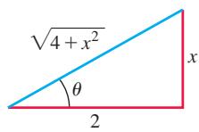
FIGURE 8.4 Reference triangle for $𝑥 = 2 t a n 𝜃$ (Example 1):

t a n 𝜃 = 𝑥 2

Solution We set

and

s e c 𝜃 = \sqrt 4 + 𝑥 2 2 .

Then

𝑥 = 2 t a n 𝜃, 𝑑 𝑥 = 2 s e c 2 𝜃 𝑑 𝜃, - 𝜋 2 < 𝜃 < 𝜋 2, 4 + 𝑥 2 = 4 + 4 t a n 2 𝜃 = 4 (1 + t a n 2 𝜃) = 4 s e c 2 𝜃 .

\int 𝑑 𝑥 \sqrt 4 + 𝑥 2 = \int 2 s e c 2 𝜃 𝑑 𝜃 \sqrt 4 s e c 2 𝜃 = \int s e c 2 𝜃 𝑑 𝜃 | s e c 𝜃 | \sqrt s e c 2 𝜃 = | s e c 𝜃 | = \int s e c 𝜃 𝑑 𝜃 s e c 𝜃 > 0 f o r - 𝜋 2 < 𝜃 < 𝜋 2 = l n | s e c 𝜃 + t a n 𝜃 | + 𝐶 = l n ∣ \sqrt 4 + 𝑥 2 2 + 𝑥 2 ∣ + 𝐶 . F r o m F i g . 8.4

Notice how we expressed $l n | s e c 𝜃 + t a n 𝜃 |$ in terms of x: We drew a reference triangle for the original substitution $𝑥 = 2 t a n 𝜃$ (Figure 8.4) and read the ratios from the triangle.

EXAMPLE 2 Here we find an expression for the inverse hyperbolic sine function in terms of the natural logarithm. Following the same procedure as in Example 1, we find that

\int 𝑑 𝑥 \sqrt 𝑎 2 + 𝑥 2 = \int s e c 𝜃 𝑑 𝜃 = l n | s e c 𝜃 + t a n 𝜃 | + 𝐶 = l n ∣ \sqrt 𝑎 2 + 𝑥 2 𝑎 + 𝑥 𝑎 ∣ + 𝐶 𝑥 = 𝑎 t a n 𝜃, 𝑑 𝑥 = 𝑎 s e c 2 𝜃 𝑑 𝜃 (F i g . 8.2)

From Table 7.9, $s i n h - 1 (𝑥 / 𝑎)$ is also an antiderivative of $1 / \sqrt 𝑎 2 + 𝑥 2$ , so the two anti-derivatives differ by a constant, giving

s i n h - 1 𝑥 𝑎 = l n ∣ \sqrt 𝑎 2 + 𝑥 2 𝑎 + 𝑥 𝑎 ∣ + 𝐶 .

Setting $𝑥 = 0$ in this last equation, we find that $0 = l n | 1 | + 𝐶$ , so $𝐶 = 0$ . Since $\sqrt 𝑎 2 + 𝑥 2 > | 𝑥 |$ , we conclude that $\sqrt 𝑎 2 + 𝑥 2 𝑎 + 𝑥 𝑎 > 0$ , and therefore

s i n h - 1 𝑥 𝑎 = l n (\sqrt 𝑎 2 + 𝑥 2 𝑎 + 𝑥 𝑎)

(See also Exercise 76 in Section 7.3.)

EXAMPLE 3 Evaluate

FIGURE 8.5 Reference triangle for $𝑥 = 3 s i n 𝜃$ (Example 3):

教材插图

s i n 𝜃 = 𝑥 3

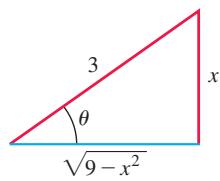
and

\int 𝑥 2 𝑑 𝑥 \sqrt 9 - 𝑥 2 .

Solution We set

c o s 𝜃 = \sqrt 9 - 𝑥 2 3 .

𝑥 = 3 s i n 𝜃, 𝑑 𝑥 = 3 c o s 𝜃 𝑑 𝜃, - 𝜋 2 < 𝜃 < 𝜋 2

Then

9 - 𝑥 2 = 9 - 9 s i n 2 𝜃 = 9 (1 - s i n 2 𝜃) = 9 c o s 2 𝜃 .

\int 𝑥 2 𝑑 𝑥 \sqrt 9 - 𝑥 2 = \int 9 s i n 2 𝜃 \cdot 3 c o s 𝜃 𝑑 𝜃 | 3 c o s 𝜃 | = 9 \int s i n 2 𝜃 𝑑 𝜃 c o s 𝜃 > 0 f o r - 𝜋 2 < 𝜃 < 𝜋 2 = 9 \int 1 - c o s 2 𝜃 2 𝑑 𝜃 s i n 2 𝜃 = 1 - c o s 2 𝜃 2 = 92 (𝜃 - s i n 2 𝜃 2) + 𝐶 = 92 (𝜃 - s i n 𝜃 c o s 𝜃) + 𝐶 s i n 2 𝜃 = 2 s i n 𝜃 c o s 𝜃 = 92 (a r c s i n 𝑥 3 - 𝑥 3 \cdot \sqrt 9 - 𝑥 2 3) + 𝐶 F r o m F i g . 8.5 = 92 a r c s i n 𝑥 3 - 𝑥 2 \sqrt 9 - 𝑥 2 + 𝐶 .

EXAMPLE 4 Evaluate

\int 𝑑 𝑥 \sqrt 25 𝑥 2 - 4, 𝑥 > 25 .

Solution We first rewrite the radical as

\sqrt 25 𝑥 2 - 4 = \sqrt 25 (𝑥 2 - 425) = 5 \sqrt 𝑥 2 - (25) 2 \sqrt 𝑥 2 - 𝑎 2 w i t h 𝑎 = 25

to put the radicand in the form $𝑥 2 - 𝑎 2$ . We then substitute

𝑥 = 25 s e c 𝜃, 𝑑 𝑥 = 25 s e c 𝜃 t a n 𝜃 𝑑 𝜃, 0 < 𝜃 < 𝜋 2 .

We then get

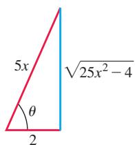
𝑥 2 - (25) 2 = 425 s e c 2 𝜃 - 425 = 425 (s e c 2 𝜃 - 1) = 425 t a n 2 𝜃

教材插图

and

\sqrt 𝑥 2 - (25) 2 = 25 | t a n 𝜃 | = 25 t a n 𝜃 . t a n 𝜃 > 0 f o r 0 < 𝜃 < 𝜋 / 2

With these substitutions, we have

FIGURE 8.6 If $𝑥 = (2 / 5) s e c 𝜃$ ,

$0 < 𝜃 < 𝜋 / 2$ , then $𝜃 = a r c s e c (5 𝑥 / 2)$ ,

and we can read the values of the other trigonometric functions of $𝜃$ from this right triangle (Example 4).

$\int 𝑑 𝑥 \sqrt 25 𝑥 2 - 4 = \int 𝑑 𝑥 5 \sqrt 𝑥 2 - (4 / 25) = \int (2 / 5) s e c 𝜃 t a n 𝜃 𝑑 𝜃 5 \cdot (2 / 5) t a n 𝜃$ $= 15 \int s e c 𝜃 𝑑 𝜃 = 15 l n | s e c 𝜃 + t a n 𝜃 | + 𝐶$ $= 15 l n ∣ 5 𝑥 2 + \sqrt 25 𝑥 2 - 4 2 ∣ + 𝐶 .$ From Fig.8.6

EXERCISES 8.4

Using Trigonometric Substitutions

Evaluate the integrals in Exercises 1–14.

$\int 𝑑 𝑥 \sqrt 9 + 𝑥 2$
$\int 3 𝑑 𝑥 \sqrt 1 + 9 𝑥 2$
$\int 2 - 2 𝑑 𝑥 4 + 𝑥 2$
$\int 20 𝑑 𝑥 8 + 2 𝑥 2$
$\int 3 / 2 0 𝑑 𝑥 \sqrt 9 - 𝑥 2$
$\int 1 / 2 \sqrt 2 0 2 𝑑 𝑥 \sqrt 1 - 4 𝑥 2$
$\int \sqrt 25 - 𝑡 2 𝑑 𝑡$
$\int \sqrt 1 - 9 𝑡 2 𝑑 𝑡$
$\int 𝑑 𝑥 \sqrt 4 𝑥 2 - 49, 𝑥 > 72$
$\int 5 𝑑 𝑥 \sqrt 25 𝑥 2 - 9, 𝑥 > 35$
$\int \sqrt 𝑦 2 - 49 𝑦 𝑑 𝑦, 𝑦 > 7$
$\int \sqrt 𝑦 2 - 25 𝑦 3 𝑑 𝑦, 𝑦 > 5$
$\int 𝑑 𝑥 𝑥 2 \sqrt 𝑥 2 - 1, 𝑥 > 1$
$\int 2 𝑑 𝑥 𝑥 3 \sqrt 𝑥 2 - 1, 𝑥 > 1$

Assorted Integrations

Use any method to evaluate the integrals in Exercises 15–38. Most will require trigonometric substitutions, but some can be evaluated by other methods.

$\int 𝑑 𝑥 𝑥 \sqrt 𝑥 2 - 1$
$\int 𝑑 𝑥 1 + 𝑥 2$
$\int 𝑥 𝑑 𝑥 \sqrt 𝑥 2 - 1$
$\int 𝑑 𝑥 \sqrt 1 - 𝑥 2$
$\int 𝑥 \sqrt 9 - 𝑥 2 𝑑 𝑥$
$\int 𝑥 2 4 + 𝑥 2 𝑑 𝑥$
$\int 𝑥 3 𝑑 𝑥 \sqrt 𝑥 2 + 4$
$\int 𝑑 𝑥 𝑥 2 \sqrt 𝑥 2 + 1$
$\int 8 𝑑 𝑤 𝑤 2 \sqrt 4 - 𝑤 2$
$\int \sqrt 9 - 𝑤 2 𝑤 2 𝑑 𝑤$
$\int \sqrt 𝑥 + 1 1 - 𝑥 𝑑 𝑥$
$\int 𝑥 \sqrt 𝑥 2 - 4 𝑑 𝑥$
$\int \sqrt 3 / 2 0 4 𝑥 2 𝑑 𝑥 (1 - 𝑥 2) 3 / 2$
$\int 10 𝑑 𝑥 (4 - 𝑥 2) 3 / 2$
$\int 𝑑 𝑥 (𝑥 2 - 1) 3 / 2, 𝑥 > 1$
$\int 𝑥 2 𝑑 𝑥 (𝑥 2 - 1) 5 / 2, 𝑥 > 1$
$\int (1 - 𝑥 2) 3 / 2 𝑥 6 𝑑 𝑥$
$\int (1 - 𝑥 2) 1 / 2 𝑥 4 𝑑 𝑥$
$\int 8 𝑑 𝑥 (4 𝑥 2 + 1) 2$
$\int 6 𝑑 𝑡 (9 𝑡 2 + 1) 2$
$\int 𝑥 3 𝑑 𝑥 𝑥 2 - 1$
$\int 𝑥 𝑑 𝑥 25 + 4 𝑥 2$
$\int 𝑣 2 𝑑 𝑣 (1 - 𝑣 2) 5 / 2$
$\int (1 - 𝑟 2) 5 / 2 𝑟 8 𝑑 𝑟$

In Exercises 39–48, use an appropriate substitution and then a trigonometric substitution to evaluate the integrals.

$\int l n 4 0 𝑒 𝑡 𝑑 𝑡 \sqrt 𝑒 2 𝑡 + 9$
$\int l n (4 / 3) l n (3 / 4) 𝑒 𝑡 𝑑 𝑡 (1 + 𝑒 2 𝑡) 3 / 2$
$\int 1 / 4 1 / 12 2 𝑑 𝑡 \sqrt 𝑡 + 4 𝑡 \sqrt 𝑡$
$\int 𝑒 1 𝑑 𝑦 𝑦 \sqrt 1 + (l n 𝑦) 2$
$\int 𝑥 𝑑 𝑥 \sqrt 1 + 𝑥 4$
$\int \sqrt 1 - (l n 𝑥) 2 𝑥 l n 𝑥 𝑑 𝑥$
$\int \sqrt 4 - 𝑥 𝑥 𝑑 𝑥$
$\int \sqrt 𝑥 1 - 𝑥 3 𝑑 𝑥$ (Hint: Let $𝑥 = 𝑢 2$ .)

(Hint: Let $𝑢 = 𝑥 3 / 2$ .)

$\int \sqrt 𝑥 \sqrt 1 - 𝑥 𝑑 𝑥$
$\int \sqrt 𝑥 - 2 \sqrt 𝑥 - 1 𝑑 𝑥$

Complete the Square Before Using Trigonometric Substitutions For Exercises 49–52, complete the square before using an appropriate trigonometric substitution. 49. $\int \sqrt 8 - 2 𝑥 - 𝑥 2 𝑑 𝑥$

$\int 1 \sqrt 𝑥 2 - 2 𝑥 + 5 𝑑 𝑥$
$\int \sqrt 𝑥 2 + 4 𝑥 + 3 𝑥 + 2 𝑑 𝑥$
$\int \sqrt 𝑥 2 + 2 𝑥 + 2 𝑥 2 + 2 𝑥 + 1 𝑑 𝑥$

Initial Value Problems

Initial Value Problems Solve the initial value problems in Exercises 53–56 for y as a function of x. 53. $𝑥 𝑑 𝑦 𝑑 𝑥 = \sqrt 𝑥 2 - 4, 𝑥 \geq 2, 𝑦 (2) = 0$

$\sqrt 𝑥 2 - 9 𝑑 𝑦 𝑑 𝑥 = 1, 𝑥 > 3, 𝑦 (5) = l n 3$
$(𝑥 2 + 4) 𝑑 𝑦 𝑑 𝑥 = 3, 𝑦 (2) = 0$
$(𝑥 2 + 1) 2 𝑑 𝑦 𝑑 𝑥 = \sqrt 𝑥 2 + 1, 𝑦 (0) = 1$

Applications and Examples

Area Find the area of the region in the first quadrant that is enclosed by the coordinate axes and the curve $𝑦 = \sqrt 9 - 𝑥 2 / 3$ .
Area Find the area enclosed by the ellipse $𝑥 2 𝑎 2 + 𝑦 2 𝑏 2 = 1 .$
Consider the region bounded by the graphs of $𝑦 = s i n - 1 𝑥$ , $𝑦 = 0$ , and $𝑥 = 1 / 2$ .
a. Find the area of the region.
b. Find the centroid of the region.
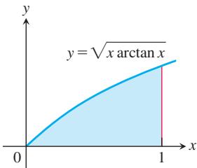
Consider the region bounded by the graphs of $𝑦 = \sqrt 𝑥 a r c t a n 𝑥$ and y = 0 for $0 \leq 𝑥 \leq 1$ . Find the volume of the solid formed by revolving this region about the x-axis (see accompanying figure).

教材插图

Evaluate $\int 𝑥 3 \sqrt 1 - 𝑥 2 𝑑 𝑥$ using a. integration by parts. b. a $𝑢$ -substitution. c. a trigonometric substitution.
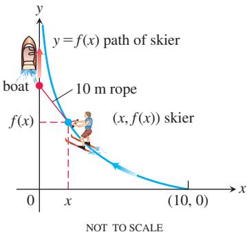
Path of a water skier Suppose that a boat is positioned at the origin with a water skier tethered to the boat at the point (10, 0) on a rope $10 m$ long. As the boat travels along the positive $𝑦$ -axis, the skier is pulled behind the boat along an unknown path $𝑦 = 𝑓 (𝑥)$ , as shown in the accompanying figure.
a. Show that $𝑓' (𝑥) = - \sqrt 100 - 𝑥 2 𝑥$ .
(Hint: Assume that the skier is always pointed directly at the boat and the rope is on a line tangent to the path $𝑦 = 𝑓 (𝑥)$ .)
b. Solve the equation in part (a) for $𝑓 (𝑥)$ , using $𝑓 (10) = 0$ .

教材插图

Find the average value of $𝑓 (𝑥) = \sqrt 𝑥 + 1 \sqrt 𝑥$ on the interval [1, 3].
Find the length of the curve $𝑦 = 1 - 𝑒 - 𝑥$ , $0 \leq 𝑥 \leq 1$ .

8.5 Integration of Rational Functions by Partial Fractions

This section shows how to express a rational function (a quotient of polynomials) as a sum of simpler fractions, called partial fractions, which are more easily integrated. For instance, the rational function $(5 𝑥 - 3) / (𝑥 2 - 2 𝑥 - 3)$ can be rewritten as

5 𝑥 - 3 𝑥 2 - 2 𝑥 - 3 = 2 𝑥 + 1 + 3 𝑥 - 3 .

You can verify this equation algebraically by placing the fractions on the right side over a common denominator $(𝑥 + 1) (𝑥 - 3)$ . The skill acquired in writing rational functions as such a sum is useful in other settings as well (for instance, when using certain transform methods to solve differential equations). To integrate the rational function $(5 𝑥 - 3) / (𝑥 2 - 2 𝑥 - 3)$ on the left side of the expression we are considering, we simply sum the integrals of the fractions on the right side:

\int 5 𝑥 - 3 (𝑥 + 1) (𝑥 - 3) 𝑑 𝑥 = \int 2 𝑥 + 1 𝑑 𝑥 + \int 3 𝑥 - 3 𝑑 𝑥 = 2 l n | 𝑥 + 1 | + 3 l n | 𝑥 - 3 | + 𝐶 .

The method for rewriting rational functions as a sum of simpler fractions is called the method of partial fractions. In the case of our example, it consists of finding constants A and B such that

5 𝑥 - 3 𝑥 2 - 2 𝑥 - 3 = 𝐴 𝑥 + 1 + 𝐵 𝑥 - 3 . (1)

(Pretend for a moment that we do not know that A = 2 and B = 3 will work.) We call the fractions $𝐴 / (𝑥 + 1)$ and $𝐵 / (𝑥 - 3)$ partial fractions because their denominators are only part of the original denominator $𝑥 2 - 2 𝑥 - 3$ . We call A and B undetermined coefficients until suitable values for them have been found.

To find $𝐴$ and $𝐵$ , we first clear Equation (1) of fractions and regroup in powers of $𝑥$ , obtaining

5 𝑥 - 3 = 𝐴 (𝑥 - 3) + 𝐵 (𝑥 + 1) = (𝐴 + 𝐵) 𝑥 - 3 𝐴 + 𝐵 .

This will be an identity in $𝑥$ if and only if the coefficients of like powers of $𝑥$ on the two sides are equal:

𝐴 + 𝐵 = 5, - 3 𝐴 + 𝐵 = - 3 .

Solving these equations simultaneously gives A = 2 and B = 3.

General Description of the Method

Success in writing a rational function $𝑓 (𝑥) / 𝑔 (𝑥)$ as a sum of partial fractions depends on three things:

The degree of $𝑓 (𝑥)$ must be less than the degree of $𝑔 (𝑥)$ . That is, the fraction must be proper. If it isn’t, divide $𝑓 (𝑥)$ by $𝑔 (𝑥)$ and work with the remainder term. Example 3 of this section illustrates such a case.
We must know the factors of $𝑔 (𝑥)$ . In theory, any polynomial with real coefficients can be written as a product of real linear factors and real quadratic factors. In practice, the factors may be hard to find.
The values of the undetermined coefficients form a system of $𝑛$ linear equations in $𝑛$ unknowns. For large $𝑛$ , solving such systems may require linear algebra methods (such as Gaussian Elimination).

Here is how we find the partial fractions of a proper fraction $𝑓 (𝑥) / 𝑔 (𝑥)$ when the factors of g are known. A quadratic polynomial (or factor) is irreducible if it cannot be written as the product of two linear factors with real coefficients. That is, the polynomial has no real roots.

Method of Partial Fractions When $𝑓 (𝑥) / 𝑔 (𝑥)$ Is Proper

Let $𝑥 - 𝑟$ be a linear factor of $𝑔 (𝑥)$ . Suppose that $(𝑥 - 𝑟) 𝑚$ is the highest power of $𝑥 - 𝑟$ that divides $𝑔 (𝑥)$ . Then, to this factor, assign the sum of the $𝑚$ partial fractions:

𝐴 1 (𝑥 - 𝑟) + 𝐴 2 (𝑥 - 𝑟) 2 + \dots + 𝐴 𝑚 (𝑥 - 𝑟) 𝑚 .

Do this for each distinct linear factor of $𝑔 (𝑥)$ .

Let $𝑥 2 + 𝑝 𝑥 + 𝑞$ be an irreducible quadratic factor of $𝑔 (𝑥)$ . In this case, $𝑥 2 + 𝑝 𝑥 + 𝑞$ has no real roots. Suppose that $(𝑥 2 + 𝑝 𝑥 + 𝑞) 𝑛$ is the highest power of this factor that divides $𝑔 (𝑥)$ . Then, to this factor, assign the sum of the n partial fractions:

𝐵 1 𝑥 + 𝐶 1 (𝑥 2 + 𝑝 𝑥 + 𝑞) + 𝐵 2 𝑥 + 𝐶 2 (𝑥 2 + 𝑝 𝑥 + 𝑞) 2 + \dots + 𝐵 𝑛 𝑥 + 𝐶 𝑛 (𝑥 2 + 𝑝 𝑥 + 𝑞) 𝑛 .

Do this for each distinct quadratic factor of $𝑔 (𝑥)$ .

Set the original fraction $𝑓 (𝑥) / 𝑔 (𝑥)$ equal to the sum of all these partial fractions. Clear the resulting equation of fractions.
Find the values of the undetermined coefficients.

There are often multiple ways to find the values of the undetermined coefficients in Step 4. To find the values of the coefficients that satisfy Equation (1), we equated coefficients of like powers of x. In the next example, we instead will assign convenient values of x, leading to simple equations that we can solve for the undetermined coefficients.

EXAMPLE 1 Use partial fractions to evaluate

\int 𝑥 2 + 4 𝑥 + 1 (𝑥 - 1) (𝑥 + 1) (𝑥 + 3) 𝑑 𝑥 .

Solution Note that each of the factors $(𝑥 - 1)$ , $(𝑥 + 1)$ , and $(𝑥 + 3)$ is raised only to the first power. Therefore, the partial fraction decomposition has the form

𝑥 2 + 4 𝑥 + 1 (𝑥 - 1) (𝑥 + 1) (𝑥 + 3) = 𝐴 𝑥 - 1 + 𝐵 𝑥 + 1 + 𝐶 𝑥 + 3 .

To find the values of the undetermined coefficients A, B, and C, we clear fractions and get

𝑥 2 + 4 𝑥 + 1 = 𝐴 (𝑥 + 1) (𝑥 + 3) + 𝐵 (𝑥 - 1) (𝑥 + 3) + 𝐶 (𝑥 - 1) (𝑥 + 1) .

On the right side, we notice that a factor $(𝑥 - 1)$ is present in all terms except for the one containing A. Therefore, letting x = 1 allows us to solve for A.

𝑥 = 1 : 12 + 4 (1) + 1 = 𝐴 (2) (4) + 𝐵 (0) + 𝐶 (0)

6 = 8 𝐴

𝐴 = 34

In a similar manner, we can let x equal -1 to find B or -3 to find C.

𝑥 = - 1 : (- 1) 2 + 4 (- 1) + 1 = 𝐴 (0) + 𝐵 (- 2) (2) + 𝐶 (0) - 2 = - 4 𝐵

𝐵 = 12

𝑥 = - 3 : (- 3) 2 + 4 (- 3) + 1 = 𝐴 (0) + 𝐵 (0) + 𝐶 (- 4) (- 2) - 2 = 8 𝐶

𝐶 = - 14

Hence we have

\int 𝑥 2 + 4 𝑥 + 1 (𝑥 - 1) (𝑥 + 1) (𝑥 + 3) 𝑑 𝑥 = \int [34 1 𝑥 - 1 + 12 1 𝑥 + 1 - 14 1 𝑥 + 3] 𝑑 𝑥 = 34 l n | 𝑥 - 1 | + 12 l n | 𝑥 + 1 | - 14 l n | 𝑥 + 3 | + 𝐾,

where K is the arbitrary constant of integration (we call it K here to avoid confusion with the undetermined coefficient we labeled as C).

You can solve for the undetermined coefficients $(𝐴, 𝐵, e t c .)$ by equating coefficients of like powers of x or by assigning convenient values to x. You should choose the method that is most convenient for the problem at hand.

EXAMPLE 2 Use partial fractions to evaluate

\int 6 𝑥 + 7 (𝑥 + 2) 2 𝑑 𝑥 .

Solution First we express the integrand as a sum of partial fractions with undetermined coefficients.

6 𝑥 + 7 (𝑥 + 2) 2 = 𝐴 𝑥 + 2 + 𝐵 (𝑥 + 2) 2 T w o t e r m s b e c a u s e (𝑥 + 2) i s s q u a r e d 6 𝑥 + 7 = 𝐴 (𝑥 + 2) + 𝐵 M u l t i p l y b o t h s i d e s b y (𝑥 + 2) 2 . = 𝐴 𝑥 + (2 𝐴 + 𝐵)

Equating coefficients of corresponding powers of x gives

𝐴 = 6 a n d 2 𝐴 + 𝐵 = 12 + 𝐵 = 7, o r 𝐴 = 6 a n d 𝐵 = - 5 .

Therefore,

\int 6 𝑥 + 7 (𝑥 + 2) 2 𝑑 𝑥 = \int (6 𝑥 + 2 - 5 (𝑥 + 2) 2) 𝑑 𝑥 = 6 \int 𝑑 𝑥 𝑥 + 2 - 5 \int (𝑥 + 2) - 2 𝑑 𝑥 = 6 l n | 𝑥 + 2 | + 5 (𝑥 + 2) - 1 + 𝐶 .

The next example shows how to handle the case when $𝑓 (𝑥) / 𝑔 (𝑥)$ is an improper fraction. It is a case where the degree of f is larger than the degree of g.

EXAMPLE 3 Use partial fractions to evaluate

\int 2 𝑥 3 - 4 𝑥 2 - 𝑥 - 3 𝑥 2 - 2 𝑥 - 3 𝑑 𝑥 .

Solution First we divide the denominator into the numerator to get a polynomial plus a proper fraction.

𝑥 2 - 2 𝑥 - 3 ――――――――――) 2 𝑥 3 - 4 𝑥 2 - 𝑥 - 3 2 𝑥 3 - 4 𝑥 2 - 6 𝑥 ―――――――― 5 𝑥 - 3

Then we write the improper fraction as a polynomial plus a proper fraction.

2 𝑥 3 - 4 𝑥 2 - 𝑥 - 3 𝑥 2 - 2 𝑥 - 3 = 2 𝑥 + 5 𝑥 - 3 𝑥 2 - 2 𝑥 - 3

We found the partial fraction decomposition of the fraction on the right in the opening example, so

\int 2 𝑥 3 - 4 𝑥 2 - 𝑥 - 3 𝑥 2 - 2 𝑥 - 3 𝑑 𝑥 = \int 2 𝑥 𝑑 𝑥 + \int 5 𝑥 - 3 𝑥 2 - 2 𝑥 - 3 𝑑 𝑥 = \int 2 𝑥 𝑑 𝑥 + \int 2 𝑥 + 1 𝑑 𝑥 + \int 3 𝑥 - 3 𝑑 𝑥 = 𝑥 2 + 2 l n | 𝑥 + 1 | + 3 l n | 𝑥 - 3 | + 𝐶 .

EXAMPLE 4 Use partial fractions to evaluate

\int - 2 𝑥 + 4 (𝑥 2 + 1) (𝑥 - 1) 2 𝑑 𝑥 .

Solution The denominator has an irreducible quadratic factor $𝑥 2 + 1$ as well as a repeated linear factor $(𝑥 - 1) 2$ , so we write

- 2 𝑥 + 4 (𝑥 2 + 1) (𝑥 - 1) 2 = 𝐴 𝑥 + 𝐵 𝑥 2 + 1 + 𝐶 𝑥 - 1 + 𝐷 (𝑥 - 1) 2 . (2)

Clearing the equation of fractions gives

- 2 𝑥 + 4 = (𝐴 𝑥 + 𝐵) (𝑥 - 1) 2 + 𝐶 (𝑥 - 1) (𝑥 2 + 1) + 𝐷 (𝑥 2 + 1) = (𝐴 + 𝐶) 𝑥 3 + (- 2 𝐴 + 𝐵 - 𝐶 + 𝐷) 𝑥 2 + (𝐴 - 2 𝐵 + 𝐶) 𝑥 + (𝐵 - 𝐶 + 𝐷) .

Equating coefficients of like terms gives

C o e f f i c i e n t s o f 𝑥 3 : 0 = 𝐴 + 𝐶

C o e f f i c i e n t s o f 𝑥 2 : 0 = - 2 𝐴 + 𝐵 - 𝐶 + 𝐷

C o e f f i c i e n t s o f 𝑥 1 : - 2 = 𝐴 - 2 𝐵 + 𝐶

C o e f f i c i e n t s o f 𝑥 0 : 4 = 𝐵 - 𝐶 + 𝐷

We solve these equations simultaneously to find the values of A, B, C, and D.

- 4 = - 2 𝐴, 𝐴 = 2 S u b t r a c t f o u r t h e q u a t i o n f r o m s e c o n d .

𝐶 = - 𝐴 = - 2 F r o m t h e f i r s t e q u a t i o n

𝐵 = (𝐴 + 𝐶 + 2) / 2 = 1 F r o m t h e t h i r d e q u a t i o n a n d 𝐶 = - 𝐴

𝐷 = 4 - 𝐵 + 𝐶 = 1 . F r o m t h e f o u r t h e q u a t i o n

We substitute these values into Equation (2), obtaining

- 2 𝑥 + 4 (𝑥 2 + 1) (𝑥 - 1) 2 = 2 𝑥 + 1 𝑥 2 + 1 - 2 𝑥 - 1 + 1 (𝑥 - 1) 2 .

Finally, using the expansion above, we can integrate:

\int - 2 𝑥 + 4 (𝑥 2 + 1) (𝑥 - 1) 2 𝑑 𝑥 = \int (2 𝑥 + 1 𝑥 2 + 1 - 2 𝑥 - 1 + 1 (𝑥 - 1) 2) 𝑑 𝑥 = \int (2 𝑥 𝑥 2 + 1 + 1 𝑥 2 + 1 - 2 𝑥 - 1 + 1 (𝑥 - 1) 2) 𝑑 𝑥 = l n (𝑥 2 + 1) + t a n - 1 𝑥 - 2 l n | 𝑥 - 1 | - 1 𝑥 - 1 + 𝐾 .

We use the letter K instead of C to represent an arbitrary constant here because we have already used C to represent a variable in the partial fraction representation.

EXAMPLE 5 Use partial fractions to evaluate

\int 𝑑 𝑥 𝑥 (𝑥 2 + 1) 2 .

Solution The form of the partial fraction decomposition is

1 𝑥 (𝑥 2 + 1) 2 = 𝐴 𝑥 + 𝐵 𝑥 + 𝐶 𝑥 2 + 1 + 𝐷 𝑥 + 𝐸 (𝑥 2 + 1) 2 .

Multiplying by $𝑥 (𝑥 2 + 1) 2$ , we have

1 = 𝐴 (𝑥 2 + 1) 2 + (𝐵 𝑥 + 𝐶) 𝑥 (𝑥 2 + 1) + (𝐷 𝑥 + 𝐸) 𝑥 = 𝐴 (𝑥 4 + 2 𝑥 2 + 1) + 𝐵 (𝑥 4 + 𝑥 2) + 𝐶 (𝑥 3 + 𝑥) + 𝐷 𝑥 2 + 𝐸 𝑥 = (𝐴 + 𝐵) 𝑥 4 + 𝐶 𝑥 3 + (2 𝐴 + 𝐵 + 𝐷) 𝑥 2 + (𝐶 + 𝐸) 𝑥 + 𝐴 .

If we equate coefficients, we get the system

𝐴 + 𝐵 = 0, 𝐶 = 0, 2 𝐴 + 𝐵 + 𝐷 = 0, 𝐶 + 𝐸 = 0, 𝐴 = 1 .

Solving this system gives A = 1, B = -1, C = 0, D = -1, and E = 0. Thus,

HISTORICAL BIOGRAPHY Oliver Heaviside (1850–1925)

Heaviside studied electricity and languages on his own. He was able to simplify Maxwell’s 20 equations into the two we now call Maxwell’s equations. Heaviside’s contributions in mathematics are in the areas of vector algebra and vector calculus.

To know more, visit the companion Website.

\int 𝑑 𝑥 𝑥 (𝑥 2 + 1) 2 = \int [1 𝑥 + - 𝑥 𝑥 2 + 1 + - 𝑥 (𝑥 2 + 1) 2] 𝑑 𝑥 = \int 𝑑 𝑥 𝑥 - \int 𝑥 𝑑 𝑥 𝑥 2 + 1 - \int 𝑥 𝑑 𝑥 (𝑥 2 + 1) 2 = \int 𝑑 𝑥 𝑥 - 12 \int 𝑑 𝑢 𝑢 - 12 \int 𝑑 𝑢 𝑢 2 𝑢 = 𝑥 2 + 1, = l n | 𝑥 | - 12 l n | 𝑢 | + 1 2 𝑢 + 𝐾 = l n | 𝑥 | - 12 l n (𝑥 2 + 1) + 1 2 (𝑥 2 + 1) + 𝐾 = l n | 𝑥 | \sqrt 𝑥 2 + 1 + 1 2 (𝑥 2 + 1) + 𝐾 .

Determining Coefficients by Differentiating

Another way to determine the constants that appear in partial fractions is to differentiate, as in the next example.

EXAMPLE 6 Find $𝐴, 𝐵$ , and $𝐶$ in the equation

𝑥 - 1 (𝑥 + 1) 3 = 𝐴 𝑥 + 1 + 𝐵 (𝑥 + 1) 2 + 𝐶 (𝑥 + 1) 3 .

Solution We first clear fractions:

𝑥 - 1 = 𝐴 (𝑥 + 1) 2 + 𝐵 (𝑥 + 1) + 𝐶 .

Substituting $𝑥 = - 1$ shows $𝐶 = - 2$ . We then differentiate both sides with respect to $𝑥$ , obtaining

1 = 2 𝐴 (𝑥 + 1) + 𝐵 .

Substituting $𝑥 = - 1$ shows $𝐵 = 1$ . We differentiate again to get $0 = 2 𝐴$ , which shows $𝐴 = 0$ . Hence,

𝑥 - 1 (𝑥 + 1) 3 = 1 (𝑥 + 1) 2 - 2 (𝑥 + 1) 3 .

EXERCISES 8.5

Expanding Quotients into Partial Fractions

Expand the quotients in Exercises 1–8 by partial fractions.

$5 𝑥 - 13 (𝑥 - 3) (𝑥 - 2)$
$5 𝑥 - 7 𝑥 2 - 3 𝑥 + 2$
$𝑥 + 4 (𝑥 + 1) 2$
$2 𝑥 + 2 𝑥 2 - 2 𝑥 + 1$
$𝑧 + 1 𝑧 2 (𝑧 - 1)$
$𝑧 𝑧 3 - 𝑧 2 - 6 𝑧$
$𝑡 2 + 8 𝑡 2 - 5 𝑡 + 6$
$𝑡 4 + 9 𝑡 4 + 9 𝑡 2$

Nonrepeated Linear Factors In Exercises 9–16, express the integrand as a sum of partial fractions and evaluate the integrals. 9. $\int 𝑑 𝑥 1 - 𝑥 2$

$\int 𝑑 𝑥 𝑥 2 + 2 𝑥$
$\int 𝑥 + 4 𝑥 2 + 5 𝑥 - 6 𝑑 𝑥$
$\int 2 𝑥 + 1 𝑥 2 - 7 𝑥 + 12 𝑑 𝑥$
$\int 84 𝑦 𝑑 𝑦 𝑦 2 - 2 𝑦 - 3$
$\int 1 1 / 2 𝑦 + 4 𝑦 2 + 𝑦 𝑑 𝑦$
$\int 𝑑 𝑡 𝑡 3 + 𝑡 2 - 2 𝑡$
$\int 𝑥 + 3 2 𝑥 3 - 8 𝑥 𝑑 𝑥$

Repeated Linear Factors

In Exercises 17–20, express the integrand as a sum of partial fractions and evaluate the integrals.

\int 10 𝑥 3 𝑑 𝑥 𝑥 2 + 2 𝑥 + 1

$\int 0 - 1 𝑥 3 𝑑 𝑥 𝑥 2 - 2 𝑥 + 1$
$\int 𝑑 𝑥 (𝑥 2 - 1) 2$
$\int 𝑥 2 𝑑 𝑥 (𝑥 - 1) (𝑥 2 + 2 𝑥 + 1)$

In Exercises 21–32, express the integrand as a sum of partial fractions and evaluate the integrals.

$\int 10 𝑑 𝑥 (𝑥 + 1) (𝑥 2 + 1)$
$\int \sqrt 3 1 3 𝑡 2 + 𝑡 + 4 𝑡 3 + 𝑡 𝑑 𝑡$
$\int 𝑦 2 + 2 𝑦 + 1 (𝑦 2 + 1) 2 𝑑 𝑦$
$\int 8 𝑥 2 + 8 𝑥 + 2 (4 𝑥 2 + 1) 2 𝑑 𝑥$
$\int 2 𝑠 + 2 (𝑠 2 + 1) (𝑠 - 1) 3 𝑑 𝑠$
$\int 𝑠 4 + 81 𝑠 (𝑠 2 + 9) 2 𝑑 𝑠$
$\int 𝑥 2 - 𝑥 + 2 𝑥 3 - 1 𝑑 𝑥$
$\int 1 𝑥 4 + 𝑥 𝑑 𝑥$
$\int 𝑥 2 𝑥 4 - 1 𝑑 𝑥$
$\int 𝑥 2 + 𝑥 𝑥 4 - 3 𝑥 2 - 4 𝑑 𝑥$
$\int 2 𝜃 3 + 5 𝜃 2 + 8 𝜃 + 4 (𝜃 2 + 2 𝜃 + 2) 2 𝑑 𝜃$
$\int 𝜃 4 - 4 𝜃 3 + 2 𝜃 2 - 3 𝜃 + 1 (𝜃 2 + 1) 3 𝑑 𝜃$

Improper Fractions

In Exercises 33–38, perform long division on the integrand, write the proper fraction as a sum of partial fractions, and then evaluate the integral.

$\int 2 𝑥 3 - 2 𝑥 2 + 1 𝑥 2 - 𝑥 𝑑 𝑥$
$\int 𝑥 4 𝑥 2 - 1 𝑑 𝑥$
$\int 9 𝑥 3 - 3 𝑥 + 1 𝑥 3 - 𝑥 2 𝑑 𝑥$
$\int 16 𝑥 3 4 𝑥 2 - 4 𝑥 + 1 𝑑 𝑥$
$\int 𝑦 4 + 𝑦 2 - 1 𝑦 3 + 𝑦 𝑑 𝑦$
$\int 2 𝑦 4 𝑦 3 - 𝑦 2 + 𝑦 - 1 𝑑 𝑦$

Evaluating Integrals

Evaluate the integrals in Exercises 39–54.

$\int 𝑒 𝑡 𝑑 𝑡 𝑒 2 𝑡 + 3 𝑒 𝑡 + 2$
$\int 𝑒 4 𝑡 + 2 𝑒 2 𝑡 - 𝑒 𝑡 𝑒 2 𝑡 + 1 𝑑 𝑡$
$\int c o s 𝑦 𝑑 𝑦 s i n 2 𝑦 + s i n 𝑦 - 6$
$\int s i n 𝜃 𝑑 𝜃 c o s 2 𝜃 + c o s 𝜃 - 2$
$\int (𝑥 - 2) 2 t a n - 1 (2 𝑥) - 12 𝑥 3 - 3 𝑥 (4 𝑥 2 + 1) (𝑥 - 2) 2 𝑑 𝑥$
$\int (𝑥 + 1) 2 t a n - 1 (3 𝑥) + 9 𝑥 3 + 𝑥 (9 𝑥 2 + 1) (𝑥 + 1) 2 𝑑 𝑥$
$\int 1 𝑥 3 / 2 - \sqrt 𝑥 𝑑 𝑥$
$\int 1 (𝑥 1 / 3 - 1) \sqrt 𝑥 𝑑 𝑥$ (Hint: Let $𝑥 = 𝑢 6$ .)
$\int \sqrt 𝑥 + 1 𝑥 𝑑 𝑥$
$\int 1 𝑥 \sqrt 𝑥 + 9 𝑑 𝑥$ (Hint: Let $𝑥 + 1 = 𝑢 2$ .)
$\int 1 𝑥 (𝑥 4 + 1) 𝑑 𝑥$ (Hint: Multiply by $𝑥 3 𝑥 3$ .)
$\int 1 𝑥 6 (𝑥 5 + 4) 𝑑 𝑥$
$\int 1 c o s 2 𝜃 s i n 𝜃 𝑑 𝜃$
$\int 1 c o s 𝜃 + s i n 2 𝜃 𝑑 𝜃$
$\int \sqrt 1 + \sqrt 𝑥 𝑥 𝑑 𝑥$
$\int \sqrt 𝑥 \sqrt 2 - \sqrt 𝑥 + \sqrt 𝑥 𝑑 𝑥$

Use any method to evaluate the integrals in Exercises 55–66. 55. $\int 𝑥 3 - 2 𝑥 2 - 3 𝑥 𝑥 + 2 𝑑 𝑥$

$\int 𝑥 + 2 𝑥 3 - 2 𝑥 2 - 3 𝑥 𝑑 𝑥$
$\int 2 𝑥 - 2 - 𝑥 2 𝑥 + 2 - 𝑥 𝑑 𝑥$
$\int 2 𝑥 2 2 𝑥 + 2 𝑥 - 2 𝑑 𝑥$
$\int 1 𝑥 4 - 1 𝑑 𝑥$
$\int 𝑥 4 - 1 𝑥 5 - 5 𝑥 + 1 𝑑 𝑥$
$\int l n 𝑥 + 2 𝑥 (l n 𝑥 + 1) (l n 𝑥 + 3) 𝑑 𝑥$
$\int 2 𝑥 (l n 𝑥 - 2) 3 𝑑 𝑥$
$\int 1 \sqrt 𝑥 2 - 1 𝑑 𝑥$
$\int 𝑥 𝑥 + \sqrt 𝑥 2 + 2 𝑑 𝑥$
$\int 𝑥 5 \sqrt 𝑥 3 + 1 𝑑 𝑥$
$\int 𝑥 2 \sqrt 1 - 𝑥 2 𝑑 𝑥$

Initial Value Problems

Solve the initial value problems in Exercises 67–70 for x as a function of t.

$(𝑡 2 - 3 𝑡 + 2) 𝑑 𝑥 𝑑 𝑡 = 1$ (t>2), $𝑥 (3) = 0$
$(3 𝑡 4 + 4 𝑡 2 + 1) 𝑑 𝑥 𝑑 𝑡 = 2 \sqrt 3$ , $𝑥 (1) = - 𝜋 \sqrt 3 / 4$
$(𝑡 2 + 2 𝑡) 𝑑 𝑥 𝑑 𝑡 = 2 𝑥 + 2$ (t,x>0), $𝑥 (1) = 1$
$(𝑡 + 1) 𝑑 𝑥 𝑑 𝑡 = 𝑥 2 + 1$ (t>-1), $𝑥 (0) = 0$

Applications and Examples

In Exercises 71 and 72, find the volume of the solid generated by revolving the shaded region about the indicated axis.

The $𝑥$ -axis

教材插图

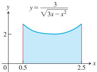
The $𝑦$ -axis

教材插图

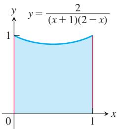
Find the length of the curve $𝑦 = l n (1 - 𝑥 2)$ , $0 \leq 𝑥 \leq 12$ .
Evaluate $\int s e c 𝜃 𝑑 𝜃$ by a. multiplying by $s e c 𝜃 + t a n 𝜃 s e c 𝜃 + t a n 𝜃$ and then using a $𝑢$ -substitution b. writing the integral as $\int 1 c o s 𝜃 𝑑 𝜃$ . Then multiply by $c o s 𝜃 c o s 𝜃$ , use a trigonometric identity and a $𝑢$ -substitution, and finally integrate using partial fractions.

教材插图

T 75. Find, to two decimal places, the $𝑥$ -coordinate of the centroid of the region in the first quadrant bounded by the $𝑥$ -axis, the curve $𝑦 = a r c t a n 𝑥$ , and the line $𝑥 = \sqrt 3$ .

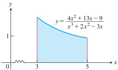
T 76. Find the $𝑥$ -coordinate of the centroid of this region to two decimal places.

教材插图

Social diffusion Sociologists sometimes use the phrase “social diffusion” to describe the way information spreads through a population. The information might be a rumor, a cultural fad, or news about a technical innovation. In a sufficiently large population, the number of people x who have the information is treated as a differentiable function of time t, and the rate of diffusion, dx/dt, is assumed to be proportional to the number of people who have the information times the number of people who do not. This leads to the equation

𝑑 𝑥 𝑑 𝑡 = 𝑘 𝑥 (𝑁 - 𝑥),

where N is the number of people in the population.

Suppose t is in days, k = 1/250, and two people start a rumor at time t = 0 in a population of N = 1000 people.

a. Find x as a function of t.

b. When will half the population have heard the rumor? (This is when the rumor will be spreading the fastest.)

Second-order chemical reactions Many chemical reactions are the result of the interaction of two molecules that undergo a change to produce a new product. The rate of the reaction typically depends on the concentrations of the two kinds of molecules. If $𝑎$ is the amount of substance $𝐴$ and $𝑏$ is the amount of substance $𝐵$ at time $𝑡 = 0$ , and if $𝑥$ is the amount of product at time $𝑡$ , then the rate of formation of $𝑥$ may be given by the differential equation

𝑑 𝑥 𝑑 𝑡 = 𝑘 (𝑎 - 𝑥) (𝑏 - 𝑥),

1 (𝑎 - 𝑥) (𝑏 - 𝑥) 𝑑 𝑥 𝑑 𝑡 = 𝑘,

where k is a constant for the reaction. Integrate both sides of this equation to obtain a relation between x and t (a) if a = b, and (b) if $𝑎 \neq 𝑏$ . Assume in each case that x = 0 when t = 0.

8.6 Integral Tables and Computer Algebra Systems

In this section we discuss how to use tables and computer algebra systems (CAS) to evaluate integrals.

Integral Tables

A Brief Table of Integrals is provided at the back of the text, after the index. (More extensive tables appear in compilations such as CRC Mathematical Tables, which contain thousands of integrals.) The integration formulas are stated in terms of constants a, b, c, m, n, and so on. These constants can usually assume any real value and need not be integers. Occasional limitations on their values are stated with the formulas. Formula 21 requires $𝑛 \neq - 1$ , for example, and Formula 27 requires $𝑛 \neq - 2$ .

The formulas also assume that the constants do not take on values that require dividing by zero or taking even roots of negative numbers. For example, Formula 24 assumes that $𝑎 \neq 0$ , and Formulas 29a and 29b cannot be used unless b is positive.

EXAMPLE 1 Find

\int 𝑥 (2 𝑥 + 5) - 1 𝑑 𝑥 .

Solution We use Formula 24 at the back of the text (not 22, which requires $𝑛 \neq - 1$ ):

\int 𝑥 (𝑎 𝑥 + 𝑏) - 1 𝑑 𝑥 = 𝑥 𝑎 - 𝑏 𝑎 2 l n | 𝑎 𝑥 + 𝑏 | + 𝐶 .

With $𝑎 = 2$ and $𝑏 = 5$ , we have

\int 𝑥 (2 𝑥 + 5) - 1 𝑑 𝑥 = 𝑥 2 - 54 l n | 2 𝑥 + 5 | + 𝐶 .

EXAMPLE 2 Find

\int 𝑑 𝑥 𝑥 \sqrt 2 𝑥 - 4 .

Solution We use Formula 29b:

\int 𝑑 𝑥 𝑥 \sqrt 𝑎 𝑥 - 𝑏 = 2 \sqrt 𝑏 a r c t a n \sqrt 𝑎 𝑥 - 𝑏 𝑏 + 𝐶 .

With $𝑎 = 2$ and $𝑏 = 4$ , we have

\int 𝑑 𝑥 𝑥 \sqrt 2 𝑥 - 4 = 2 \sqrt 4 a r c t a n \sqrt 2 𝑥 - 4 4 + 𝐶 = a r c t a n \sqrt 𝑥 - 2 2 + 𝐶 .

EXAMPLE 3 Find

\int 𝑥 a r c s i n 𝑥 𝑑 𝑥 .

Solution We begin by using Formula 106:

\int 𝑥 𝑛 a r c s i n 𝑎 𝑥 𝑑 𝑥 = 𝑥 𝑛 + 1 𝑛 + 1 a r c s i n 𝑎 𝑥 - 𝑎 𝑛 + 1 \int 𝑥 𝑛 + 1 𝑑 𝑥 \sqrt 1 - 𝑎 2 𝑥 2, 𝑛 \neq - 1 .

With $𝑛 = 1$ and $𝑎 = 1$ , we have

\int 𝑥 a r c s i n 𝑥 𝑑 𝑥 = 𝑥 2 2 a r c s i n 𝑥 - 12 \int 𝑥 2 𝑑 𝑥 \sqrt 1 - 𝑥 2 .

Next we use Formula 49 to find the integral on the right:

\int 𝑥 2 \sqrt 𝑎 2 - 𝑥 2 𝑑 𝑥 = 𝑎 2 2 a r c s i n (𝑥 𝑎) - 12 𝑥 \sqrt 𝑎 2 - 𝑥 2 + 𝐶 .

With a = 1,

\int 𝑥 2 𝑑 𝑥 \sqrt 1 - 𝑥 2 = 12 a r c s i n 𝑥 - 12 𝑥 \sqrt 1 - 𝑥 2 + 𝐶 .

The combined result is

\int 𝑥 a r c s i n 𝑥 𝑑 𝑥 = 𝑥 2 2 a r c s i n 𝑥 - 12 (12 a r c s i n 𝑥 - 12 𝑥 \sqrt 1 - 𝑥 2 + 𝐶) = (𝑥 2 2 - 14) a r c s i n 𝑥 + 14 𝑥 \sqrt 1 - 𝑥 2 + 𝐶' .

Reduction Formulas

The time required for repeated integrations by parts can sometimes be shortened by applying reduction formulas like the following.

\int t a n 𝑛 𝑥 𝑑 𝑥 = 1 𝑛 - 1 t a n 𝑛 - 1 𝑥 - \int t a n 𝑛 - 2 𝑥 𝑑 𝑥 (1)

\int (l n 𝑥) 𝑛 𝑑 𝑥 = 𝑥 (l n 𝑥) 𝑛 - 𝑛 \int (l n 𝑥) 𝑛 - 1 𝑑 𝑥 (2)

\int s i n 𝑛 𝑥 c o s 𝑚 𝑥 𝑑 𝑥 = - s i n 𝑛 - 1 𝑥 c o s 𝑚 + 1 𝑥 𝑚 + 𝑛 + 𝑛 - 1 𝑚 + 𝑛 \int s i n 𝑛 - 2 𝑥 c o s 𝑚 𝑥 𝑑 𝑥 (𝑛 \neq - 𝑚) . (3)

By applying such a formula repeatedly, we can eventually express the original integral in terms of a power low enough to be evaluated directly. The next example illustrates this procedure.

EXAMPLE 4 Find

\int t a n 5 𝑥 𝑑 𝑥 .

Solution We apply Equation (1) with n = 5 to get

\int t a n 5 𝑥 𝑑 𝑥 = 14 t a n 4 𝑥 - \int t a n 3 𝑥 𝑑 𝑥 .

We then apply Equation (1) again, with $𝑛 = 3$ , to evaluate the remaining integral:

\int t a n 3 𝑥 𝑑 𝑥 = 12 t a n 2 𝑥 - \int t a n 𝑥 𝑑 𝑥 = 12 t a n 2 𝑥 + l n | c o s 𝑥 | + 𝐶 1 .

The combined result is

\int t a n 5 𝑥 𝑑 𝑥 = 14 t a n 4 𝑥 - 12 t a n 2 𝑥 - l n | c o s 𝑥 | + 𝐶 .

As their form suggests, reduction formulas are derived using integration by parts. (See Example 5 in Section 8.3.)

Integration with a CAS

A powerful capability of computer algebra systems is their ability to integrate symbolically. This is performed with the integrate command specified by the particular system (for example, int in Maple, Integrate in Mathematica).

EXAMPLE 5 Suppose that you want to evaluate the indefinite integral of the function

𝑓 (𝑥) = 𝑥 2 \sqrt 𝑎 2 + 𝑥 2 .

Using Maple, you first define or name the function:

𝑓 : = 𝑥 \land 2 * s q r t (𝑎 \land 2 + 𝑥 \land 2);

Then you use the integrate command on f, identifying the variable of integration:

i n t (𝑓, 𝑥);

Maple returns the answer

𝑥 (𝑎 2 + 𝑥 2) 3 / 2 4 - 𝑎 2 𝑥 \sqrt 𝑎 2 + 𝑥 2 8 - 𝑎 4 l n (𝑥 + \sqrt 𝑎 2 + 𝑥 2) 8

If you want to see whether the answer can be simplified, enter

s i m p l i f y (%);

Maple returns

- 𝑎 4 l n (𝑥 + \sqrt 𝑎 2 + 𝑥 2) 8 + 𝑥 \sqrt 𝑎 2 + 𝑥 2 (𝑎 2 + 2 𝑥 2) 8

If you want the definite integral for $0 \leq 𝑥 \leq 𝜋 / 2$ , you can use the format

i n t (𝑓, 𝑥 = 0 . . P i / 2);

Maple will return the expression

𝑎 4 l n (𝑎 2) 16 + 𝜋 (𝜋 2 + 4 𝑎 2) 3 / 2 64 - 𝑎 2 𝜋 \sqrt 𝜋 2 + 4 𝑎 2 32 + 𝑎 4 l n (2) 8 - 𝑎 4 l n (𝜋 + \sqrt 𝜋 2 + 4 𝑎 2) 8

You can also find the definite integral for a particular value of the constant $𝑎$ :

> 𝑎 : = 1; > i n t (𝑓, 𝑥 = 0 . . 1);

Maple returns the numerical answer

38 \sqrt 2 + 18 l n (\sqrt 2 - 1) .

EXAMPLE 6 Use a CAS to find

\int s i n 2 𝑥 c o s 3 𝑥 𝑑 𝑥 .

Solution With Maple, we have the entry

i n t ((s i n \land 2) (𝑥) * (c o s \land 3) (𝑥), 𝑥);

with the immediate return

- 15 s i n (𝑥) c o s (𝑥) 4 + 115 c o s (𝑥) 2 s i n (𝑥) + 215 s i n (𝑥) .

Computer algebra systems vary in how they process integrations. We used Maple in Examples 5 and 6. Mathematica would have returned somewhat different results:

In Example 5, given

𝐼 𝑛 [1] : = I n t e g r a t e [𝑥 \land 2 * S q r t [𝑎 \land 2 + 𝑥 \land 2], 𝑥]

Mathematica returns

𝑂 𝑢 𝑡 [1] = 18 \sqrt 𝑎 2 + 𝑥 2 ⎛ ⎜ ⎜ ⎜ ⎜ ⎝ 𝑎 2 𝑥 + 2 𝑥 3 - 𝑎 3 s i n h - 1 (𝑥 𝑎) \sqrt 1 + 𝑥 2 𝑎 2 ⎞ ⎟ ⎟ ⎟ ⎟ ⎠

without having to simplify an intermediate result. The answer is different from, but equivalent to, Formula 36 in the integral tables.

The Mathematica answer to the integral

𝐼 𝑛 [2] : = I n t e g r a t e [S i n [𝑥] \land 2 * C o s [𝑥] \land 3, 𝑥]

in Example 6 is

𝑂 𝑢 𝑡 [2] = s i n [𝑥] 8 - 148 s i n [3 𝑥] - 180 s i n [5 𝑥]

differing from the Maple answer. Both answers are correct.

Although a CAS is very powerful and can aid us in solving difficult problems, each CAS has its own limitations. There are even situations where a CAS may further complicate a problem (in the sense of producing an answer that is extremely difficult to use or interpret). Note, too, that neither Maple nor Mathematica returns an arbitrary constant +C. On the other hand, a little mathematical thinking on your part may reduce the problem to one that is quite easy to handle. We provide an example in Exercise 67.

Nonelementary Integrals

Many functions have antiderivatives that cannot be expressed using the standard functions that we have encountered, such as polynomials, trigonometric functions, and exponential functions. Integrals of functions that do not have elementary antiderivatives are called nonelementary integrals. These integrals can sometimes be expressed with infinite series (Chapter 9) or approximated using numerical methods (Section 8.7). Examples of nonelementary integrals include the error function (which measures the probability of random errors)

e r f (𝑥) = 2 \sqrt 𝜋 \int 𝑥 0 𝑒 - 𝑡 2 𝑑 𝑡

and integrals such as

\int s i n 𝑥 2 𝑑 𝑥 a n d \int \sqrt 1 + 𝑥 4 𝑑 𝑥

that arise in engineering and physics. These and a number of others, such as

\int 𝑒 𝑥 𝑥 𝑑 𝑥, \int 𝑒 (𝑒 𝑥) 𝑑 𝑥, \int 1 l n 𝑥 𝑑 𝑥, \int \sqrt 1 - 𝑘 2 s i n 2 𝑥 𝑑 𝑥, 0 < 𝑘 < 1, \int l n (l n 𝑥) 𝑑 𝑥, \int s i n 𝑥 𝑥 𝑑 𝑥, 0 < 𝑘 < 1,

look so easy they tempt us to try them just to see how they turn out. It can be proved, however, that there is no way to express any of these integrals as finite combinations of elementary functions. The same applies to integrals that can be changed into these by substitution. The functions in these integrals all have antiderivatives, as a consequence of the Fundamental Theorem of Calculus, Part 1, because they are continuous. However, none of the antiderivatives are elementary. The integrals you are asked to evaluate in this chapter have elementary antiderivatives.

EXERCISES 8.6

Using Integral Tables

Use the table of integrals at the back of the text to evaluate the integrals in Exercises 1–26.

$\int 𝑑 𝑥 𝑥 \sqrt 𝑥 - 3$
$\int 𝑑 𝑥 𝑥 \sqrt 𝑥 + 4$
$\int 𝑥 𝑑 𝑥 \sqrt 𝑥 - 2$
$\int 𝑥 𝑑 𝑥 (2 𝑥 + 3) 3 / 2$
$\int 𝑥 \sqrt 2 𝑥 - 3 𝑑 𝑥$
$\int 𝑥 (7 𝑥 + 5) 3 / 2 𝑑 𝑥$
$\int \sqrt 9 - 4 𝑥 𝑥 2 𝑑 𝑥$
$\int 𝑑 𝑥 𝑥 2 \sqrt 4 𝑥 - 9$
$\int 𝑥 \sqrt 4 𝑥 - 𝑥 2 𝑑 𝑥$
$\int \sqrt 𝑥 - 𝑥 2 𝑥 𝑑 𝑥$
$\int 𝑑 𝑥 𝑥 \sqrt 7 + 𝑥 2$
$\int 𝑑 𝑥 𝑥 \sqrt 7 - 𝑥 2$
$\int \sqrt 4 - 𝑥 2 𝑥 𝑑 𝑥$
$\int \sqrt 𝑥 2 - 4 𝑥 𝑑 𝑥$
$\int 𝑒 2 𝑡 c o s 3 𝑡 𝑑 𝑡$
$\int 𝑒 - 3 𝑡 s i n 4 𝑡 𝑑 𝑡$
$\int 𝑥 a r c c o s 𝑥 𝑑 𝑥$
$\int 𝑥 a r c t a n 𝑥 𝑑 𝑥$
$\int 𝑥 2 a r c t a n 𝑥 𝑑 𝑥$
$\int t a n - 1 𝑥 𝑥 2 𝑑 𝑥$
$\int s i n 3 𝑥 c o s 2 𝑥 𝑑 𝑥$
$\int s i n 2 𝑥 c o s 3 𝑥 𝑑 𝑥$
$\int 8 s i n 4 𝑡 s i n 𝑡 2 𝑑 𝑡$
$\int s i n 𝑡 3 s i n 𝑡 6 𝑑 𝑡$
$\int c o s 𝜃 3 c o s 𝜃 4 𝑑 𝜃$
$\int c o s 𝜃 2 c o s 7 𝜃 𝑑 𝜃$

Substitution and Integral Tables

In Exercises 27–40, use a substitution to change the integral into one you can find in the table. Then evaluate the integral. 27. $\int 𝑥 3 + 𝑥 + 1 (𝑥 2 + 1) 2 𝑑 𝑥$

$\int 𝑥 2 + 6 𝑥 (𝑥 2 + 3) 2 𝑑 𝑥$
$\int a r c s i n \sqrt 𝑥 𝑑 𝑥$
$\int c o s - 1 \sqrt 𝑥 \sqrt 𝑥 𝑑 𝑥$
$\int \sqrt 𝑥 \sqrt 1 - 𝑥 𝑑 𝑥$
$\int \sqrt 2 - 𝑥 \sqrt 𝑥 𝑑 𝑥$
$\int c o t 𝑡 \sqrt 1 - s i n 2 𝑡 𝑑 𝑡, 0 < 𝑡 < 𝜋 / 2$
$\int 𝑑 𝑡 t a n 𝑡 \sqrt 4 - s i n 2 𝑡$
$\int 𝑑 𝑦 𝑦 \sqrt 3 + (l n 𝑦) 2$
$\int t a n - 1 \sqrt 𝑦 𝑑 𝑦$
$\int 1 \sqrt 𝑥 2 + 2 𝑥 + 5 𝑑 𝑥$ (Hint: Complete the square.)
$\int 𝑥 2 \sqrt 𝑥 2 - 4 𝑥 + 5 𝑑 𝑥$
$\int \sqrt 5 - 4 𝑥 - 𝑥 2 𝑑 𝑥$
$\int 𝑥 2 \sqrt 2 𝑥 - 𝑥 2 𝑑 𝑥$

Using Reduction Formulas Use reduction formulas to evaluate the integrals in Exercises 41–50. 41. $\int s i n 5 2 𝑥 𝑑 𝑥$

$\int 8 c o s 4 2 𝜋 𝑡 𝑑 𝑡$
$\int s i n 2 2 𝜃 c o s 3 2 𝜃 𝑑 𝜃$
$\int 2 s i n 2 𝑡 s e c 4 𝑡 𝑑 𝑡$
$\int 4 t a n 3 2 𝑥 𝑑 𝑥$
$\int 8 c o t 4 𝑡 𝑑 𝑡$
$\int 2 s e c 3 𝜋 𝑥 𝑑 𝑥$
$\int 3 s e c 4 3 𝑥 𝑑 𝑥$
$\int c s c 5 𝑥 𝑑 𝑥$
$\int 16 𝑥 3 (l n 𝑥) 2 𝑑 𝑥$

Evaluate the integrals in Exercises 51–56 by making a substitution (possibly trigonometric) and then applying a reduction formula.

$\int 𝑒 𝑡 s e c 3 (𝑒 𝑡 - 1) 𝑑 𝑡$
$\int c s c 3 \sqrt 𝜃 \sqrt 𝜃 𝑑 𝜃$
$\int 10 2 \sqrt 𝑥 2 + 1 𝑑 𝑥$
$\int \sqrt 3 / 2 0 𝑑 𝑦 (1 - 𝑦 2) 5 / 2$
$\int 21 (𝑟 2 - 1) 3 / 2 𝑟 𝑑 𝑟$
$\int 1 / \sqrt 3 0 𝑑 𝑡 (𝑡 2 + 1) 7 / 2$

Applications

Surface area Find the area of the surface generated by revolving the curve $𝑦 = \sqrt 𝑥 2 + 2$ , $0 \leq 𝑥 \leq \sqrt 2$ , about the x-axis.
Arc length Find the length of the curve $𝑦 = 𝑥 2$ , $0 \leq 𝑥 \leq \sqrt 3 / 2$ .
Centroid Find the centroid of the region cut from the first quadrant by the curve $𝑦 = 1 / \sqrt 𝑥 + 1$ and the line $𝑥 = 3$ .
Moment about y-axis A thin plate of constant density $𝛿 = 1$ occupies the region enclosed by the curve $𝑦 = 36 / (2 𝑥 + 3)$ and the line x = 3 in the first quadrant. Find the moment of the plate about the y-axis.
Use the integral table and a calculator to find, to two decimal places, the area of the surface generated by revolving the curve $𝑦 = 𝑥 2$ , $- 1 \leq 𝑥 \leq 1$ , about the $𝑥$ -axis.
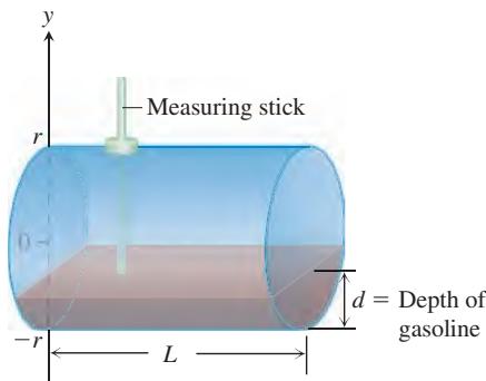
Volume The head of your firm’s accounting department has asked you to find a formula she can use in a computer program to calculate the year-end inventory of gasoline in the company’s tanks. A typical tank is shaped like a right circular cylinder of radius $𝑟$ and length $𝐿$ , mounted horizontally, as shown in the accompanying figure. The data come to the accounting office as depth measurements taken with a vertical measuring stick marked in centimeters.

a. Show, in the notation of the figure, that the volume of gasoline that fills the tank to a depth $𝑑$ is

𝑉 = 2 𝐿 \int - 𝑟 + 𝑑 - 𝑟 \sqrt 𝑟 2 - 𝑦 2 𝑑 𝑦 .

b. Evaluate the integral.

教材插图

What is the largest value that

\int 𝑏 𝑎 \sqrt 𝑥 - 𝑥 2 𝑑 𝑥

can have for any $𝑎$ and $𝑏$ ? Give reasons for your answer.

What is the largest value that

\int 𝑏 𝑎 𝑥 \sqrt 2 𝑥 - 𝑥 2 𝑑 𝑥

can have for any a and b? Give reasons for your answer.

COMPUTER EXPLORATIONS

In Exercises 65 and 66, use a CAS to perform the integrations.

Evaluate the integrals

a. $\int 𝑥 l n 𝑥 𝑑 𝑥$ b. $\int 𝑥 2 l n 𝑥 𝑑 𝑥$ c. $\int 𝑥 3 l n 𝑥 𝑑 𝑥 .$

d. What pattern do you see? Predict the formula for $\int 𝑥 4 l n 𝑥 𝑑 𝑥$ and then see if you are correct by evaluating it with a CAS.

e. What is the formula for $\int 𝑥 𝑛 l n 𝑥 𝑑 𝑥, 𝑛 \geq 1$ ? Check your answer using a CAS.

Evaluate the integrals

a. $\int l n 𝑥 𝑥 2 𝑑 𝑥$

b. $\int l n 𝑥 𝑥 3 𝑑 𝑥$

\int l n 𝑥 𝑥 4 𝑑 𝑥 .

d. What pattern do you see? Predict the formula for

\int l n 𝑥 𝑥 5 𝑑 𝑥

and then see if you are correct by evaluating it with a CAS.

e. What is the formula for

\int l n 𝑥 𝑥 𝑛 𝑑 𝑥, 𝑛 \geq 2 ?

Check your answer using a CAS.

a. Use a CAS to evaluate

\int 𝜋 / 2 0 s i n 𝑛 𝑥 s i n 𝑛 𝑥 + c o s 𝑛 𝑥 𝑑 𝑥,

where n is an arbitrary positive integer. Does your CAS find the result?

b. In succession, find the integral when $𝑛 = 1, 2, 3, 5$ , and 7. Comment on the complexity of the results.

c. Now substitute $𝑥 = (𝜋 / 2) - 𝑢$ and add the new and old integrals. What is the value of

\int 𝜋 / 2 0 s i n 𝑛 𝑥 s i n 𝑛 𝑥 + c o s 𝑛 𝑥 𝑑 𝑥 ?

This exercise illustrates how a little mathematical ingenuity can sometimes solve a problem not immediately amenable to solution by a CAS.

8.7 Numerical Integration

The antiderivatives of some functions, like $s i n (𝑥 2)$ , $1 / l n 𝑥$ , and $\sqrt 1 + 𝑥 4$ , have no elementary formulas. When we cannot find a workable antiderivative for a function f that we have to integrate, we can partition the interval of integration, replace f by a closely fitting polynomial on each subinterval, integrate the polynomials, and add the results to approximate the definite integral of f. This procedure is an example of numerical integration. In this section we start by revisiting the Midpoint Rule, which we studied in Section 5.2. We then study two new methods, the Trapezoidal Rule and Simpson’s Rule. A key goal in our analysis is to control the possible error that is introduced when computing an approximation to an integral.

Approximating Integrals with the Midpoint Rule

In Section 5.2 we introduced the Midpoint Rule to approximate a definite integral over an interval $[𝑎, 𝑏]$ . The rule is based on subdividing $[𝑎, 𝑏]$ into n equal subintervals,

[𝑥 0, 𝑥 1], [𝑥 1, 𝑥 2], \dots, [𝑥 𝑛 - 1, 𝑥 𝑛]

each of width

Δ 𝑥 = 𝑏 - 𝑎 𝑛 .

We then approximate the integral using n rectangles, where the height of the kth rectangle is the value of f at the midpoint $𝑐 𝑘 = (𝑥 𝑘 - 1 + 𝑥 𝑘) / 2$ of the kth subinterval $[𝑥 𝑘 - 1, 𝑥 𝑘]$ .

Midpoint Rule for Approximating a Definite Integral

\int 𝑏 𝑎 𝑓 (𝑥) 𝑑 𝑥 \approx 𝑛 \sum 𝑘 = 1 𝑓 (𝑐 𝑘) (𝑏 - 𝑎 𝑛) = [𝑓 (𝑐 1) + 𝑓 (𝑐 2) + \dots + 𝑓 (𝑐 𝑛)] (𝑏 - 𝑎 𝑛)

with $𝑐 𝑘 = 𝑥 𝑘 - 1 + 𝑥 𝑘 2$ and $𝑥 𝑘 = 𝑎 + 𝑘 (𝑏 - 𝑎 𝑛)$ .

Trapezoidal Approximations

The Trapezoidal Rule for the value of a definite integral is based on approximating the region between a curve and the $𝑥$ -axis with trapezoids instead of rectangles, as in Figure 8.7. It is not necessary for the subdivision points $𝑥 0, 𝑥 1, 𝑥 2, \dots, 𝑥 𝑛$ in the figure to be evenly spaced, but the resulting formula is simpler if they are. We therefore assume that the length of each subinterval is

Δ 𝑥 = 𝑏 - 𝑎 𝑛 .

The length $Δ 𝑥 = (𝑏 - 𝑎) / 𝑛$ is called the step size or mesh size. The area of the trapezoid that lies above the ith subinterval is

Δ 𝑥 (𝑦 𝑖 - 1 + 𝑦 𝑖 2) = Δ 𝑥 2 (𝑦 𝑖 - 1 + 𝑦 𝑖),

教材插图

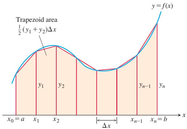
FIGURE 8.7 The Trapezoidal Rule approximates short stretches of the curve $𝑦 = 𝑓 (𝑥)$ with line segments. To approximate the integral of f from a to b, we add the areas of the trapezoids made by vertically joining the ends of the segments to the x-axis.

where $𝑦 𝑖 - 1 = 𝑓 (𝑥 𝑖 - 1)$ and $𝑦 𝑖 = 𝑓 (𝑥 𝑖)$ . (See Figure 8.7.) The area below the curve $𝑦 = 𝑓 (𝑥)$ and above the x-axis is then approximated by adding the areas of all the trapezoids:

𝑇 = 12 (𝑦 0 + 𝑦 1) Δ 𝑥 + 12 (𝑦 1 + 𝑦 2) Δ 𝑥 + \dots + 12 (𝑦 𝑛 - 2 + 𝑦 𝑛 - 1) Δ 𝑥 + 12 (𝑦 𝑛 - 1 + 𝑦 𝑛) Δ 𝑥 = Δ 𝑥 (12 𝑦 0 + 𝑦 1 + 𝑦 2 + \dots + 𝑦 𝑛 - 1 + 12 𝑦 𝑛) = Δ 𝑥 2 (𝑦 0 + 2 𝑦 1 + 2 𝑦 2 + \dots + 2 𝑦 𝑛 - 1 + 𝑦 𝑛),

where

𝑦 0 = 𝑓 (𝑎), 𝑦 1 = 𝑓 (𝑥 1), \dots, 𝑦 𝑛 - 1 = 𝑓 (𝑥 𝑛 - 1), 𝑦 𝑛 = 𝑓 (𝑏) .

The Trapezoidal Rule says: Use T to estimate the integral of f from a to b.

教材插图

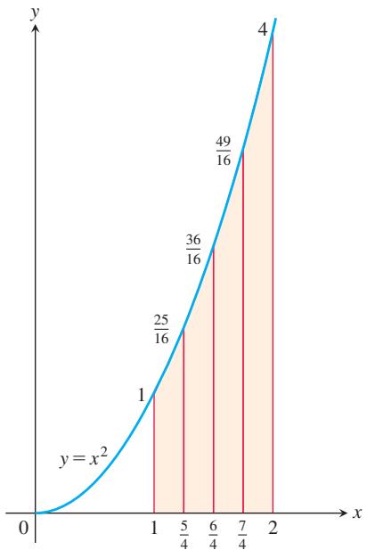
FIGURE 8.8 The trapezoidal approximation of the area under the graph of $𝑦 = 𝑥 2$ from $𝑥 = 1$ to $𝑥 = 2$ is a slight overestimate (Example 1).

TABLE 8.2

x	$𝑦 = 𝑥 2$
1	1
$54$	$2516$
$64$	$3616$
$74$	$4916$
2	4

教材插图

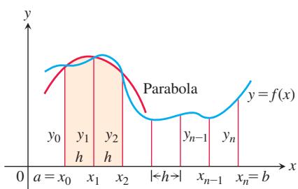
FIGURE 8.9 Simpson’s Rule approximates short stretches of the curve with parabolas.

The Trapezoidal Rule To approximate $\int 𝑏 𝑎 𝑓 (𝑥) 𝑑 𝑥$ , use [ T = \frac{\Delta x}{2}(y_0 + 2y_1 + 2y_2 + \cdots + 2y_{n-1} + y_n). ] The y’s are the values of f at the partition points $𝑥 0 = 𝑎, 𝑥 1 = 𝑎 + Δ 𝑥, 𝑥 2 = 𝑎 + 2 Δ 𝑥, \dots, 𝑥 𝑛 - 1 = 𝑎 + (𝑛 - 1) Δ 𝑥, 𝑥 𝑛 = 𝑏,$ where $Δ 𝑥 = (𝑏 - 𝑎) / 𝑛 .$

EXAMPLE 1 Use the Trapezoidal Rule with n = 4 to estimate $\int 21 𝑥 2 𝑑 𝑥$ . Compare the estimate with the exact value.

Solution Partition [1, 2] into four subintervals of equal length (Figure 8.8). Then evaluate $𝑦 = 𝑥 2$ at each partition point (Table 8.2).

Using these $𝑦$ -values, $𝑛 = 4$ , and $Δ 𝑥 = (2 - 1) / 4 = 1 / 4$ in the Trapezoidal Rule, we have

𝑇 = Δ 𝑥 2 (𝑦 0 + 2 𝑦 1 + 2 𝑦 2 + 2 𝑦 3 + 𝑦 4) = 18 (1 + 2 (2516) + 2 (3616) + 2 (4916) + 4) = 7532 = 2 . 3437 5 .

Since the parabola is concave up, the approximating segments lie above the curve, giving each trapezoid slightly more area than the corresponding strip under the curve. The exact value of the integral is

\int 21 𝑥 2 𝑑 𝑥 = 𝑥 3 3] 21 = 83 - 13 = 73 .

The $𝑇$ approximation overestimates the integral by about half a percent of its true value of 7/3. The percentage error is $(2.34375 - 7 / 3) / (7 / 3) \approx 0.00446$ , or $0.446 %$ .

Simpson’s Rule: Approximations Using Parabolas

Another rule for approximating the definite integral of a continuous function results from using parabolas instead of the straight-line segments that produced trapezoids. As before, we partition the interval $[𝑎, 𝑏]$ into n subintervals of equal length $ℎ = Δ 𝑥 = (𝑏 - 𝑎) / 𝑛$ , but this time we require that n be an even number. On each consecutive pair of intervals we approximate the curve $𝑦 = 𝑓 (𝑥) \geq 0$ by a parabola, as shown in Figure 8.9. A typical parabola passes through three consecutive points $(𝑥 𝑖 - 1, 𝑦 𝑖 - 1)$ , $(𝑥 𝑖, 𝑦 𝑖)$ , and $(𝑥 𝑖 + 1, 𝑦 𝑖 + 1)$ on the curve.

Let’s calculate the shaded area beneath a parabola passing through three consecutive points. To simplify our calculations, we first take the case where $𝑥 0 = - ℎ$ , $𝑥 1 = 0$ , and $𝑥 2 = ℎ$ (Figure 8.10), where $ℎ = Δ 𝑥 = (𝑏 - 𝑎) / 𝑛$ . The area under the parabola will be the same if we shift the $𝑦$ -axis to the left or right. The parabola has an equation of the form

𝑦 = 𝐴 𝑥 2 + 𝐵 𝑥 + 𝐶,

教材插图

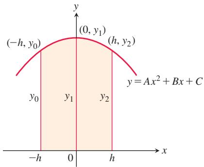
FIGURE 8.10 By integrating from -h to h, we find the shaded area to be

ℎ 3 (𝑦 0 + 4 𝑦 1 + 𝑦 2) .

so the area under it from x = -h to x = h is

𝐴 𝑝 = \int ℎ - ℎ (𝐴 𝑥 2 + 𝐵 𝑥 + 𝐶) 𝑑 𝑥 = [𝐴 𝑥 3 3 + 𝐵 𝑥 2 2 + 𝐶 𝑥] ℎ - ℎ = 2 𝐴 ℎ 3 3 + 2 𝐶 ℎ = ℎ 3 (2 𝐴 ℎ 2 + 6 𝐶) .

Since the curve passes through the three points $(- ℎ, 𝑦 0), (0, 𝑦 1)$ , and $(ℎ, 𝑦 2)$ , we also have

𝑦 0 = 𝐴 ℎ 2 - 𝐵 ℎ + 𝐶, 𝑦 1 = 𝐶, 𝑦 2 = 𝐴 ℎ 2 + 𝐵 ℎ + 𝐶 .

After some algebraic manipulation, we find that

𝐴 𝑝 = ℎ 3 (𝑦 0 + 4 𝑦 1 + 𝑦 2) .

Now shifting the parabola horizontally to its shaded position in Figure 8.9 does not change the area under it. Thus the area under the parabola through $(𝑥 0, 𝑦 0)$ , $(𝑥 1, 𝑦 1)$ , and $(𝑥 2, 𝑦 2)$ in Figure 8.9 is still

ℎ 3 (𝑦 0 + 4 𝑦 1 + 𝑦 2) .

Similarly, the area under the parabola through the points $(𝑥 2, 𝑦 2)$ , $(𝑥 3, 𝑦 3)$ , and $(𝑥 4, 𝑦 4)$ is

ℎ 3 (𝑦 2 + 4 𝑦 3 + 𝑦 4) .

Computing the areas under all the parabolas and adding the results give the approximation

HISTORICAL BIOGRAPHY

To know more, visit the companion Website.

Thomas Simpson (1720–1761)

Simpson was a successful text writer and did most of his research on probability. Simpson’s rule to approximate definite integrals was developed before he was born. It is another of history’s beautiful quirks that one of the ablest mathematicians of the 18th century is remembered not for his own work but for a rule that was never his, that he never claimed, and that bears his name only because he happened to mention it in one of his books.

\int 𝑏 𝑎 𝑓 (𝑥) 𝑑 𝑥 \approx ℎ 3 (𝑦 0 + 4 𝑦 1 + 𝑦 2) + ℎ 3 (𝑦 2 + 4 𝑦 3 + 𝑦 4) + \dots + ℎ 3 (𝑦 𝑛 - 2 + 4 𝑦 𝑛 - 1 + 𝑦 𝑛) = ℎ 3 (𝑦 0 + 4 𝑦 1 + 2 𝑦 2 + 4 𝑦 3 + 2 𝑦 4 + \dots + 2 𝑦 𝑛 - 2 + 4 𝑦 𝑛 - 1 + 𝑦 𝑛) .

The result is known as Simpson’s Rule. The function need not be positive, as in our derivation, but the number $𝑛$ of subintervals must be even for us to apply the rule because each parabolic arc uses two subintervals.

Simpson’s Rule

To approximate $\int 𝑏 𝑎 𝑓 (𝑥) 𝑑 𝑥$ , use

𝑆 = Δ 𝑥 3 (𝑦 0 + 4 𝑦 1 + 2 𝑦 2 + 4 𝑦 3 + \dots + 2 𝑦 𝑛 - 2 + 4 𝑦 𝑛 - 1 + 𝑦 𝑛) .

The $𝑦$ ‘s are the values of $𝑓$ at the partition points

𝑥 0 = 𝑎, 𝑥 1 = 𝑎 + Δ 𝑥, 𝑥 2 = 𝑎 + 2 Δ 𝑥, \dots, 𝑥 𝑛 - 1 = 𝑎 + (𝑛 - 1) Δ 𝑥, 𝑥 𝑛 = 𝑏 .

The number $𝑛$ is even, and $Δ 𝑥 = (𝑏 - 𝑎) / 𝑛$ .

Note the pattern of the coefficients in the above rule: 1, 4, 2, 4, 2, 4, 2, …, 4, 1.

EXAMPLE 2 Use Simpson’s Rule with $𝑛 = 4$ to approximate $\int 20 5 𝑥 4 𝑑 𝑥$ .

TABLE 8.3

x	$𝑦 = 5 𝑥 4$
0	0
$12$	$516$
1	5
$32$	$40516$
2	80

Solution Partition [0, 2] into four subintervals and evaluate $𝑦 = 5 𝑥 4$ at the partition points (Table 8.3). Then apply Simpson’s Rule with $𝑛 = 4$ and $Δ 𝑥 = 1 / 2$ :

𝑆 = Δ 𝑥 3 (𝑦 0 + 4 𝑦 1 + 2 𝑦 2 + 4 𝑦 3 + 𝑦 4) = 16 (0 + 4 (516) + 2 (5) + 4 (40516) + 80) = 32112 .

This estimate differs from the exact value (32) by only 1/12, a percentage error of less than three-tenths of one percent, and this was with just four subintervals.

Error Analysis

Whenever we use an approximation technique, we must consider how accurate the approximation might be. The following theorem gives formulas for estimating the errors when using the Midpoint Rule, the Trapezoidal Rule, and Simpson’s Rule. The error is the difference between the approximation obtained by using the rule and the actual value of the definite integral $\int 𝑏 𝑎 𝑓 (𝑥) 𝑑 𝑥$ .

THEOREM 1—Error Estimates in the Midpoint, Trapezoidal, and Simpson’s Rules

If $𝑓 ″$ is continuous and M is any upper bound for the values of $| 𝑓 ″ |$ on [a, b], then the error $𝐸 𝑀$ in the Midpoint Rule approximation of the integral of f from a to b for n steps satisfies the inequality

| 𝐸 𝑀 | \leq 𝑀 (𝑏 - 𝑎) 3 24 𝑛 2 . M i d p o i n t R u l e

If $𝑓 ″$ is continuous and M is any upper bound for the values of $| 𝑓 ″ |$ on [a, b], then the error $𝐸 𝑇$ in the Trapezoidal Rule approximation of the integral of f from a to b for n steps satisfies the inequality

| 𝐸 𝑇 | \leq 𝑀 (𝑏 - 𝑎) 3 12 𝑛 2 . T r a p e z o i d a l R u l e

If $𝑓 (4)$ is continuous and $𝑀$ is any upper bound for the values of $| 𝑓 (4) |$ on $[𝑎, 𝑏]$ , then the error $𝐸 𝑆$ in the Simpson’s Rule approximation of the integral of $𝑓$ from $𝑎$ to $𝑏$ for $𝑛$ steps satisfies the inequality

| 𝐸 𝑆 | \leq 𝑀 (𝑏 - 𝑎) 5 180 𝑛 4 . S i m p s o n' s R u l e

To give an idea of why Theorem 1 is true in the case of the Trapezoidal Rule, we begin with a result which says that if $𝑓 ″$ is continuous on the interval $[𝑎, 𝑏]$ , then

\int 𝑏 𝑎 𝑓 (𝑥) 𝑑 𝑥 = 𝑇 - 𝑏 - 𝑎 12 \cdot 𝑓'' (𝑐) (Δ 𝑥) 2

for some number $𝑐$ between $𝑎$ and $𝑏$ . This result follows from Taylor’s Remainder Theorem, which we discuss in Theorem 24 of Section 9.9. It follows that as $Δ 𝑥$ approaches zero, the error defined by

𝐸 𝑇 = - 𝑏 - 𝑎 12 \cdot 𝑓'' (𝑐) (Δ 𝑥) 2

approaches zero at the rate of the square of $Δ 𝑥$ .

The inequality

| 𝐸 𝑇 | \leq 𝑏 - 𝑎 12 m a x | 𝑓'' (𝑥) | (Δ 𝑥) 2,

where “max” refers to the maximum of $| 𝑓 ″ (𝑥) |$ over the interval $[𝑎, 𝑏]$ , gives an upper bound for the magnitude of the error. In practice, we usually cannot find the exact value of $m a x | 𝑓 ″ (𝑥) |$ and have to estimate an upper bound or “worst case” value for it instead. If M is any upper bound for the values of $| 𝑓 ″ (𝑥) |$ on $[𝑎, 𝑏]$ , so that $| 𝑓 ″ (𝑥) | \leq 𝑀$ for every x in $[𝑎, 𝑏]$ , then

| 𝐸 𝑇 | \leq 𝑏 - 𝑎 12 𝑀 (Δ 𝑥) 2 .

If we substitute $(𝑏 - 𝑎) / 𝑛$ for $Δ 𝑥$ , we get

| 𝐸 𝑇 | \leq 𝑀 (𝑏 - 𝑎) 3 12 𝑛 2 .

The upper bound for the error in the Midpoint Rule,

| 𝐸 𝑀 | \leq 𝑀 (𝑏 - 𝑎) 3 24 𝑛 2,

is based on a similar argument. Taylor’s Remainder Theorem implies that the Midpoint Rule approximation and the definite integral differ by at most

| 𝑓'' (𝑐) | (𝑏 - 𝑎) 3 24 𝑛 2

for some $𝑐 \in [𝑎, 𝑏]$ . Taking $𝑀$ to be at least as large as the maximum of $| 𝑓 ″ (𝑐) |$ on $[𝑎, 𝑏]$ , we obtain the error bound in Theorem 1. Note that this is half as large as the error bound for the Trapezoidal Rule. This does not mean that the Midpoint Rule is always more accurate than the Trapezoidal Rule, but rather that the largest possible error that might occur is only half as large as the largest possible error for the Trapezoidal Rule.

To estimate the error in Simpson’s Rule, we start with a result, again following from Taylor’s Remainder Theorem, that says that if the fourth derivative $𝑓 (4)$ is continuous, then

\int 𝑏 𝑎 𝑓 (𝑥) 𝑑 𝑥 = 𝑆 - 𝑏 - 𝑎 180 \cdot 𝑓 (4) (𝑐) (Δ 𝑥) 4

for some point c between a and b. Thus, as $Δ 𝑥$ approaches zero, the error,

𝐸 𝑆 = - 𝑏 - 𝑎 180 \cdot 𝑓 (4) (𝑐) (Δ 𝑥) 4,

approaches zero as the fourth power of $Δ 𝑥$ . (This helps to explain why Simpson’s Rule is likely to give better results than the Trapezoidal Rule.)

The inequality

| 𝐸 𝑆 | \leq 𝑏 - 𝑎 180 m a x ∣ 𝑓 (4) (𝑥) ∣ (Δ 𝑥) 4,

where “max” refers to the maximum of $| 𝑓 (4) (𝑥) |$ over the interval [a, b], gives an upper bound for the magnitude of the error. As with $m a x | 𝑓 ″ |$ in the error formula for the Trapezoidal Rule, we usually cannot find the exact value of $m a x | 𝑓 (4) (𝑥) |$ and have to replace it with an upper bound. If M is any upper bound for the values of $| 𝑓 (4) (𝑥) |$ on [a, b], then

| 𝐸 𝑆 | \leq 𝑏 - 𝑎 180 𝑀 (Δ 𝑥) 4 .

Substituting $(𝑏 - 𝑎) / 𝑛$ for $Δ 𝑥$ in this last expression gives

| 𝐸 𝑠 | \leq 𝑀 (𝑏 - 𝑎) 5 180 𝑛 4 .

You might wonder why we don’t just take $𝑀$ to be the maximum value of $| 𝑓 ″ (𝑥) |$ on $[𝑎, 𝑏]$ for the first two rules, or the maximum value of $| 𝑓 (4) (𝑥) |$ for Simpson’s Rule. The reason is that sometimes this maximum is hard to compute, while a less accurate upper bound is easily found. We can certainly set $𝑀$ to the maximum value if we can compute it.

EXAMPLE 3 Find an upper bound for the error in estimating $\int 20 5 𝑥 4 𝑑 𝑥$ using Simpson’s Rule with $𝑛 = 4$ (Example 2).

Solution To estimate the error, we first find an upper bound M for the magnitude of the fourth derivative of $𝑓 (𝑥) = 5 𝑥 4$ on the interval $0 \leq 𝑥 \leq 2$ . Since the fourth derivative has the constant value $𝑓 (4) (𝑥) = 120$ , we take M = 120. With b - a = 2 and n = 4, the error estimate for Simpson’s Rule gives

| 𝐸 𝑠 | \leq 𝑀 (𝑏 - 𝑎) 5 180 𝑛 4 = 120 (2) 5 180 \cdot 44 = 112 .

This estimate is consistent with the result of Example 2.

Theorem 1 can also be used to estimate the number of subintervals required when using the Trapezoidal or Simpson’s Rule if we specify a certain tolerance for the error.

EXAMPLE 4 Estimate the minimum number of subintervals needed to approximate the integral in Example 3 using Simpson’s Rule with an error of magnitude less than $10 - 4$ .

Solution Using the inequality in Theorem 1, if we choose the number of subintervals $𝑛$ to satisfy

𝑀 (𝑏 - 𝑎) 5 180 𝑛 4 < 1 0 - 4,

then the error $𝐸 𝑆$ in Simpson’s Rule satisfies $| 𝐸 𝑆 | < 10 - 4$ , as required.

From the solution in Example 3, we have $𝑀 = 120$ and $𝑏 - 𝑎 = 2$ , so we want $𝑛$ to satisfy

120 (2) 5 180 𝑛 4 < 1104,

or, equivalently,

𝑛 4 > 64 \cdot 104 3 .

It follows that

𝑛 > 10 (643) 1 / 4 \approx 2 1 . 5 .

Since $𝑛$ must be even in Simpson’s Rule, we estimate the minimum number of subintervals required for the error tolerance to be $𝑛 = 22$ .

EXAMPLE 5 As we saw in Chapter 7, the value of $l n 2$ can be calculated from the integral

l n 2 = \int 21 1 𝑥 𝑑 𝑥 .

Table 8.4 shows values of $𝑇$ and $𝑆$ for approximations of $\int 21 (1 / 𝑥) 𝑑 𝑥$ using various values of $𝑛$ . Notice how Simpson’s Rule dramatically improves over the Trapezoidal Rule.

TABLE 8.4 Trapezoidal Rule approximations $(𝑇 𝑛)$ and Simpson’s Rule approximations $(𝑆 𝑛)$ of $l n 2 = \int 21 (1 / 𝑥) 𝑑 𝑥$

n	$𝑇 𝑛$	\|Error\| less than...	$𝑆 𝑛$	\|Error\| less than...
10	0.6937714032	0.0006242227	0.6931502307	0.0000030502
20	0.6933033818	0.0001562013	0.6931473747	0.0000001942
30	0.6932166154	0.0000694349	0.6931472190	0.0000000385
40	0.6931862400	0.0000390595	0.6931471927	0.0000000122
50	0.6931721793	0.0000249988	0.6931471856	0.0000000050
100	0.6931534305	0.0000062500	0.6931471809	0.0000000004

In particular, notice that when we double the value of n (thereby halving the value of $ℎ = Δ 𝑥$ ), the T error is divided by 2 squared, whereas the S error is divided by 2 to the fourth.

This has a dramatic effect as $Δ 𝑥 = (2 - 1) / 𝑛$ gets very small. The Simpson approximation for n = 50 rounds accurately to seven places and for n = 100 is accurate to nine decimal places (billionths)!

If $𝑓 (𝑥)$ is a polynomial of degree less than 4, then its fourth derivative is zero, and

𝐸 𝑆 = - 𝑏 - 𝑎 180 𝑓 (4) (𝑐) (Δ 𝑥) 4 = - 𝑏 - 𝑎 180 (0) (Δ 𝑥) 4 = 0 .

Thus, there will be no error in the Simpson approximation of any integral of $𝑓$ . In other words, if $𝑓$ is a constant, a linear function, or a quadratic or cubic polynomial, Simpson’s Rule will give the value of any integral of $𝑓$ exactly, whatever the number of subdivisions. Similarly, if $𝑓$ is a constant or a linear function, then its second derivative is zero, and

𝐸 𝑇 = - 𝑏 - 𝑎 12 𝑓'' (𝑐) (Δ 𝑥) 2 = - 𝑏 - 𝑎 12 (0) (Δ 𝑥) 2 = 0 .

The Trapezoidal Rule will therefore give the exact value of any integral of $𝑓$ . This is no surprise, for the trapezoids fit the graph perfectly.

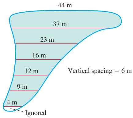
Although decreasing the step size $Δ 𝑥$ reduces the error in the Simpson and Trapezoidal approximations in theory, it may fail to do so in practice. When $Δ 𝑥$ is very small, say $Δ 𝑥 = 10 - 8$ , computer or calculator round-off errors in the arithmetic required to evaluate S and T may accumulate to such an extent that the error formulas no longer describe what is going on. Shrinking $Δ 𝑥$ below a certain size can actually make things worse. You should consult a text on numerical analysis for more sophisticated methods if you are having problems with round-off error using the rules discussed in this section.

教材插图

FIGURE 8.11 The dimensions of the swamp in Example 6.

EXAMPLE 6 A town wants to drain and fill a polluted swamp (Figure 8.11). The swamp averages 1.5 m deep. About how many cubic meters of dirt will it take to fill the area after the swamp is drained?

Solution To calculate the volume of the swamp, we estimate the surface area and multiply by 1.5. To estimate the area, we use Simpson’s Rule with $Δ 𝑥 = 6 m$ , and the $𝑦$ s equal to the distances measured across the swamp, as shown in Figure 8.11.

𝑆 = Δ 𝑥 3 (𝑦 0 + 4 𝑦 1 + 2 𝑦 2 + 4 𝑦 3 + 2 𝑦 4 + 4 𝑦 5 + 𝑦 6) = 63 (44 + 148 + 46 + 64 + 24 + 36 + 4) = 732

The volume is about (732)(1.5) = 1098 m $4$ .

EXERCISES 8.7

For some exercises, a calculator may be helpful for expressing answers in decimal form.

Estimating Definite Integrals

The instructions for the integrals in Exercises 1–10 have three parts, one for the Midpoint Rule, one for the Trapezoidal Rule, and one for Simpson’s Rule.

I. Using the Midpoint Rule

a. Estimate the integral with $𝑛 = 4$ steps and find an upper bound for $| 𝐸 𝑀 |$ .

b. Evaluate the integral directly and find $| 𝐸 𝑀 |$ .

c. Use the formula $(| 𝐸 𝑀 | / (t r u e v a l u e)) \times 100$ to express $| 𝐸 𝑀 |$ as a percentage of the integral’s true value.

II. Using the Trapezoidal Rule

a. Estimate the integral with $𝑛 = 4$ steps and find an upper bound for $| 𝐸 𝑇 |$ .

b. Evaluate the integral directly and find $| 𝐸 𝑇 |$ .

c. Use the formula $(| 𝐸 𝑇 | / (t r u e v a l u e)) \times 100$ to express $| 𝐸 𝑇 |$ as a percentage of the integral’s true value.

III. Using Simpson’s Rule

a. Estimate the integral with $𝑛 = 4$ steps and find an upper bound for $| 𝐸 𝑆 |$ .

b. Evaluate the integral directly and find $| 𝐸 𝑆 |$ .

c. Use the formula $(| 𝐸 𝑆 | / (t r u e v a l u e)) \times 100$ to express $| 𝐸 𝑆 |$ as a percentage of the integral’s true value.

$\int 21 𝑥 𝑑 𝑥$
$\int 31 (2 𝑥 - 1) 𝑑 𝑥$
$\int 1 - 1 (𝑥 2 + 1) 𝑑 𝑥$
$\int 0 - 2 (𝑥 2 - 1) 𝑑 𝑥$

\int 21 1 𝑠 2 𝑑 𝑠

$\int 20 (𝑡 3 + 𝑡) 𝑑 𝑡$
$\int 1 - 1 (𝑡 3 + 1) 𝑑 𝑡$
$\int 42 1 (𝑠 - 1) 2 𝑑 𝑠$

\int 𝜋 0 s i n 𝑡 𝑑 𝑡

\int 10 s i n 𝜋 𝑡 𝑑 𝑡

Estimating the Number of Subintervals

In Exercises 11–22, estimate the minimum number of subintervals needed to approximate the integrals with an error of magnitude less than $10 - 4$ by (a) the Trapezoidal Rule and (b) Simpson’s Rule. (The integrals in Exercises 11–18 are the integrals from Exercises 1–8.)

$\int 21 𝑥 𝑑 𝑥$
$\int 31 (2 𝑥 - 1) 𝑑 𝑥$
$\int 1 - 1 (𝑥 2 + 1) 𝑑 𝑥$
$\int 0 - 2 (𝑥 2 - 1) 𝑑 𝑥$
$\int 20 (𝑡 3 + 𝑡) 𝑑 𝑡$
$\int 1 - 1 (𝑡 3 + 1) 𝑑 𝑡$
$\int 21 1 𝑠 2 𝑑 𝑠$
$\int 42 1 (𝑠 - 1) 2 𝑑 𝑠$
$\int 30 \sqrt 𝑥 + 1 𝑑 𝑥$
$\int 30 1 \sqrt 𝑥 + 1 𝑑 𝑥$
$\int 20 s i n (𝑥 + 1) 𝑑 𝑥$
$\int 1 - 1 c o s (𝑥 + 𝜋) 𝑑 𝑥$

Estimates with Numerical Data

Volume of water in a swimming pool A rectangular swimming pool is 5 m wide and 10 m long. The accompanying table shows the depth $ℎ (𝑥)$ of the water at 1-m intervals from one end of the pool to the other. Estimate the volume of water in the pool using the Trapezoidal Rule with n = 10 applied to the integral

𝑉 = \int 100 5 \cdot ℎ (𝑥) 𝑑 𝑥 .

Position (m) x	Depth (m) h(x)	Position (m) x	Depth (m) h(x)
0	1.20	6	2.30
1	1.64	7	2.38
2	1.82	8	2.46
3	1.98	9	2.54
4	2.10	10	2.60
5	2.20

Distance traveled The accompanying table shows time-to-speed data for a car accelerating from rest to 130 km/h. How far had the car traveled by the time it reached this speed? (Use trapezoids to estimate the area under the velocity curve, but be careful: The time intervals vary in length.)

Speed change	Time (s)
Zero to 30 km/h	2.2
40 km/h	3.2
50 km/h	4.5
60 km/h	5.9
70 km/h	7.8
80 km/h	10.2
90 km/h	12.7
100 km/h	16.0
110 km/h	20.6
120 km/h	26.2
130 km/h	37.1

Wing design The design of a new airplane requires a gasoline tank of constant cross-sectional area in each wing. A scale drawing of a cross-section is shown here. The tank must hold 2000 kg of gasoline, which has a density of $673 k g / m 3$ . Estimate the length of the tank by Simpson’s Rule.

教材插图

𝑦 3 = 0 . 65 r

𝑦 4 = 0 . 7

𝑦 5 = 𝑦 6 = 0 . 75

Oil consumption on Pathfinder Island A diesel generator runs continuously, consuming oil at a gradually increasing rate until it must be temporarily shut down to have the filters replaced. Use the Trapezoidal Rule to estimate the amount of oil consumed by the generator during that week.

Day	Oil consumption rate (liters/hour)
Sun	0.019
Mon	0.020
Tue	0.021
Wed	0.023
Thu	0.025
Fri	0.028
Sat	0.031
Sun	0.035

Theory and Examples

Usable values of the sine-integral function The sine-integral function,

S i (𝑥) = \int 𝑥 0 s i n 𝑡 𝑡 𝑑 𝑡, " S i n e i n t e g r a l o f 𝑥 "

is one of the many functions in engineering whose formulas cannot be simplified. There is no elementary formula for the anti-derivative of $(s i n 𝑡) / 𝑡$ . The values of $S i (𝑥)$ , however, are readily estimated by numerical integration.

Although the notation does not show it explicitly, the function being integrated is

𝑓 (𝑡) = {s i n 𝑡 𝑡, 𝑡 \neq 0 1, 𝑡 = 0,

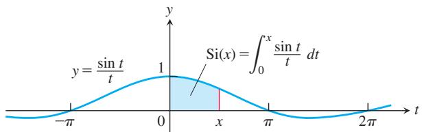
the continuous extension of $(s i n 𝑡) / 𝑡$ to the interval $[0, 𝑥]$ . The function has derivatives of all orders at every point of its domain. Its graph is smooth, and you can expect good results from Simpson’s Rule.

教材插图

a. Use the fact that $| 𝑓 (4) | \leq 1$ on $[0, 𝜋 / 2]$ to give an upper bound for the error that will occur if

S i (𝜋 2) = \int 𝜋 / 2 0 s i n 𝑡 𝑡 𝑑 𝑡

is estimated by Simpson’s Rule with $𝑛 = 4$ .

b. Estimate $S i (𝜋 / 2)$ by Simpson’s Rule with $𝑛 = 4$ .

c. Express the error bound you found in part (a) as a percentage of the value you found in part (b).

The error function The error function,

e r f (𝑥) = 2 \sqrt 𝜋 \int 𝑥 0 𝑒 - 𝑡 2 𝑑 𝑡,

which is important in probability and in the theories of heat flow and signal transmission, must be evaluated numerically because there is no elementary expression for the antiderivative of $𝑒 - 𝑡 2$ .

a. Use Simpson’s Rule with $𝑛 = 10$ to estimate erf (1).

b. In [0, 1],

∣ 𝑑 4 𝑑 𝑡 4 (𝑒 - 𝑡 2) ∣ \leq 1 2 .

Give an upper bound for the magnitude of the error of the estimate in part (a).

Prove that the sum T in the Trapezoidal Rule for $\int 𝑏 𝑎 𝑓 (𝑥) 𝑑 𝑥$ is a Riemann sum for f continuous on [a, b]. (Hint: Use the Intermediate Value Theorem to show the existence of $𝑐 𝑘$ in the subinterval $[𝑥 𝑘 - 1, 𝑥 𝑘]$ satisfying $𝑓 (𝑐 𝑘) = (𝑓 (𝑥 𝑘 - 1) + 𝑓 (𝑥 𝑘)) / 2$ .)
Prove that the sum $𝑆$ in Simpson’s Rule for $\int 𝑏 𝑎 𝑓 (𝑥) 𝑑 𝑥$ is a Riemann sum for $𝑓$ continuous on $[𝑎, 𝑏]$ . (See Exercise 29.)
Elliptic integrals The length of the ellipse

𝑥 2 𝑎 2 + 𝑦 2 𝑏 2 = 1

turns out to be

L e n g t h = 4 𝑎 \int 𝜋 / 2 0 \sqrt 1 - 𝑒 2 c o s 2 𝑡 𝑑 𝑡,

where $𝑒 = \sqrt 𝑎 2 - 𝑏 2 / 𝑎$ is the ellipse’s eccentricity. The integral in this formula, called an elliptic integral, is nonelementary except when $𝑒 = 0$ or 1.

a. Use the Trapezoidal Rule with $𝑛 = 10$ to estimate the length of the ellipse when $𝑎 = 1$ and $𝑒 = 1 / 2$ .

b. Use the fact that the absolute value of the second derivative of $𝑓 (𝑡) = \sqrt 1 - 𝑒 2 c o s 2 𝑡$ is less than 1 to find an upper bound for the error in the estimate you obtained in part (a).

Applications

The length of one arch of the curve $𝑦 = s i n 𝑥$ is given by

𝐿 = \int 𝜋 0 \sqrt 1 + c o s 2 𝑥 𝑑 𝑥 .

Estimate $𝐿$ by Simpson’s Rule with $𝑛 = 8$ .

When solving Exercises 33-40, you may need to use a calculator or a computer.

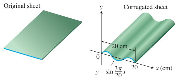
Your metal fabrication company is bidding for a contract to make sheets of corrugated iron roofing like the one shown here. The cross-sections of the corrugated sheets are to conform to the curve

𝑦 = s i n 3 𝜋 20 𝑥, 0 \leq 𝑥 \leq 20 c m .

If the roofing is to be stamped from flat sheets by a process that does not stretch the material, how wide should the original material be? To find out, use numerical integration to approximate the length of the sine curve to two decimal places.

教材插图

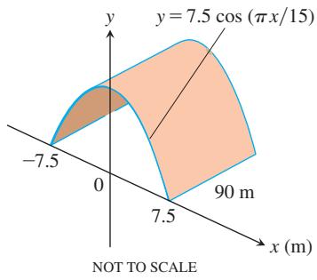
Your engineering firm is bidding for the contract to construct the tunnel shown here. The tunnel is 90 m long and 15 m wide at the base. The cross-section is shaped like one arch of the curve $𝑦 = 7.5 c o s (𝜋 𝑥 / 15)$ . Upon completion, the tunnel’s inside surface (excluding the roadway) will be treated with a waterproof sealer that costs $26.11 per square meter to apply. How much will it cost to apply the sealer? (Hint: Use numerical integration to find the length of the cosine curve.)

教材插图

Find, to two decimal places, the areas of the surfaces generated by revolving the curves in Exercises 35 and 36 about the x-axis.

$𝑦 = s i n 𝑥, 0 \leq 𝑥 \leq 𝜋$
$𝑦 = 𝑥 2 / 4, 0 \leq 𝑥 \leq 2$
Use numerical integration to estimate the value of

a r c s i n 0 . 6 = \int 0 . 6 0 𝑑 𝑥 \sqrt 1 - 𝑥 2 .

For reference, arcsin 0.6 = 0.64350 to five decimal places.

Use numerical integration to estimate the value of

𝜋 = 4 \int 10 1 1 + 𝑥 2 𝑑 𝑥 . 39 . $ 𝐷 𝑟 𝑢 𝑔 𝑎 𝑠 𝑠 𝑖 𝑚 𝑖 𝑙 𝑎 𝑡 𝑖 𝑜 𝑛 𝐴 𝑛 𝑎 𝑣 𝑒 𝑟 𝑎 𝑔 𝑒 𝑎 𝑑 𝑢 𝑙 𝑡 𝑢 𝑛 𝑑 𝑒 𝑟 𝑎 𝑔 𝑒 60 𝑦 𝑒 𝑎 𝑟 𝑠 𝑎 𝑠 𝑠 𝑖 𝑚 𝑖 𝑙 𝑎 𝑡 𝑒 𝑠 𝑎 12 - ℎ 𝑜 𝑢 𝑟 𝑐 𝑜 𝑙 𝑑 𝑚 𝑒 𝑑 𝑖 𝑐 𝑖 𝑛 𝑒 𝑖 𝑛 𝑡 𝑜 ℎ 𝑖 𝑠 𝑜 𝑟 ℎ 𝑒 𝑟 𝑠 𝑦 𝑠 𝑡 𝑒 𝑚 𝑎 𝑡 𝑎 𝑟 𝑎 𝑡 𝑒 𝑚 𝑜 𝑑 𝑒 𝑙 𝑒 𝑑 𝑏 𝑦 $ 𝑑 𝑦 𝑑 𝑡 = 6 - l n (2 𝑡 2 - 3 𝑡 + 3),

where $𝑦$ is measured in milligrams and $𝑡$ is the time in hours since the medication was taken. What amount of medicine is absorbed into a person’s system over a 12-hour period?

Effects of an antihistamine The concentration of an antihistamine in the bloodstream of a healthy adult is modeled by

𝐶 = 1 2 . 5 - 4 l n (𝑡 2 - 3 𝑡 + 4),

where C is measured in grams per liter and t is the time in hours since the medication was taken. What is the average level of concentration in the bloodstream over a 6-hour period?

8.8 Improper Integrals

Up to now, we have required definite integrals to satisfy two properties. First, the domain of integration $[𝑎, 𝑏]$ must be finite. Second, the range of the integrand must be finite on this domain. In practice, we may encounter problems that fail to meet one or both of these conditions. The integral for the area under the curve $𝑦 = (l n 𝑥) / 𝑥 2$ from x = 1 to $𝑥 = \infty$ is an example for which the domain is infinite (Figure 8.12a). The integral for the area under the curve of $𝑦 = 1 / \sqrt 𝑥$ between x = 0 and x = 1 is an example for which the range of the integrand is infinite (Figure 8.12b). In either case, the integrals are said to be improper and are calculated as limits. We will see in Chapter 9 that improper integrals are useful for investigating the convergence of certain infinite series.

教材插图

(b)

教材插图

(a)

教材插图

(b)

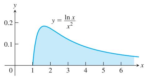
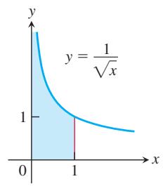
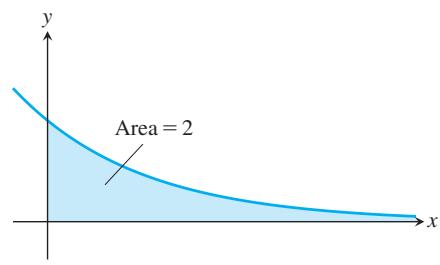
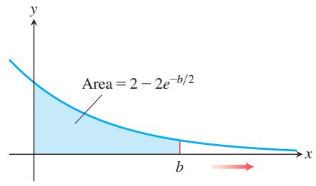
FIGURE 8.13 (a) The area in the first quadrant under the curve $𝑦 = 𝑒 - 𝑥 / 2$ . (b) The area is an improper integral of the first type.

(a)

FIGURE 8.12 Are the areas under these infinite curves finite? We will see that the answer is yes for both curves.

Infinite Limits of Integration

Consider the infinite region (unbounded on the right) that lies under the curve $𝑦 = 𝑒 - 𝑥 / 2$ in the first quadrant (Figure 8.13a). You might think this region has infinite area, but we will see that the value is finite. We assign a value to the area in the following way. First find the area $𝐴 (𝑏)$ of the portion of the region that is bounded on the right by x = b (Figure 8.13b).

𝐴 (𝑏) = \int 𝑏 0 𝑒 - 𝑥 / 2 𝑑 𝑥 = - 2 𝑒 - 𝑥 / 2] 𝑏 0 = - 2 𝑒 - 𝑏 / 2 + 2 = 2 - 2 𝑒 - 𝑏 / 2,

which is a little less than 2. Then find the limit of $𝐴 (𝑏)$ as $𝑏 \to \infty$ .

l i m 𝑏 \to \infty 𝐴 (𝑏) = l i m 𝑏 \to \infty (2 - 2 𝑒 - 𝑏 / 2) = 2

Therefore, the value we assign to the area under the curve from 0 to $\infty$ is

\int \infty 0 𝑒 - 𝑥 / 2 𝑑 𝑥 = l i m 𝑏 \to \infty \int 𝑏 0 𝑒 - 𝑥 / 2 𝑑 𝑥 = 2 .

DEFINITION Integrals with infinite limits of integration are improper integrals of Type I.

If $𝑓 (𝑥)$ is continuous on $[𝑎, \infty)$ , then

$\int \infty 𝑎 𝑓 (𝑥) 𝑑 𝑥 = l i m 𝑏 \to \infty \int 𝑏 𝑎 𝑓 (𝑥) 𝑑 𝑥 .$

If $𝑓 (𝑥)$ is continuous on $(- \infty, 𝑏]$ , then

$\int 𝑏 - \infty 𝑓 (𝑥) 𝑑 𝑥 = l i m 𝑎 \to - \infty \int 𝑏 𝑎 𝑓 (𝑥) 𝑑 𝑥 .$

If $𝑓 (𝑥)$ is continuous on $(- \infty, \infty)$ , then

$\int \infty - \infty 𝑓 (𝑥) 𝑑 𝑥 = \int 𝑐 - \infty 𝑓 (𝑥) 𝑑 𝑥 + \int \infty 𝑐 𝑓 (𝑥) 𝑑 𝑥,$
where $𝑐$ is any real number.

In each case, if the limit exists and is finite, we say that the improper integral converges and that the limit is the value of the improper integral. If the limit fails to exist, the improper integral diverges.

教材插图

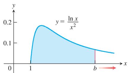
FIGURE 8.14 The area under this curve is an improper integral (Example 1).

HISTORICAL BIOGRAPHY

Lejeune Dirichlet (1805–1859)

Dirichlet, a German mathematician, investigated the solution and equilibrium of systems of differential equations and discovered many results on the convergence of series. In 1855, Dirichlet succeeded Gauss as the professor of mathematics at Göttingen.

To know more, visit the companion Website.

The choice of $𝑐$ in Part 3 of the definition is unimportant. We can evaluate or determine the convergence or divergence of $\int \infty - \infty 𝑓 (𝑥) 𝑑 𝑥$ with any convenient choice.

Any of the integrals in the above definition can be interpreted as an area if $𝑓 \geq 0$ on the interval of integration. For instance, we interpreted the improper integral in Figure 8.13 as an area. In that case, the area has the finite value 2. If $𝑓 \geq 0$ and the improper integral diverges, we say the area under the curve is infinite.

EXAMPLE 1 Is the area under the curve $𝑦 = (l n 𝑥) / 𝑥 2$ from $𝑥 = 1$ to $𝑥 = \infty$ finite? If so, what is its value?

Solution We find the area under the curve from x = 1 to x = b and examine the limit as $𝑏 \to \infty$ . If the limit is finite, we take it to be the area under the curve (Figure 8.14). The area from 1 to b is

\int 𝑏 1 l n 𝑥 𝑥 2 𝑑 𝑥 = [(l n 𝑥) (- 1 𝑥)] 𝑏 1 - \int 𝑏 1 (- 1 𝑥) (1 𝑥) 𝑑 𝑥 I n t e g r a t i o n b y p a r t s w i t h 𝑢 = l n 𝑥, 𝑑 𝑣 = 𝑑 𝑥 / 𝑥 2, 𝑑 𝑢 = 𝑑 𝑥 / 𝑥, 𝑣 = - 1 / 𝑥 = - l n 𝑏 𝑏 - [1 𝑥] 𝑏 1 = - l n 𝑏 𝑏 - 1 𝑏 + 1 .

The limit of the area as $𝑏 \to \infty$ is

∫∞1ln⁡𝑥𝑥2𝑑𝑥=lim𝑏→∞∫𝑏1ln⁡𝑥𝑥2𝑑𝑥=lim𝑏→∞[−ln⁡𝑏𝑏−1𝑏+1]=−[lim𝑏→∞ln⁡𝑏𝑏]−0+1=−[lim𝑏→∞1/𝑏1]+1=0+1=1.(\text{L'Hôpital's Rule})

Thus, the improper integral converges and the area has finite value 1.

EXAMPLE 2 Evaluate

\int \infty - \infty 𝑑 𝑥 1 + 𝑥 2 .

Solution According to Part 3 of the definition, we can choose c = 0 and write

\int \infty - \infty 𝑑 𝑥 1 + 𝑥 2 = \int 0 - \infty 𝑑 𝑥 1 + 𝑥 2 + \int \infty 0 𝑑 𝑥 1 + 𝑥 2 .

Next we evaluate each improper integral on the right side of the equation above.

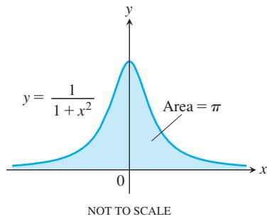
\int 0 - \infty 𝑑 𝑥 1 + 𝑥 2 = l i m 𝑎 \to - \infty \int 0 𝑎 𝑑 𝑥 1 + 𝑥 2 = l i m 𝑎 \to - \infty t a n - 1 𝑥] 0 𝑎 = l i m 𝑎 \to - \infty (t a n - 1 0 - t a n - 1 𝑎) = 0 - (- 𝜋 2) = 𝜋 2

教材插图

FIGURE 8.15 The area under this curve is finite (Example 2).

Thus,

\int \infty 0 𝑑 𝑥 1 + 𝑥 2 = l i m 𝑏 \to \infty \int 𝑏 0 𝑑 𝑥 1 + 𝑥 2 = l i m 𝑏 \to \infty t a n - 1 𝑥] 𝑏 0 = l i m 𝑏 \to \infty (t a n - 1 𝑏 - t a n - 1 0) = 𝜋 2 - 0 = 𝜋 2

\int \infty - \infty 𝑑 𝑥 1 + 𝑥 2 = 𝜋 2 + 𝜋 2 = 𝜋 .

Since $1 / (1 + 𝑥 2) > 0$ , the improper integral can be interpreted as the (finite) area beneath the curve and above the x-axis (Figure 8.15).

The Integral $\int \infty 1 𝑑 𝑥 𝑥 𝑝$

The function y = 1/x is the boundary between the convergent and divergent improper integrals with integrands of the form $𝑦 = 1 / 𝑥 𝑝$ . As the next example shows, the improper integral converges if p > 1 and diverges if $𝑝 \leq 1$ .

EXAMPLE 3 For what values of p does the integral $\int \infty 1 𝑑 𝑥 / 𝑥 𝑝$ converge? When the integral does converge, what is its value?

Solution If $𝑝 \neq 1$ , then

\int 𝑏 1 𝑑 𝑥 𝑥 𝑝 = 𝑥 - 𝑝 + 1 - 𝑝 + 1] 𝑏 1 = (1 1 - 𝑝) (𝑏 - 𝑝 + 1 - 1) = (1 1 - 𝑝) (1 𝑏 𝑝 - 1 - 1) .

Thus,

\int \infty 1 𝑑 𝑥 𝑥 𝑝 = l i m 𝑏 \to \infty \int 𝑏 1 𝑑 𝑥 𝑥 𝑝 = l i m 𝑏 \to \infty [(1 1 - 𝑝) (1 𝑏 𝑝 - 1 - 1)] = {1 𝑝 - 1, 𝑝 > 1 \infty, 𝑝 < 1

because

l i m 𝑏 \to \infty 1 𝑏 𝑝 - 1 = {0, 𝑝 > 1 \infty, 𝑝 < 1 .

Therefore, the integral converges to the value $1 / (𝑝 - 1)$ if $𝑝 > 1$ , and it diverges if $𝑝 < 1$ . If $𝑝 = 1$ , the integral also diverges:

\int \infty 1 𝑑 𝑥 𝑥 𝑝 = \int \infty 1 𝑑 𝑥 𝑥 = l i m 𝑏 \to \infty \int 𝑏 1 𝑑 𝑥 𝑥 = l i m 𝑏 \to \infty [l n | 𝑥 |] 𝑏 1 = l i m 𝑏 \to \infty (l n 𝑏 - l n 1) = \infty .

教材插图

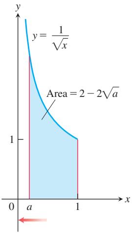
FIGURE 8.16 The area under this curve is an example of an improper integral of the second kind.

Integrands with Vertical Asymptotes

Another type of improper integral arises when the integrand has a vertical asymptote—an infinite discontinuity—at a limit of integration or at some point between the limits of integration. If the integrand f is positive over the interval of integration, we can again interpret the improper integral as the area under the graph of f and above the x-axis between the limits of integration.

Consider the region in the first quadrant that lies under the curve $𝑦 = 1 / \sqrt 𝑥$ from $𝑥 = 0$ to $𝑥 = 1$ (Figure 8.12b). First we find the area of the portion from $𝑎$ to 1 (Figure 8.16):

\int 1 𝑎 𝑑 𝑥 \sqrt 𝑥 = 2 \sqrt 𝑥 ∣ 1 𝑎 = 2 - 2 \sqrt 𝑎 .

Then we find the limit of this area as $𝑎 \to 0 +$ :

l i m 𝑎 \to 0 + \int 1 𝑎 𝑑 𝑥 \sqrt 𝑥 = l i m 𝑎 \to 0 + (2 - 2 \sqrt 𝑎) = 2 .

Therefore, the area under the curve from 0 to 1 is finite and is defined to be

\int 10 𝑑 𝑥 \sqrt 𝑥 = l i m 𝑎 \to 0 + \int 1 𝑎 𝑑 𝑥 \sqrt 𝑥 = 2 .

DEFINITION Integrals of functions that become infinite at a point within the interval of integration are improper integrals of Type II.

If $𝑓 (𝑥)$ is continuous on $(𝑎, 𝑏]$ and discontinuous at a, then

$\int 𝑏 𝑎 𝑓 (𝑥) 𝑑 𝑥 = l i m 𝑐 \to 𝑎 + \int 𝑏 𝑐 𝑓 (𝑥) 𝑑 𝑥 .$

If $𝑓 (𝑥)$ is continuous on $[𝑎, 𝑏)$ and discontinuous at b, then

$\int 𝑏 𝑎 𝑓 (𝑥) 𝑑 𝑥 = l i m 𝑐 \to 𝑏 - \int 𝑐 𝑎 𝑓 (𝑥) 𝑑 𝑥 .$

If $𝑓 (𝑥)$ is discontinuous at $𝑐$ , where $𝑎 < 𝑐 < 𝑏$ , and continuous on $[𝑎, 𝑐) \cup (𝑐, 𝑏]$ , then

$\int 𝑏 𝑎 𝑓 (𝑥) 𝑑 𝑥 = \int 𝑐 𝑎 𝑓 (𝑥) 𝑑 𝑥 + \int 𝑏 𝑐 𝑓 (𝑥) 𝑑 𝑥 .$

In each case, if the limit exists and is finite, we say that the improper integral converges and that the limit is the value of the improper integral. If the limit does not exist, the integral diverges.

In Part 3 of the definition, the integral on the left side of the equation converges if both integrals on the right side converge; otherwise, it diverges.

EXAMPLE 4 Investigate the convergence of

\int 10 1 1 - 𝑥 𝑑 𝑥 .

教材插图

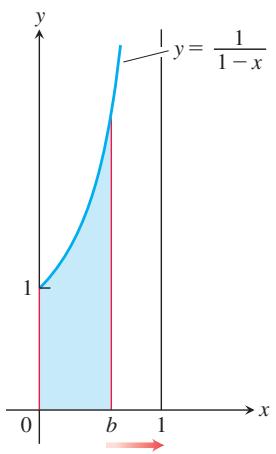
FIGURE 8.17 The area beneath the curve and above the x-axis for $[0, 1)$ is not a real number (Example 4).

教材插图

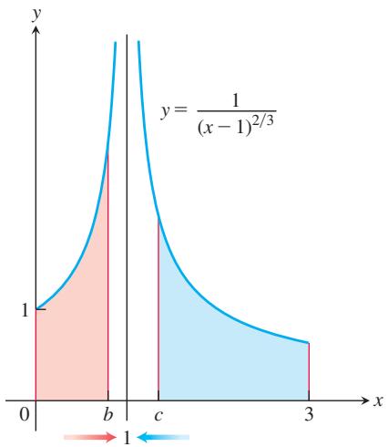
FIGURE 8.18 Example 5 shows that the area under the curve exists (so it is a real number).

Solution The integrand $𝑓 (𝑥) = 1 / (1 - 𝑥)$ is continuous on [0, 1) but is discontinuous at x = 1 and becomes infinite as $𝑥 \to 1 -$ (Figure 8.17). We evaluate the integral as

l i m 𝑏 \to 1 - \int 𝑏 0 1 1 - 𝑥 𝑑 𝑥 = l i m 𝑏 \to 1 - [- l n | 1 - 𝑥 |] 𝑏 0 = l i m 𝑏 \to 1 - [- l n (1 - 𝑏) + 0] = \infty .

The limit is infinite, so the integral diverges.

EXAMPLE 5 Evaluate

\int 30 𝑑 𝑥 (𝑥 - 1) 2 / 3 .

Solution The integrand has a vertical asymptote at x = 1 and is continuous on $[0, 1)$ and $(1, 3]$ (Figure 8.18). Thus, by Part 3 of the definition above,

\int 30 𝑑 𝑥 (𝑥 - 1) 2 / 3 = \int 10 𝑑 𝑥 (𝑥 - 1) 2 / 3 + \int 31 𝑑 𝑥 (𝑥 - 1) 2 / 3 .

Next, we evaluate each improper integral on the right-hand side of this equation.

\int 10 𝑑 𝑥 (𝑥 - 1) 2 / 3 = l i m 𝑏 \to 1 - \int 𝑏 0 𝑑 𝑥 (𝑥 - 1) 2 / 3 = l i m 𝑏 \to 1 - 3 (𝑥 - 1) 1 / 3] 𝑏 0 = l i m 𝑏 \to 1 - [3 (𝑏 - 1) 1 / 3 + 3] = 3

\int 31 𝑑 𝑥 (𝑥 - 1) 2 / 3 = l i m 𝑐 \to 1 + \int 3 𝑐 𝑑 𝑥 (𝑥 - 1) 2 / 3 = l i m 𝑐 \to 1 + 3 (𝑥 - 1) 1 / 3] 3 𝑐 = l i m 𝑐 \to 1 + [3 (3 - 1) 1 / 3 - 3 (𝑐 - 1) 1 / 3] = 3 3 \sqrt 2

We conclude that

\int 30 𝑑 𝑥 (𝑥 - 1) 2 / 3 = 3 + 3 3 \sqrt 2 .

Improper Integrals with a CAS

Computer algebra systems can evaluate many convergent improper integrals. To evaluate the integral

\int \infty 2 𝑥 + 3 (𝑥 - 1) (𝑥 2 + 1) 𝑑 𝑥

(which converges) using Maple, enter

𝑓 : = (𝑥 + 3) / ((𝑥 - 1) * (𝑥 \land 2 + 1));

Then use the integration command

i n t (𝑓, 𝑥 = 2 . . i n f i n i t y);

Maple returns the answer

l n (5) + a r c t a n (2) - 𝜋 2

To obtain a numerical result, use the evaluation command evalf and specify the number of digits as follows:

e v a l f (%, 6);

The symbol $%$ instructs the computer to evaluate the last expression on the screen, in this case $(- 1 / 2) 𝜋 + l n (5) + a r c t a n (2)$ . Maple returns 1.14579.

If you are using Mathematica, entering

I n [1] : = I n t e g r a t e [(𝑥 + 3) / ((𝑥 - 1) (𝑥 \land 2 + 1)), {𝑥, 2, I n f i n i t y}]

returns

𝑂 𝑢 𝑡 [1] = - 𝜋 2 + A r c T a n [2] + L o g [5] .

教材插图

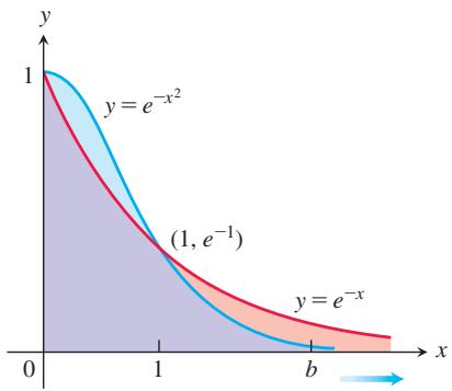
FIGURE 8.19 The graph of $𝑒 - 𝑥 2$ lies below the graph of $𝑒 - 𝑥$ for x > 1 (Example 6a).

HISTORICAL BIOGRAPHY Karl Weierstrass (1815–1897)

Weierstrass attended the University of Bonn to learn public administration, but he found that his passion was for mathematics. In his Berlin lectures in the 1860s, he also proved several theorems for continuous and complex functions. The standards of rigor that he set greatly affected the future of mathematics.

To obtain a numerical result with six digits, use the command “N[%, 6]”; it also yields 1.14579.

To know more, visit the companion Website.

Tests for Convergence and Divergence

When we cannot evaluate an improper integral directly, we try to determine whether it converges or diverges. If the integral diverges, that’s the end of the story. If it converges, we can use numerical methods to approximate its value. The principal tests for convergence or divergence are the Direct Comparison Test and the Limit Comparison Test.

THEOREM 2—Direct Comparison Test Let f and g be continuous on $[𝑎, \infty)$ with $0 \leq 𝑓 (𝑥) \leq 𝑔 (𝑥)$ for all $𝑥 \geq 𝑎$ . Then

if $\int \infty 𝑎 𝑔 (𝑥) 𝑑 𝑥$ converges, then $\int \infty 𝑎 𝑓 (𝑥) 𝑑 𝑥$ also converges.
if $\int \infty 𝑎 𝑓 (𝑥) 𝑑 𝑥$ diverges, then $\int \infty 𝑎 𝑔 (𝑥) 𝑑 𝑥$ also diverges.

Outline of a Proof Assume that $\int \infty 𝑎 𝑔 (𝑥) 𝑑 𝑥$ converges. For each number $𝑏 \geq 𝑎$ , let $𝐼 (𝑏) = \int 𝑏 𝑎 𝑓 (𝑥) 𝑑 𝑥$ . Since $𝑓 (𝑥)$ is nonnegative, we know that $𝐼 (𝑏)$ is an increasing function of b. Using the completeness property of the real numbers (Appendix A.7), it can be shown that since this integral increases with b, it either has a limit or it diverges to infinity as $𝑏 \to \infty$ . We will not give a proof of this fact here. Since $𝑓 (𝑥) \leq 𝑔 (𝑥)$ for every x,

𝐼 (𝑏) = \int 𝑏 𝑎 𝑓 (𝑥) 𝑑 𝑥 \leq \int 𝑏 𝑎 𝑔 (𝑥) 𝑑 𝑥 \leq \int \infty 𝑎 𝑔 (𝑥) 𝑑 𝑥 .

Thus, the finite number $𝑀 = \int \infty 𝑎 𝑔 (𝑥) 𝑑 𝑥$ is an upper bound to the values of $𝐼 (𝑏)$ . Therefore $𝐼 (𝑏)$ cannot diverge to infinity, so it must must converge to a finite value as $𝑏 \to \infty$ . Hence $\int \infty 𝑎 𝑓 (𝑥) 𝑑 𝑥$ converges. This establishes that statement 1 holds. Since statement 2 is the contrapositive form of statement 1, it must hold as well.

Although the theorem is stated for Type I improper integrals, a similar result is true for integrals of Type II as well.

EXAMPLE 6 These examples illustrate how we use Theorem 2.

(a) $\int \infty 1 𝑒 - 𝑥 2 𝑑 𝑥$ converges because $0 < 𝑒 - 𝑥 2 < 𝑒 - 𝑥$ for every $𝑥 \geq 1$ (Figure 8.19) and

\int \infty 1 𝑒 - 𝑥 𝑑 𝑥 = l i m 𝑏 \to \infty \int 𝑏 1 𝑒 - 𝑥 𝑑 𝑥 = l i m 𝑏 \to \infty [- 𝑒 - 𝑥 𝑑 𝑥] 𝑏 1 = l i m 𝑏 \to \infty (- 𝑒 - 𝑏 + 𝑒 - 1) = 1 𝑒

converges.

(b) $\int \infty 1 s i n 2 𝑥 𝑥 2 𝑑 𝑥$ converges because

0 \leq s i n 2 𝑥 𝑥 2 \leq 1 𝑥 2 o n [1, \infty) a n d \int \infty 1 1 𝑥 2 𝑑 𝑥 c o n v e r g e s . (E x a m p l e 3)

\int \infty 1 1 \sqrt 𝑥 2 - 0.1 𝑑 𝑥 d i v e r g e s b e c a u s e (c)

1 \sqrt 𝑥 2 - 0.1 \geq 1 𝑥 o n [1, \infty) a n d \int \infty 1 1 𝑥 𝑑 𝑥 d i v e r g e s . (E x a m p l e 3)

(d) $\int 𝜋 / 2 0 c o s 𝑥 \sqrt 𝑥 𝑑 𝑥$ converges because

0 \leq c o s 𝑥 \sqrt 𝑥 \leq 1 \sqrt 𝑥 o n [0, 𝜋 2], 0 \leq c o s 𝑥 \leq 1 o n [0, 𝜋 2]

and

\int 𝜋 / 2 0 𝑑 𝑥 \sqrt 𝑥 = l i m 𝑎 \to 0 + \int 𝜋 / 2 𝑎 𝑑 𝑥 \sqrt 𝑥 = l i m 𝑎 \to 0 + \sqrt 4 𝑥 ∣ 𝜋 / 2 𝑎 2 \sqrt 𝑥 = \sqrt 4 𝑥 = l i m 𝑎 \to 0 + (\sqrt 2 𝜋 - \sqrt 4 𝑎) = \sqrt 2 𝜋 c o n v e r g e s .

Although we have shown that the integrals in parts (a), (b), and (d) of Example 6 converge, we do not know the exact values of these integrals. For example, our computations in part (d) imply that

0 \leq \int 𝜋 / 2 0 c o s 𝑥 \sqrt 𝑥 𝑑 𝑥 \leq \int 𝜋 / 2 0 𝑑 𝑥 \sqrt 𝑥 = \sqrt 2 𝜋,

but unless we do further calculations the most we can say is that the integral is some real number between 0 and $\sqrt 2 𝜋$ .

THEOREM 3—Limit Comparison Test

If the positive functions $𝑓$ and $𝑔$ are continuous on $[𝑎, \infty)$ , and if

l i m 𝑥 \to \infty 𝑓 (𝑥) 𝑔 (𝑥) = 𝐿, 0 < 𝐿 < \infty,

then

\int \infty 𝑎 𝑓 (𝑥) 𝑑 𝑥 a n d \int \infty 𝑎 𝑔 (𝑥) 𝑑 𝑥

either both converge or both diverge.

We omit the proof of Theorem 3, which is similar to that of Theorem 2.

If two functions $𝑓 (𝑥)$ and $𝑔 (𝑥)$ satisfy the hypotheses of Theorem 3 and their improper integrals both converge, it need not be the case that these two integrals have the same value. This is illustrated in the next example.

EXAMPLE 7 Show that

\int \infty 1 𝑑 𝑥 1 + 𝑥 2

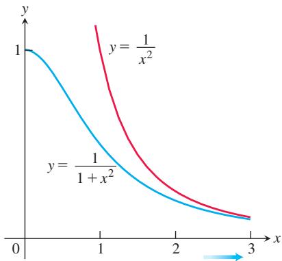
converges by comparison with $\int \infty 1 (1 / 𝑥 2) 𝑑 𝑥$ . Find and compare the values of the two integrals.

教材插图

Solution The functions $𝑓 (𝑥) = 1 / 𝑥 2$ and $𝑔 (𝑥) = 1 / (1 + 𝑥 2)$ are positive and continuous on $[1, \infty)$ . Also,

l i m 𝑥 \to \infty 𝑓 (𝑥) 𝑔 (𝑥) = l i m 𝑥 \to \infty 1 / 𝑥 2 1 / (1 + 𝑥 2) = l i m 𝑥 \to \infty 1 + 𝑥 2 𝑥 2 = l i m 𝑥 \to \infty (1 𝑥 2 + 1) = 0 + 1 = 1,

which is a positive finite limit (Figure 8.20). Therefore, $\int \infty 1 𝑑 𝑥 1 + 𝑥 2$ converges because $\int \infty 1 𝑑 𝑥 𝑥 2$ converges.

FIGURE 8.20 The functions in Example 7.

The integrals converge to different values, however:

\int \infty 1 𝑑 𝑥 𝑥 2 = 1 2 - 1 = 1 E x a m p l e 3

and

\int \infty 1 𝑑 𝑥 1 + 𝑥 2 = l i m 𝑏 \to \infty \int 𝑏 1 𝑑 𝑥 1 + 𝑥 2 = l i m 𝑏 \to \infty [t a n - 1 𝑏 - t a n - 1 1] = 𝜋 2 - 𝜋 4 = 𝜋 4 .

TABLE 8.5

b	$\int 𝑏 1 1 - 𝑒 - 𝑥 𝑥 𝑑 𝑥$
2	0.5226637569
5	1.3912002736
10	2.0832053156
100	4.3857862516
1000	6.6883713446
10000	8.9909564376
100000	11.2935415306

EXAMPLE 8 Investigate the convergence of $\int \infty 1 1 - 𝑒 - 𝑥 𝑥 𝑑 𝑥$ .

Solution The integrand suggests a comparison of $𝑓 (𝑥) = (1 - 𝑒 - 𝑥) / 𝑥$ with $𝑔 (𝑥) = 1 / 𝑥$ . However, we cannot use the Direct Comparison Test because $𝑓 (𝑥) \leq 𝑔 (𝑥)$ and the integral of $𝑔 (𝑥)$ diverges. On the other hand, using the Limit Comparison Test, we find that

l i m 𝑥 \to \infty 𝑓 (𝑥) 𝑔 (𝑥) = l i m 𝑥 \to \infty (1 - 𝑒 - 𝑥 𝑥) (𝑥 1) = l i m 𝑥 \to \infty (1 - 𝑒 - 𝑥) = 1,

which is a positive finite limit. Therefore, $\int \infty 1 1 - 𝑒 - 𝑥 𝑥 𝑑 𝑥$ diverges because $\int \infty 1 𝑑 𝑥 𝑥$ diverges. Approximations to the improper integral are given in Table 8.5. Note that the values of these approximations do not appear to approach a fixed finite limit as $𝑏 \to \infty$ .

EXERCISES 8.8

Evaluating Improper Integrals

The integrals in Exercises 1–34 converge. Evaluate the integrals without using tables.

$\int \infty 0 𝑑 𝑥 𝑥 2 + 1$
$\int \infty 1 𝑑 𝑥 𝑥 1.001$
$\int 10 𝑑 𝑥 \sqrt 𝑥$
$\int 40 𝑑 𝑥 \sqrt 4 - 𝑥$
$\int 1 - 1 𝑑 𝑥 𝑥 2 / 3$
$\int 1 - 8 𝑑 𝑥 𝑥 1 / 3$
$\int 10 𝑑 𝑥 \sqrt 1 - 𝑥 2$
$\int 10 𝑑 𝑟 𝑟 0.999$
$\int - 2 - \infty 2 𝑑 𝑥 𝑥 2 - 1$
$\int 2 - \infty 2 𝑑 𝑥 𝑥 2 + 4$
$\int \infty 2 2 𝑣 2 - 𝑣 𝑑 𝑣$
$\int \infty 2 2 𝑑 𝑡 𝑡 2 - 1$
$\int \infty - \infty 2 𝑥 𝑑 𝑥 (𝑥 2 + 1) 2$
$\int \infty - \infty 𝑥 𝑑 𝑥 (𝑥 2 + 4) 3 / 2$
$\int 10 𝜃 + 1 \sqrt 𝜃 2 + 2 𝜃 𝑑 𝜃$
$\int 20 𝑠 + 1 \sqrt 4 - 𝑠 2 𝑑 𝑠$
$\int \infty 0 𝑑 𝑥 (1 + 𝑥) \sqrt 𝑥$
$\int \infty 1 1 𝑥 \sqrt 𝑥 2 - 1 𝑑 𝑥$
$\int \infty 0 𝑑 𝑣 (1 + 𝑣 2) (1 + t a n - 1 𝑣)$
$\int \infty 0 16 t a n - 1 𝑥 1 + 𝑥 2 𝑑 𝑥$
$\int 0 - \infty 𝜃 𝑒 𝜃 𝑑 𝜃$
$\int \infty 0 2 𝑒 - 𝜃 s i n 𝜃 𝑑 𝜃$
$\int 0 - \infty 𝑒 - | 𝑥 | 𝑑 𝑥$
$\int \infty - \infty 2 𝑥 𝑒 - 𝑥 2 𝑑 𝑥$
$\int 10 𝑥 l n 𝑥 𝑑 𝑥$
$\int 10 (- l n 𝑥) 𝑑 𝑥$
$\int 20 𝑑 𝑠 \sqrt 4 - 𝑠 2$
$\int 10 4 𝑟 𝑑 𝑟 \sqrt 1 - 𝑟 4$
$\int 21 𝑑 𝑠 𝑠 \sqrt 𝑠 2 - 1$
$\int 42 𝑑 𝑡 𝑡 \sqrt 𝑡 2 - 4$
$\int 4 - 1 𝑑 𝑥 \sqrt | 𝑥 |$
$\int 20 𝑑 𝑥 \sqrt | 𝑥 - 1 |$
$\int \infty - 1 𝑑 𝜃 𝜃 2 + 5 𝜃 + 6$
$\int \infty 0 𝑑 𝑥 (𝑥 + 1) (𝑥 2 + 1)$

Testing for Convergence

In Exercises 35–68, use integration, the Direct Comparison Test, or the Limit Comparison Test to test the integrals for convergence. If more than one method applies, use whatever method you prefer.

$\int 2 1 / 2 𝑑 𝑥 𝑥 l n 𝑥$
$\int 1 - 1 𝑑 𝜃 𝜃 2 - 2 𝜃$
$\int \infty 1 / 2 𝑑 𝑥 𝑥 (l n 𝑥) 3$
$\int \infty 0 𝑑 𝜃 𝜃 2 - 1$
$\int 𝜋 / 2 0 t a n 𝜃 𝑑 𝜃$
$\int 𝜋 / 2 0 c o t 𝜃 𝑑 𝜃$
$\int 10 l n 𝑥 𝑥 2 𝑑 𝑥$
$\int 21 𝑑 𝑥 𝑥 l n 𝑥$

Theory and Examples

$\int l n 2 0 𝑥 - 2 𝑒 - 1 / 𝑥 𝑑 𝑥$
$\int 10 𝑒 - \sqrt 𝑥 \sqrt 𝑥 𝑑 𝑥$
$\int 𝜋 0 𝑑 𝑡 \sqrt 𝑡 + s i n 𝑡$
$\int 10 𝑑 𝑡 𝑡 - s i n 𝑡$ (Hint: $𝑡 \geq s i n 𝑡$ for $𝑡 \geq 0$ )
$\int 20 𝑑 𝑥 1 - 𝑥 2$
$\int 20 𝑑 𝑥 1 - 𝑥$
$\int 1 - 1 l n | 𝑥 | 𝑑 𝑥$

diverges and hence that

$\int 1 - 1 - 𝑥 l n | 𝑥 | 𝑑 𝑥$

\int \infty - \infty 2 𝑥 𝑑 𝑥 𝑥 2 + 1

$\int \infty 1 𝑑 𝑥 𝑥 3 + 1$
$\int \infty 4 𝑑 𝑥 \sqrt 𝑥 - 1$
$\int \infty 2 𝑑 𝑣 \sqrt 𝑣 - 1$
$\int \infty 0 𝑑 𝜃 1 + 𝑒 𝜃$
$\int \infty 0 𝑑 𝑥 \sqrt 𝑥 6 + 1$
$\int \infty 2 𝑑 𝑥 \sqrt 𝑥 2 - 1$

diverges. Then show that

$\int \infty 1 \sqrt 𝑥 + 1 𝑥 2 𝑑 𝑥$
$\int \infty 2 𝑥 𝑑 𝑥 \sqrt 𝑥 4 - 1$

$l i m 𝑏 \to \infty \int 𝑏 - 𝑏 2 𝑥 𝑑 𝑥 𝑥 2 + 1 = 0 .$

$\int \infty 𝜋 2 + c o s 𝑥 𝑥 𝑑 𝑥$
$\int \infty 𝜋 1 + s i n 𝑥 𝑥 2 𝑑 𝑥$

Exercises 83–86 are about the infinite region in the first quadrant between the curve $𝑦 = 𝑒 - 𝑥$ and the x-axis.

$\int \infty 4 2 𝑑 𝑡 𝑡 3 / 2 - 1$
$\int \infty 2 1 l n 𝑥 𝑑 𝑥$
$\int \infty 1 𝑒 𝑥 𝑥 𝑑 𝑥$
$\int \infty 𝑒 𝑒 l n (l n 𝑥) 𝑑 𝑥$
$\int \infty 1 1 \sqrt 𝑒 𝑥 - 𝑥 𝑑 𝑥$
$\int \infty 1 1 𝑒 𝑥 - 2 𝑥 𝑑 𝑥$
$\int \infty - \infty 𝑑 𝑥 \sqrt 𝑥 4 + 1$
$\int \infty - \infty 𝑑 𝑥 𝑒 𝑥 + 𝑒 - 𝑥$

In Exercises 69–80, determine whether the improper integral converges or diverges. If it converges, evaluate the integral.

$\int 10 1 𝑥 \sqrt 𝑥 𝑑 𝑥$
$\int \infty 2 1 𝑥 \sqrt 𝑥 𝑑 𝑥$
$\int 320 1 5 \sqrt 𝑥 𝑑 𝑥$
$\int \infty 1 1 5 \sqrt 𝑥 𝑑 𝑥$
$\int \infty 3 1 𝑥 4 𝑑 𝑥$
$\int 1 - 2 1 𝑥 4 𝑑 𝑥$
$\int \infty 0 𝑥 2 𝑒 𝑥 3 𝑑 𝑥$
$\int 0 - \infty 𝑥 2 𝑒 𝑥 3 𝑑 𝑥$
$\int 0 - 3 1 𝑥 2 + 3 𝑥 𝑑 𝑥$
$\int \infty 1 1 𝑥 2 + 3 𝑥 𝑑 𝑥$
$\int 4 - \infty 𝑥 (𝑥 2 + 9) 5 / 2 𝑑 𝑥$
$\int 4 - \infty 𝑥 (𝑥 2 + 9) 2 / 5 𝑑 𝑥$
Find the values of $𝑝$ for which each integral converges. a. $\int 21 𝑑 𝑥 𝑥 (l n 𝑥) 𝑝$ b. $\int \infty 2 𝑑 𝑥 𝑥 (l n 𝑥) 𝑝$
$\int \infty - \infty 𝑓 (𝑥) 𝑑 𝑥$ may not equal $l i m 𝑏 \to \infty \int 𝑏 - 𝑏 𝑓 (𝑥) 𝑑 𝑥 .$ Show that $\int \infty 0 2 𝑥 𝑑 𝑥 𝑥 2 + 1$
Find the area of the region.
Find the centroid of the region.
Find the volume of the solid generated by revolving the region about the y-axis.
Find the volume of the solid generated by revolving the region about the x-axis.
Find the area of the region that lies between the curves $𝑦 = s e c 𝑥$ and $𝑦 = t a n 𝑥$ from $𝑥 = 0$ to $𝑥 = 𝜋 / 2$ .
The region in Exercise 87 is revolved about the $𝑥$ -axis to generate a solid.

a. Find the volume of the solid.

b. Show that the inner and outer surfaces of the solid have infinite area.

Consider the infinite region in the first quadrant bounded by the graphs of $𝑦 = 1 𝑥 2$ , $𝑦 = 0$ , and $𝑥 = 1$ .

a. Find the area of the region.

b. Find the volume of the solid formed by revolving the region (i) about the x-axis; (ii) about the y-axis.

Consider the infinite region in the first quadrant bounded by the graphs of $𝑦 = 1 \sqrt 𝑥$ , $𝑦 = 0$ , $𝑥 = 0$ , and $𝑥 = 1$ .

a. Find the area of the region.

b. Find the volume of the solid formed by revolving the region (i) about the x-axis; (ii) about the y-axis.

Evaluate the integrals.

a. $\int 10 𝑑 𝑡 \sqrt 𝑡 (1 + 𝑡)$

𝐛 . \int \infty 0 𝑑 𝑡 \sqrt 𝑡 (1 + 𝑡)

Evaluate $\int \infty 3 𝑑 𝑥 𝑥 \sqrt 𝑥 2 - 9$
Estimating the value of a convergent improper integral whose domain is infinite

a. Show that

\int \infty 3 𝑒 - 3 𝑥 𝑑 𝑥 = 13 𝑒 - 9 < 0 . 000042,

and hence that $\int \infty 3 𝑒 - 𝑥 2 𝑑 𝑥 < 0.000042$ . Explain why this means that $\int \infty 0 𝑒 - 𝑥 2 𝑑 𝑥$ can be replaced by $\int 30 𝑒 - 𝑥 2 𝑑 𝑥$ without introducing an error of magnitude greater than 0.000042.

T b. Evaluate $\int 30 𝑒 - 𝑥 2 𝑑 𝑥$ numerically.

The infinite paint can or Gabriel’s horn As Example 3 shows, the integral $\int \infty 1 (𝑑 𝑥 / 𝑥)$ diverges. This means that the integral

\int \infty 1 2 𝜋 1 𝑥 \sqrt 1 + 1 𝑥 4 𝑑 𝑥,

which measures the surface area of the solid of revolution traced out by revolving the curve $𝑦 = 1 / 𝑥, 1 \leq 𝑥$ , about the x-axis, diverges also. By comparing the two integrals, we see that, for every finite value b > 1,

\int 𝑏 1 2 𝜋 1 𝑥 \sqrt 1 + 1 𝑥 4 𝑑 𝑥 > 2 𝜋 \int 𝑏 1 1 𝑥 𝑑 𝑥 .

教材插图

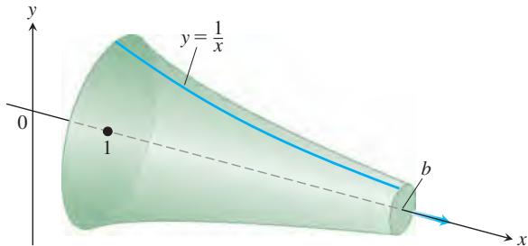
However, the integral

\int \infty 1 𝜋 (1 𝑥) 2 𝑑 𝑥

for the volume of the solid converges.

a. Calculate it.

b. This solid of revolution is sometimes described as a can that does not hold enough paint to cover its own interior. Think about that for a moment. It is common sense that a finite

amount of paint cannot cover an infinite surface. But if we fill the horn with paint (a finite amount), then we will have covered an infinite surface. Explain the apparent contradiction.

Sine-integral function The integral

S i (𝑥) = \int 𝑥 0 s i n 𝑡 𝑡 𝑑 𝑡,

called the sine-integral function, has important applications in optics.

T a. Plot the integrand $(s i n 𝑡) / 𝑡$ for t > 0. Is the sine-integral function everywhere increasing or decreasing? Do you think $S i (𝑥) = 0$ for $𝑥 \geq 0$ ? Check your answers by graphing the function $S i (𝑥)$ for $0 \leq 𝑥 \leq 25$ .

b. Explore the convergence of

\int \infty 0 s i n 𝑡 𝑡 𝑑 𝑡 .

If it converges, what is its value?

Error function The function

e r f (𝑥) = \int 𝑥 0 2 𝑒 - 𝑡 2 \sqrt 𝜋 𝑑 𝑡,

called the error function, has important applications in probability and statistics.

T a. Plot the error function for $0 \leq 𝑥 \leq 25$ .

b. Explore the convergence of

\int \infty 0 2 𝑒 - 𝑡 2 \sqrt 𝜋 𝑑 𝑡 .

If it converges, what appears to be its value? You will see how to confirm your estimate in Section 14.4, Exercise 41.

Normal probability distribution The function

𝑓 (𝑥) = 1 𝜎 \sqrt 2 𝜋 𝑒 - 12 (𝑥 - 𝜇 𝜎) 2

is called the normal probability density function with mean $𝜇$ and standard deviation $𝜎$ . The number $𝜇$ tells where the distribution is centered, and $𝜎$ measures the “scatter” around the mean.

From the theory of probability, it is known that

\int \infty - \infty 𝑓 (𝑥) 𝑑 𝑥 = 1 .

In what follows, let $𝜇 = 0$ and $𝜎 = 1$ .

T a. Draw the graph of f. Find the intervals on which f is increasing, the intervals on which f is decreasing, and any local extreme values and where they occur.

b. Evaluate

\int 𝑛 - 𝑛 𝑓 (𝑥) 𝑑 𝑥

for n = 1, 2, and 3.

c. Give a convincing argument that

\int \infty - \infty 𝑓 (𝑥) 𝑑 𝑥 = 1 .

(Hint: Show that $0 < 𝑓 (𝑥) < 𝑒 - 𝑥 / 2$ for $𝑥 > 1$ , and for $𝑏 > 1$ ,

\int \infty 𝑏 𝑒 - 𝑥 / 2 𝑑 𝑥 \to 0 a s 𝑏 \to \infty .)

Show that if $𝑓 (𝑥)$ is integrable on every interval of real numbers, and if a and b are real numbers with a < b, then

a. $\int 𝑎 - \infty 𝑓 (𝑥) 𝑑 𝑥$ and $\int \infty 𝑎 𝑓 (𝑥) 𝑑 𝑥$ both converge if and only if

$\int 𝑏 - \infty 𝑓 (𝑥) 𝑑 𝑥$ and $\int \infty 𝑏 𝑓 (𝑥) 𝑑 𝑥$ both converge.

𝐛 . \int 𝑎 - \infty 𝑓 (𝑥) 𝑑 𝑥 + \int \infty 𝑎 𝑓 (𝑥) 𝑑 𝑥 = \int 𝑏 - \infty 𝑓 (𝑥) 𝑑 𝑥 + \int \infty 𝑏 𝑓 (𝑥) 𝑑 𝑥

when the integrals involved converge.

COMPUTER EXPLORATIONS

In Exercises 99–102, use a CAS to explore the integrals for various values of p (include noninteger values). For what values of p does the

$\int \infty 𝑒 𝑥 𝑝 l n 𝑥 𝑑 𝑥$

integral converge? What is the value of the integral when it does converge? Plot the integrand for various values of p.

$\int \infty 0 𝑥 𝑝 l n 𝑥 𝑑 𝑥$
$\int \infty - \infty 𝑥 𝑝 l n | 𝑥 | 𝑑 𝑥$

Use a CAS to evaluate the integrals.

$\int 2 / 𝜋 0 s i n 1 𝑥 𝑑 𝑥$
$\int 2 / 𝜋 0 𝑥 s i n 1 𝑥 𝑑 𝑥$

CHAPTER 8 Questions to Guide Your Review

What is the formula for integration by parts? Where does it come from? Why might you want to use it?
When applying the formula for integration by parts, how do you choose the u and dv? How can you apply integration by parts to an integral of the form $\int 𝑓 (𝑥) 𝑑 𝑥$ ?
If an integrand is a product of the form $s i n 𝑛 𝑥 c o s 𝑚 𝑥$ , where m and n are nonnegative integers, how do you evaluate the integral? Give a specific example of each case.
What substitutions are made to evaluate integrals of $s i n 𝑚 𝑥$ sin nx, $s i n 𝑚 𝑥 c o s 𝑛 𝑥$ , and $c o s 𝑚 𝑥 c o s 𝑛 𝑥$ ? Give an example of each case.
$\int 𝑒 0 𝑥 𝑝 l n 𝑥 𝑑 𝑥$
What substitutions are sometimes used to transform integrals involving $\sqrt 𝑎 2 - 𝑥 2$ , $\sqrt 𝑎 2 + 𝑥 2$ , and $\sqrt 𝑥 2 - 𝑎 2$ into integrals that can be evaluated directly? Give an example of each case.
What restrictions can you place on the variables involved in the three basic trigonometric substitutions to make sure the substitutions are reversible (have inverses)?
What is the goal of the method of partial fractions?
When the degree of a polynomial $𝑓 (𝑥)$ is less than the degree of a polynomial $𝑔 (𝑥)$ , how do you write $𝑓 (𝑥) / 𝑔 (𝑥)$ as a sum of partial fractions if $𝑔 (𝑥)$

a. is a product of distinct linear factors?

b. consists of a repeated linear factor?

c. contains an irreducible quadratic factor?

What do you do if the degree of $𝑓$ is not less than the degree of $𝑔$ ?

How are integral tables typically used? What do you do if a particular integral you want to evaluate is not listed in the table?
What is a reduction formula? How are reduction formulas used? Give an example.
How would you compare the relative merits of the Midpoint Rule, the Trapezoidal Rule, and Simpson’s Rule?
What is an improper integral of Type I? Type II? How are the values of various types of improper integrals defined? Give examples.
What tests are available for determining the convergence and divergence of improper integrals that cannot be evaluated directly? Give examples of their use.
What is a random variable? What is a continuous random variable? Give some specific examples.
What is a probability density function? What is the probability that a continuous random variable has a value in the interval $[𝑐, 𝑑]$ ?
What is an exponentially decreasing probability density function? What are some typical events that might be modeled by this distribution? What do we mean when we say such distributions are memoryless?
What is the expected value of a continuous random variable? What is the expected value of an exponentially distributed random variable?
What is the median of a continuous random variable? What is the median of an exponential distribution?
What does the variance of a random variable measure? What is the standard deviation of a continuous random variable $𝑋$ ?
What probability density function describes the normal distribution? What are some examples typically modeled by a normal distribution? How do we usually calculate probabilities for a normal distribution?
In a normal distribution, what percentage of the population lies within 1 standard deviation of the mean? Within 2 standard deviations?

CHAPTER 8 Practice Exercises

Integration by Parts

Evaluate the integrals in Exercises 1–8 using integration by parts.

$\int l n (𝑥 + 1) 𝑑 𝑥$
$\int 𝑥 2 l n 𝑥 𝑑 𝑥$
$\int a r c t a n 3 𝑥 𝑑 𝑥$
$\int c o s - 1 (𝑥 2) 𝑑 𝑥$
$\int (𝑥 + 1) 2 𝑒 𝑥 𝑑 𝑥$
$\int 𝑥 2 s i n (1 - 𝑥) 𝑑 𝑥$
$\int 𝑒 𝑥 c o s 2 𝑥 𝑑 𝑥$
$\int 𝑥 s i n 𝑥 c o s 𝑥 𝑑 𝑥$

Partial Fractions

Evaluate the integrals in Exercises 9–28. It may be necessary to use a substitution first.

$\int 𝑥 𝑑 𝑥 𝑥 2 - 3 𝑥 + 2$
$\int 𝑥 𝑑 𝑥 𝑥 2 + 4 𝑥 + 3$
$\int 𝑑 𝑥 𝑥 (𝑥 + 1) 2$
$\int 𝑥 + 1 𝑥 2 (𝑥 - 1) 𝑑 𝑥$
$\int s i n 𝜃 𝑑 𝜃 c o s 2 𝜃 + c o s 𝜃 - 2$
$\int c o s 𝜃 𝑑 𝜃 s i n 2 𝜃 + s i n 𝜃 - 6$
$\int 3 𝑥 2 + 4 𝑥 + 4 𝑥 3 + 𝑥 𝑑 𝑥$
$\int 4 𝑥 𝑑 𝑥 𝑥 3 + 4 𝑥$
$\int 𝑣 + 3 2 𝑣 3 - 8 𝑣 𝑑 𝑣$
$\int (3 𝑣 - 7) 𝑑 𝑣 (𝑣 - 1) (𝑣 - 2) (𝑣 - 3)$
$\int 𝑑 𝑡 𝑡 4 + 4 𝑡 2 + 3$
$\int 𝑡 𝑑 𝑡 𝑡 4 - 𝑡 2 - 2$
$\int 𝑥 3 + 𝑥 2 𝑥 2 + 𝑥 - 2 𝑑 𝑥$
$\int 𝑥 3 + 1 𝑥 3 - 𝑥 𝑑 𝑥$
$\int 𝑥 3 + 4 𝑥 2 𝑥 2 + 4 𝑥 + 3 𝑑 𝑥$
$\int 2 𝑥 3 + 𝑥 2 - 21 𝑥 + 24 𝑥 2 + 2 𝑥 - 8 𝑑 𝑥$
$\int 𝑑 𝑥 𝑥 (3 \sqrt 𝑥 + 1)$
$\int 𝑑 𝑥 𝑥 (1 + 3 \sqrt 𝑥)$
$\int 𝑑 𝑠 𝑒 𝑠 - 1$
$\int 𝑑 𝑠 \sqrt 𝑒 𝑠 + 1$

Trigonometric Substitutions

Evaluate the integrals in Exercises 29–32 (a) without using a trigonometric substitution, (b) using a trigonometric substitution.

$\int 𝑦 𝑑 𝑦 \sqrt 16 - 𝑦 2$
$\int 𝑥 𝑑 𝑥 \sqrt 4 + 𝑥 2$
$\int 𝑥 𝑑 𝑥 4 - 𝑥 2$

\int 𝑡 𝑑 𝑡 \sqrt 4 𝑡 2 - 1

Evaluate the integrals in Exercises 33–36. 33. $\int 𝑥 𝑑 𝑥 9 - 𝑥 2$

$\int 𝑑 𝑥 𝑥 (9 - 𝑥 2)$
$\int 𝑑 𝑥 9 - 𝑥 2$
$\int 𝑑 𝑥 \sqrt 9 - 𝑥 2$

Trigonometric Integrals

Evaluate the integrals in Exercises 37–44.

$\int s i n 3 𝑥 c o s 4 𝑥 𝑑 𝑥$
$\int c o s 5 𝑥 s i n 5 𝑥 𝑑 𝑥$
$\int t a n 4 𝑥 s e c 2 𝑥 𝑑 𝑥$
$\int t a n 3 𝑥 s e c 3 𝑥 𝑑 𝑥$
$\int s i n 5 𝜃 c o s 6 𝜃 𝑑 𝜃$
$\int s e c 2 𝜃 s i n 3 𝜃 𝑑 𝜃$
$\int \sqrt 1 + c o s (𝑡 / 2) 𝑑 𝑡$
$\int 𝑒 𝑡 \sqrt t a n 2 𝑒 𝑡 + 1 𝑑 𝑡$

Numerical Integration

According to the error-bound formula for Simpson’s Rule, how many subintervals should you use to be sure of estimating the value of

l n 3 = \int 31 1 𝑥 𝑑 𝑥

by Simpson’s Rule with an error of no more than $10 - 4$ in absolute value? (Remember that for Simpson’s Rule, the number of subintervals has to be even.)

A brief calculation shows that if $0 \leq 𝑥 \leq 1$ , then the second derivative of $𝑓 (𝑥) = \sqrt 1 + 𝑥 4$ lies between 0 and 8. Based on this, about how many subdivisions would you need to estimate the integral of $𝑓$ from 0 to 1 with an error no greater than $10 - 3$ in absolute value using the Trapezoidal Rule?
A direct calculation shows that

\int 𝜋 0 2 s i n 2 𝑥 𝑑 𝑥 = 𝜋 .

How close do you come to this value by using the Trapezoidal Rule with $𝑛 = 6$ ? The Midpoint Rule with $𝑛 = 6$ ? Simpson’s Rule with $𝑛 = 6$ ? Try them and find out.

You are planning to use Simpson’s Rule to estimate the value of the integral

\int 21 𝑓 (𝑥) 𝑑 𝑥

with an error magnitude less than $10 - 5$ . You have determined that $| 𝑓 (4) (𝑥) | \leq 3$ throughout the interval of integration. How many subintervals should you use to ensure the required accuracy? (Remember that for Simpson’s Rule, the number has to be even.)

T 49. Mean temperature Compute the average value of the temperature function

𝑓 (𝑥) = 20 s i n (2 𝜋 365 (𝑥 - 101)) - 4

for a 365-day year. This is one way to estimate the annual mean air temperature in Fairbanks, Alaska. The National Weather Service’s official figure, a numerical average of the daily normal mean air temperatures for the year, is $- 3.5 \circ C$ , which is slightly higher than the average value of $𝑓 (𝑥)$ .

Heat capacity of a gas Heat capacity $𝐶 𝑣$ is the amount of heat required to raise the temperature of a given mass of gas with constant volume by 1 °C, measured in units of cal/deg-mol (calories per degree gram molecular weight). The heat capacity of oxygen depends on its temperature T and satisfies the formula

𝐶 𝑣 = 8 . 27 + 1 0 - 5 (26 𝑇 - 1 . 87 𝑇 2) .

Use Simpson’s Rule to find the average value of $𝐶 𝑣$ and the temperature at which it is attained for $20 \circ C \leq 𝑇 \leq 675 \circ C$ .

Fuel efficiency An automobile computer gives a digital readout of fuel consumption in liters per hour. During a trip, a passenger recorded the fuel consumption every 5 min for a full hour of travel.

Time	L/h	Time	L/h
0	2.5	35	2.5
5	2.4	40	2.4
10	2.3	45	2.3
15	2.4	50	2.4
20	2.4	55	2.4
25	2.5	60	2.3
30	2.6

a. Use the Trapezoidal Rule to approximate the total fuel consumption during the hour.

b. If the automobile covered 60 km in the hour, what was its fuel efficiency (in kilometers per liter) for that portion of the trip?

A new parking lot To meet the demand for parking, your town has allocated the area shown here. As the town engineer, you have been asked by the town council to find out if the lot can be built for $11, 000 . 𝑇 ℎ 𝑒 𝑐 𝑜 𝑠 𝑡 𝑡 𝑜 𝑐 𝑙 𝑒 𝑎 𝑟 𝑡 ℎ 𝑒 𝑙 𝑎 𝑛 𝑑 𝑤 𝑖 𝑙 𝑙 𝑏 𝑒$ 1.00 a square meter, and the lot will cost $20.00 𝑎 𝑠 𝑞 𝑢 𝑎 𝑟 𝑒 𝑚 𝑒 𝑡 𝑒 𝑟 𝑡 𝑜 𝑝 𝑎 𝑣 𝑒 . 𝑈 𝑠 𝑒 𝑆 𝑖 𝑚 𝑝 𝑠 𝑜 𝑛' 𝑠 𝑅 𝑢 𝑙 𝑒 𝑡 𝑜 𝑓 𝑖 𝑛 𝑑 𝑜 𝑢 𝑡 𝑖 𝑓 𝑡 ℎ 𝑒 𝑗 𝑜 𝑏 𝑐 𝑎 𝑛 𝑏 𝑒 𝑑 𝑜 𝑛 𝑒 𝑓 𝑜 𝑟$ 11,000.

教材插图

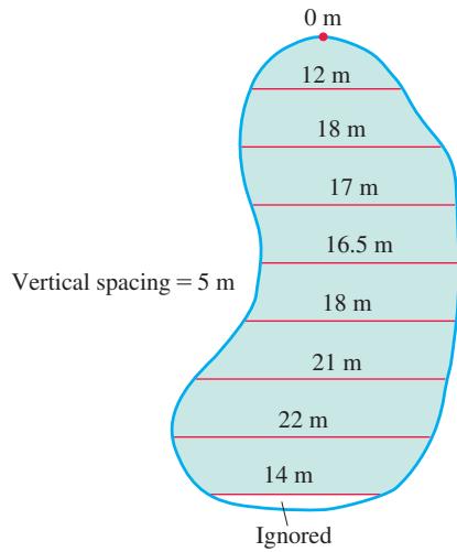
Improper Integrals

Evaluate the improper integrals in Exercises 53–62.

$\int 30 𝑑 𝑥 \sqrt 9 - 𝑥 2$
$\int 10 l n 𝑥 𝑑 𝑥$
$\int 20 𝑑 𝑦 (𝑦 - 1) 2 / 3$
$\int 0 - 2 𝑑 𝜃 (𝜃 + 1) 3 / 5$
$\int \infty 3 2 𝑑 𝑢 𝑢 2 - 2 𝑢$
$\int \infty 1 3 𝑣 - 1 4 𝑣 3 - 𝑣 2 𝑑 𝑣$
$\int \infty 0 𝑥 2 𝑒 - 𝑥 𝑑 𝑥$
$\int 0 - \infty 𝑥 𝑒 3 𝑥 𝑑 𝑥$
$\int \infty - \infty 𝑑 𝑥 4 𝑥 2 + 9$
$\int \infty - \infty 4 𝑑 𝑥 𝑥 2 + 16$

Which of the improper integrals in Exercises 63–68 converge and which diverge?

$\int \infty 6 𝑑 𝜃 \sqrt 𝜃 2 + 1$
$\int \infty 0 𝑒 - 𝑢 c o s 𝑢 𝑑 𝑢$
$\int \infty 1 l n 𝑧 𝑧 𝑑 𝑧$
$\int \infty 1 𝑒 - 𝑡 \sqrt 𝑡 𝑑 𝑡$
$\int \infty - \infty 2 𝑑 𝑥 𝑒 𝑥 + 𝑒 - 𝑥$
$\int \infty - \infty 𝑑 𝑥 𝑥 2 (1 + 𝑒 𝑥)$

Assorted Integrations

Evaluate the integrals in Exercises 69–134. The integrals are listed in random order so you need to decide which integration technique to use.

$\int 𝑥 𝑒 2 𝑥 𝑑 𝑥$
$\int 10 𝑥 2 𝑒 𝑥 3 𝑑 𝑥$
$\int (t a n 2 𝑥 + s e c 2 𝑥) 𝑑 𝑥$
$\int 𝜋 / 4 0 c o s 2 2 𝑥 𝑑 𝑥$
$\int 𝑥 s e c 2 𝑥 𝑑 𝑥$
$\int 𝑥 s e c 2 (𝑥 2) 𝑑 𝑥$
$\int s i n 𝑥 c o s 2 𝑥 𝑑 𝑥$
$\int s i n 2 𝑥 s i n (c o s 2 𝑥) 𝑑 𝑥$
$\int 0 - 1 𝑒 𝑥 𝑒 𝑥 + 𝑒 - 𝑥 𝑑 𝑥$
$\int (𝑒 2 𝑥 + 𝑒 - 𝑥) 2 𝑑 𝑥$
$\int 𝑥 + 1 𝑥 4 - 𝑥 3 𝑑 𝑥$
$\int 𝑒 𝑥 + 1 𝑒 𝑥 (𝑒 2 𝑥 - 4) 𝑑 𝑥$
$\int 𝑒 𝑥 + 𝑒 3 𝑥 𝑒 2 𝑥 𝑑 𝑥$
$\int (𝑒 𝑥 - 𝑒 - 𝑥) (𝑒 𝑥 + 𝑒 - 𝑥) 3 𝑑 𝑥$
$\int 𝜋 / 3 0 t a n 3 𝑥 s e c 2 𝑥 𝑑 𝑥$
$\int t a n 4 𝑥 s e c 4 𝑥 𝑑 𝑥$
$\int 30 (𝑥 + 2) \sqrt 𝑥 + 1 𝑑 𝑥$
$\int (𝑥 + 1) \sqrt 𝑥 2 + 2 𝑥 𝑑 𝑥$
$\int c o t 𝑥 c s c 3 𝑥 𝑑 𝑥$
$\int s i n 𝑥 (t a n 𝑥 - c o t 𝑥) 2 𝑑 𝑥$
$\int 𝑥 𝑑 𝑥 1 + \sqrt 𝑥$
$\int 𝑥 3 + 2 4 - 𝑥 2 𝑑 𝑥$
$\int \sqrt 2 𝑥 - 𝑥 2 𝑑 𝑥$
$\int 𝑑 𝑥 \sqrt - 2 𝑥 - 𝑥 2$
$\int 2 - c o s 𝑥 + s i n 𝑥 s i n 2 𝑥 𝑑 𝑥$
$\int s i n 2 𝜃 c o s 5 𝜃 𝑑 𝜃$
$\int 9 𝑑 𝑣 81 - 𝑣 4$
$\int \infty 2 𝑑 𝑥 (𝑥 - 1) 2$
$\int 𝜃 c o s (2 𝜃 + 1) 𝑑 𝜃$
$\int 𝑥 3 𝑑 𝑥 𝑥 2 - 2 𝑥 + 1$
$\int s i n 2 𝜃 𝑑 𝜃 (1 + c o s 2 𝜃) 2$
$\int 𝜋 / 2 𝜋 / 4 \sqrt 1 + c o s 4 𝑥 𝑑 𝑥$
$\int 𝑥 𝑑 𝑥 \sqrt 2 - 𝑥$
$\int \sqrt 1 - 𝑣 2 𝑣 2 𝑑 𝑣$
$\int 𝑑 𝑦 𝑦 2 - 2 𝑦 + 2$
$\int 𝑥 𝑑 𝑥 \sqrt 8 - 2 𝑥 2 - 𝑥 4$
$\int 𝑧 + 1 𝑧 2 (𝑧 2 + 4) 𝑑 𝑧$
$\int 𝑥 2 (𝑥 - 1) 1 / 3 𝑑 𝑥$
$\int 𝑡 𝑑 𝑡 \sqrt 9 - 4 𝑡 2$
$\int a r c t a n 𝑥 𝑥 2 𝑑 𝑥$
$\int 𝑒 𝑡 𝑑 𝑡 𝑒 2 𝑡 + 3 𝑒 𝑡 + 2$
$\int t a n 3 𝑡 𝑑 𝑡$
$\int \infty 1 l n 𝑦 𝑦 3 𝑑 𝑦$
$\int 𝑦 3 / 2 (l n 𝑦) 2 𝑑 𝑦$
$\int 𝑒 l n \sqrt 𝑥 𝑑 𝑥$
$\int 𝑒 𝜃 \sqrt 3 + 4 𝑒 𝜃 𝑑 𝜃$
$\int s i n 5 𝑡 𝑑 𝑡 1 + (c o s 5 𝑡) 2$
$\int 𝑑 𝑣 \sqrt 𝑒 2 𝑣 - 1$
$\int 𝑑 𝑟 1 + \sqrt 𝑟$
$\int 4 𝑥 3 - 20 𝑥 𝑥 4 - 10 𝑥 2 + 9 𝑑 𝑥$
$\int 𝑥 3 1 + 𝑥 2 𝑑 𝑥$
$\int 𝑥 2 1 + 𝑥 3 𝑑 𝑥$
$\int 1 + 𝑥 2 1 + 𝑥 3 𝑑 𝑥$
$\int 1 + 𝑥 2 (1 + 𝑥) 3 𝑑 𝑥$
$\int \sqrt 𝑥 \cdot \sqrt 1 + \sqrt 𝑥 𝑑 𝑥$
$\int \sqrt 1 + \sqrt 1 + 𝑥 𝑑 𝑥$
$\int 1 \sqrt 𝑥 \cdot \sqrt 1 + 𝑥 𝑑 𝑥$
$\int 1 / 2 0 \sqrt 1 + \sqrt 1 - 𝑥 2 𝑑 𝑥$
$\int l n 𝑥 𝑥 + 𝑥 l n 𝑥 𝑑 𝑥$
$\int 1 𝑥 \cdot l n 𝑥 \cdot l n (l n 𝑥) 𝑑 𝑥$
$\int 𝑥 l n 𝑥 l n 𝑥 𝑥 𝑑 𝑥$
$\int (l n 𝑥) l n 𝑥 [1 𝑥 + l n (l n 𝑥) 𝑥] 𝑑 𝑥$
$\int 1 𝑥 \sqrt 1 - 𝑥 4 𝑑 𝑥$
$\int \sqrt 1 - 𝑥 𝑥 𝑑 𝑥$
$\int s i n 2 𝑥 1 + s i n 2 𝑥 𝑑 𝑥$
$\int 1 - c o s 𝑥 1 + c o s 𝑥 𝑑 𝑥$
Evaluate $\int 𝜋 / 2 0 s i n 𝑥 s i n 𝑥 + c o s 𝑥 𝑑 𝑥$ in two ways:

a. By evaluating $\int s i n 𝑥 s i n 𝑥 + c o s 𝑥 𝑑 𝑥$ , then using the Evaluation Theorem.

b. By showing that $\int 𝑎 0 𝑓 (𝑥) 𝑑 𝑥 = \int 𝑎 0 𝑓 (𝑎 - 𝑥) 𝑑 𝑥$ , then using this result.

CHAPTER 8 Additional and Advanced Exercises

Evaluating Integrals

Evaluate the integrals in Exercises 1–6.

$\int (a r c s i n 𝑥) 2 𝑑 𝑥$
$\int 𝑑 𝑥 𝑥 (𝑥 + 1) (𝑥 + 2) \dots (𝑥 + 𝑚)$
$\int 𝑥 a r c s i n 𝑥 𝑑 𝑥$
$\int s i n - 1 \sqrt 𝑦 𝑑 𝑦$
$\int 𝑑 𝑡 𝑡 - \sqrt 1 - 𝑡 2$
$\int 𝑑 𝑥 𝑥 4 + 4$

Evaluate the limits in Exercise 7 and 8.
7. $l i m 𝑥 \to \infty \int 𝑥 - 𝑥 s i n 𝑡 𝑑 𝑡$

$l i m 𝑥 \to 0 + 𝑥 \int 1 𝑥 c o s 𝑡 𝑡 2 𝑑 𝑡$

Evaluate the limits in Exercise 9 and 10 by identifying them with definite integrals and evaluating the integrals.

$l i m 𝑛 \to \infty \sum 𝑛 𝑘 = 1 l n 𝑛 \sqrt 1 + 𝑘 𝑛$
$l i m 𝑛 \to \infty \sum 𝑛 - 1 𝑘 = 0 1 \sqrt 𝑛 2 - 𝑘 2$

Applications

Finding arc length Find the length of the curve

𝑦 = \int 𝑥 0 \sqrt c o s 2 𝑡 𝑑 𝑡, 0 \leq 𝑥 \leq 𝜋 / 4 .

Finding arc length Find the length of the graph of the function $𝑦 = l n (1 - 𝑥 2)$ , $0 \leq 𝑥 \leq 1 / 2$ .
Finding volume The region in the first quadrant that is enclosed by the x-axis and the curve $𝑦 = 3 𝑥 \sqrt 1 - 𝑥$ is revolved about the y-axis to generate a solid. Find the volume of the solid.
Finding volume The region in the first quadrant that is enclosed by the x-axis, the curve $𝑦 = 5 / (𝑥 \sqrt 5 - 𝑥)$ , and the lines x = 1 and x = 4 is revolved about the x-axis to generate a solid. Find the volume of the solid.
Finding volume The region in the first quadrant enclosed by the coordinate axes, the curve $𝑦 = 𝑒 𝑥$ , and the line x = 1 is revolved about the y-axis to generate a solid. Find the volume of the solid.
Finding volume The region in the first quadrant that is bounded above by the curve $𝑦 = 𝑒 𝑥 - 1$ , below by the x-axis, and on the right by the line $𝑥 = l n 2$ is revolved about the line $𝑥 = l n 2$ to generate a solid. Find the volume of the solid.
Finding volume Let $𝑅$ be the “triangular” region in the first quadrant that is bounded above by the line $𝑦 = 1$ , below by the curve $𝑦 = l n 𝑥$ , and on the left by the line $𝑥 = 1$ . Find the volume of the solid generated by revolving $𝑅$ about a. the $𝑥$ -axis. b. the line $𝑦 = 1$ .
Finding volume (Continuation of Exercise 17.) Find the volume of the solid generated by revolving the region R about a. the y-axis. b. the line x = 1.
Finding volume The region between the x-axis and the curve

𝑦 = 𝑓 (𝑥) = {0, 𝑥 = 0 𝑥 l n 𝑥, 0 < 𝑥 \leq 2

is revolved about the x-axis to generate the solid shown here.

a. Show that $𝑓$ is continuous at $𝑥 = 0$ .

b. Find the volume of the solid.

教材插图

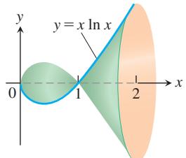
Finding volume The infinite region bounded by the coordinate axes and the curve $𝑦 = - l n 𝑥$ in the first quadrant is revolved about the x-axis to generate a solid. Find the volume of the solid.
Centroid of a region Find the centroid of the region in the first quadrant that is bounded below by the x-axis, above by the curve $𝑦 = l n 𝑥$ , and on the right by the line x = e.
Centroid of a region Find the centroid of the region in the plane enclosed by the curves $𝑦 = \pm (1 - 𝑥 2) - 1 / 2$ and the lines x = 0 and x = 1.
Length of a curve Find the length of the curve $𝑦 = l n 𝑥$ from $𝑥 = 1$ to $𝑥 = 𝑒$ .
Finding surface area Find the area of the surface generated by revolving the curve in Exercise 23 about the y-axis.
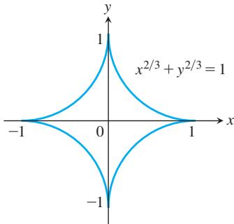
The surface generated by an astroid The graph of the equation $𝑥 2 / 3 + 𝑦 2 / 3 = 1$ is an astroid (see accompanying figure). Find the area of the surface generated by revolving the curve about the $𝑥$ -axis.

教材插图

Length of a curve Find the length of the curve

𝑦 = \int 𝑥 1 \sqrt \sqrt 𝑡 - 1 𝑑 𝑡, 1 \leq 𝑥 \leq 1 6 .

For what value or values of a does

\int \infty 1 (𝑎 𝑥 𝑥 2 + 1 - 1 2 𝑥) 𝑑 𝑥

converge? Evaluate the corresponding integral(s).

For each $𝑥 > 0$ , let $𝐺 (𝑥) = \int \infty 0 𝑒 - 𝑥 𝑡 𝑑 𝑡$ . Prove that $𝑥 𝐺 (𝑥) = 1$ for each $𝑥 > 0$ .
Infinite area and finite volume What values of $𝑝$ have the following property? The area of the region between the curve $𝑦 = 𝑥 - 𝑝$ , $1 \leq 𝑥 < \infty$ , and the $𝑥$ -axis is infinite but the volume of the solid generated by revolving the region about the $𝑥$ -axis is finite.
Infinite area and finite volume What values of p have the following property? The area of the region in the first quadrant enclosed by the curve $𝑦 = 𝑥 - 𝑝$ , the y-axis, the line x = 1, and the interval [0, 1] on the x-axis is infinite, but the volume of the solid generated by revolving the region about one of the coordinate axes is finite.
Integrating the square of the derivative If $𝑓$ is continuously differentiable on $[0, 1]$ , and $𝑓 (1) = 𝑓 (0) = - 1 / 6$ , prove that

\int 10 (𝑓' (𝑥)) 2 𝑑 𝑥 \geq 2 \int 10 𝑓 (𝑥) 𝑑 𝑥 + 14 .

Hint: Consider the inequality $0 \leq \int 10 (𝑓' (𝑥) + 𝑥 - 12) 2 𝑑 𝑥$ .

Source: Mathematics Magazine, vol. 84, no. 4, Oct. 2011.

(Continuation of Exercise 31.) If $𝑓$ is continuously differentiable on $[0, 𝑎]$ for $𝑎 > 0$ , and $𝑓 (𝑎) = 𝑓 (0) = 𝑏$ , prove that

\int 𝑎 0 (𝑓' (𝑥)) 2 𝑑 𝑥 \geq 2 \int 𝑎 0 𝑓 (𝑥) 𝑑 𝑥 - (2 𝑎 𝑏 + 𝑎 3 12) .

Hint: Consider the inequality $0 \leq \int 𝑎 0 (𝑓' (𝑥) + 𝑥 - 𝑎 2) 2 𝑑 𝑥$ . Source: Mathematics Magazine, vol. 84, no. 4, Oct. 2011.

The Substitution $𝑧 = t a n (𝑥 / 2)$ The substitution

𝑧 = t a n 𝑥 2 (1)

reduces the problem of integrating a rational expression in $s i n 𝑥$ and $c o s 𝑥$ to a problem of integrating a rational function of z. This in turn can be integrated by partial fractions.

From the accompanying figure

教材插图

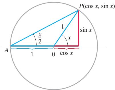
we can read the relation

t a n 𝑥 2 = s i n 𝑥 1 + c o s 𝑥 .

To see the effect of the substitution, we calculate

c o s 𝑥 = 2 c o s 2 (𝑥 2) - 1 = 2 s e c 2 (𝑥 / 2) - 1 = 2 1 + t a n 2 (𝑥 / 2) - 1 = 2 1 + 𝑧 2 - 1 c o s 𝑥 = 1 - 𝑧 2 1 + 𝑧 2, (2)

and

s i n 𝑥 = 2 s i n 𝑥 2 c o s 𝑥 2 = 2 s i n (𝑥 / 2) c o s (𝑥 / 2) \cdot c o s 2 (𝑥 2) = 2 t a n 𝑥 2 \cdot 1 s e c 2 (𝑥 / 2) = 2 t a n (𝑥 / 2) 1 + t a n 2 (𝑥 / 2) s i n 𝑥 = 2 𝑧 1 + 𝑧 2 . (3)

Finally, $𝑥 = 2 a r c t a n 𝑧$ , so

𝑑 𝑥 = 2 𝑑 𝑧 1 + 𝑧 2 . (4)

Examples

\int 1 1 + c o s 𝑥 𝑑 𝑥 = \int 1 + 𝑧 2 2 2 𝑑 𝑧 1 + 𝑧 2 = \int 𝑑 𝑧 = 𝑧 + 𝐶 = t a n (𝑥 2) + 𝐶

b . \int 1 2 + s i n 𝑥 𝑑 𝑥 = \int 1 + 𝑧 2 2 + 2 𝑧 + 2 𝑧 2 2 𝑑 𝑧 1 + 𝑧 2 = \int 𝑑 𝑧 𝑧 2 + 𝑧 + 1 = \int 𝑑 𝑧 (𝑧 + (1 / 2)) 2 + 3 / 4 = \int 𝑑 𝑢 𝑢 2 + 𝑎 2 = 1 𝑎 a r c t a n (𝑢 𝑎) + 𝐶 = 2 \sqrt 3 a r c t a n 2 𝑧 + 1 \sqrt 3 + 𝐶 = 2 \sqrt 3 a r c t a n 1 + 2 t a n (𝑥 / 2) \sqrt 3 + 𝐶

Use the substitutions in Equations (1)-(4) to evaluate the integrals in Exercises 33-40. Integrals like these arise in calculating the average angular velocity of the output shaft of a universal joint when the input and output shafts are not aligned.

$\int 𝑑 𝑥 1 - s i n 𝑥$
$\int 𝑑 𝑥 1 + s i n 𝑥 + c o s 𝑥$
$\int 𝜋 / 2 0 𝑑 𝑥 1 + s i n 𝑥$
$\int 𝜋 / 2 𝜋 / 3 𝑑 𝑥 1 - c o s 𝑥$
$\int 𝜋 / 2 0 𝑑 𝜃 2 + c o s 𝜃$
$\int 2 𝜋 / 3 𝜋 / 2 c o s 𝜃 𝑑 𝜃 s i n 𝜃 c o s 𝜃 + s i n 𝜃$
$\int 𝑑 𝑡 s i n 𝑡 - c o s 𝑡$
$\int c o s 𝑡 𝑑 𝑡 1 - c o s 𝑡$

Use the substitution $𝑧 = t a n (𝜃 / 2)$ to evaluate the integrals in Exercises 41 and 42.
41. $\int s e c 𝜃 𝑑 𝜃$

$\int c s c 𝜃 𝑑 𝜃$

The Gamma Function and Stirling’s Formula

Euler’s gamma function $Γ (𝑥)$ (“gamma of $𝑥$ ”; $Γ$ is a Greek capital $𝑔$ ) uses an integral to extend the factorial function from the nonnegative integers to other real values. The formula is

Γ (𝑥) = \int \infty 0 𝑡 𝑥 - 1 𝑒 - 𝑡 𝑑 𝑡, 𝑥 > 0 .

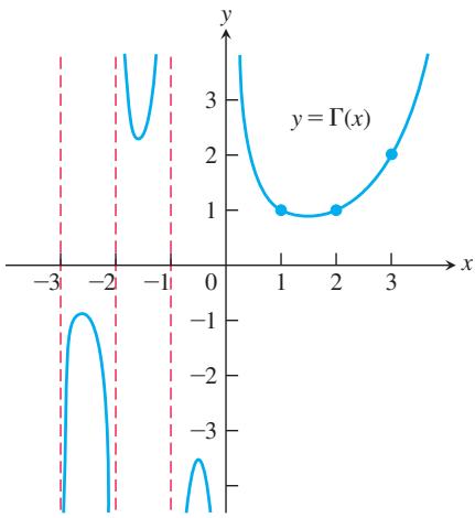
For each positive x, the number $Γ (𝑥)$ is the integral of $𝑡 𝑥 - 1 𝑒 - 𝑡$ with respect to t from 0 to $\infty$ . Figure 8.21 shows the graph of $Γ$ near the origin. You will see how to calculate $Γ (1 / 2)$ if you do Additional Exercise 23 in Chapter 14.

教材插图

FIGURE 8.21 Euler’s gamma function $Γ (𝑥)$ is a continuous function of $𝑥$ whose value at each positive integer $𝑛 + 1$ is $𝑛!$ . The defining integral formula for $Γ$ is valid only for $𝑥 > 0$ , but we can extend $Γ$ to negative noninteger values of $𝑥$ with the formula $Γ (𝑥) = (Γ (𝑥 + 1)) / 𝑥$ , which is the subject of Exercise 43.

If $𝑛$ is a nonnegative integer, then $Γ (𝑛 + 1) = 𝑛!$

a. Show that $Γ (1) = 1$ .

b. Then apply integration by parts to the integral for $Γ (𝑥 + 1)$ to show that $Γ (𝑥 + 1) = 𝑥 Γ (𝑥)$ . This gives

Γ (2) = 1 Γ (1) = 1 Γ (3) = 2 Γ (2) = 2 Γ (4) = 3 Γ (3) = 6 ⋮ Γ (𝑛 + 1) = 𝑛 Γ (𝑛) = 𝑛! (1)

c. Use mathematical induction to verify Equation (1) for every nonnegative integer $𝑛$ .

Stirling’s formula Scottish mathematician James Stirling (1692-1770) showed that

l i m 𝑥 \to \infty (𝑒 𝑥) 𝑥 \sqrt 𝑥 2 𝜋 Γ (𝑥) = 1,

so, for large x,

Γ (𝑥) = (𝑥 𝑒) 𝑥 \sqrt 2 𝜋 𝑥 (1 + 𝜀 (𝑥)) 𝜀 (𝑥) \to 0 a s 𝑥 \to \infty . (2)

Dropping $𝜀 (𝑥)$ leads to the approximation

$Γ (𝑥) \approx (𝑥 𝑒) 𝑥 \sqrt 2 𝜋 𝑥$ (Stirling’s formula).

(3)

a. Stirling’s approximation for $𝑛!$ Use Equation (3) and the fact that $𝑛! = 𝑛 Γ (𝑛)$ to show that $𝑛! \approx (𝑛 𝑒) 𝑛 \sqrt 2 𝑛 𝜋$ (Stirling’s approximation). (4)

As you will see if you do Exercise 114 in Section 9.1, Equation (4) leads to the approximation

𝑛 \sqrt 𝑛! \approx 𝑛 𝑒 . (5)

T b. Compare your calculator’s value for $𝑛!$ with the value given by Stirling’s approximation for $𝑛 = 10, 20, 30, \dots$ , as far as your calculator can go.

T c. A refinement of Equation (2) gives

Γ (𝑥) = (𝑥 𝑒) 𝑥 \sqrt 2 𝜋 𝑥 𝑒 1 / (12 𝑥) (1 + 𝜀 (𝑥))

Γ (𝑥) \approx (𝑥 𝑒) 𝑥 \sqrt 2 𝜋 𝑥 𝑒 1 / (12 𝑥),

which tells us that

𝑛! \approx (𝑛 𝑒) 𝑛 \sqrt 2 𝑛 𝜋 𝑒 1 / (12 𝑛) . (6)

Compare the values given for 10! by your calculator, Stirling’s approximation, and Equation (6).

CHAPTER 8 Technology Application Projects

Mathematica/Maple Projects

Projects can be found within MyLab Math.

• Riemann, Trapezoidal, and Simpson Approximations

Part I: Visualize the error involved in using Riemann sums to approximate the area under a curve.

Part II: Build a table of values and compute the relative magnitude of the error as a function of the step size $Δ 𝑥$ .

Part III: Investigate the effect of the derivative function on the error.

Parts IV and V: Trapezoidal Rule approximations.

Part VI: Simpson’s Rule approximations.

Games of Chance: Exploring the Monte Carlo Probabilistic Technique for Numerical Integration Graphically explore the Monte Carlo method for approximating definite integrals.
Computing Probabilities with Improper Integrals More explorations of the Monte Carlo method for approximating definite integrals.

教材插图

Infinite Sequences and Series

教材插图

OVERVIEW In this chapter we introduce the topic of infinite series. Such series give us precise ways to express many numbers and functions, both familiar and new, as arithmetic sums with infinitely many terms. For example, we will learn that

𝜋 4 = 1 - 13 + 15 - 17 + 19 - \dots

and

c o s 𝑥 = 1 - 𝑥 2 2 + 𝑥 4 24 - 𝑥 6 720 + 𝑥 8 40, 320 - \dots .

We need to develop a method to make sense of such expressions. Everyone knows how to add two numbers together, or even several. But how do you add together infinitely many numbers? Or, when adding together functions, how do you add infinitely many powers of x? In this chapter we answer these questions, which are part of the theory of infinite sequences and series. As with the differential and integral calculus, limits play a major role in the development of infinite series.

One common and important application of series occurs in making computations with complicated functions. A hard-to-compute function is replaced by an expression that looks like an “infinite degree polynomial,” an infinite series in powers of x, as we see with the cosine function given above. Using the first few terms of this infinite series can allow for highly accurate approximations of functions by polynomials, enabling us to work with more general functions than those we have encountered before. These new functions are commonly obtained as solutions to differential equations arising in important applications of mathematics to science and engineering.

The terms “sequence” and “series” are sometimes used interchangeably in spoken language. In mathematics, however, each has a distinct meaning. A sequence is a type of infinite list, whereas a series is an infinite sum. To understand the infinite sums described by series, we first must understand infinite sequences.

Chapter 8: Techniques of Integration

8.1 Using Basic Integration Formulas

EXERCISES 8.1

Assorted Integrations

8.2 Integration by Parts

Product Rule in Integral Form

Evaluating Definite Integrals by Parts

EXERCISES 8.2

Theory and Examples

8.3 Trigonometric Integrals

Products of Powers of Sines and Cosines

Eliminating Square Roots

Integrals of Powers of tan x and sec x

Products of Sines and Cosines

EXERCISES 8.3

8.4 Trigonometric Substitutions

Procedure for a Trigonometric Substitution

EXERCISES 8.4

Using Trigonometric Substitutions

Applications and Examples

8.5 Integration of Rational Functions by Partial Fractions

General Description of the Method

Method of Partial Fractions When 𝑓(𝑥)/𝑔(𝑥) Is Proper

Determining Coefficients by Differentiating

EXERCISES 8.5

Expanding Quotients into Partial Fractions

Repeated Linear Factors

Improper Fractions

Evaluating Integrals

Initial Value Problems

Applications and Examples

8.6 Integral Tables and Computer Algebra Systems

Integral Tables

Reduction Formulas

Integration with a CAS

Nonelementary Integrals

EXERCISES 8.6

Using Integral Tables

Substitution and Integral Tables

Applications

8.7 Numerical Integration

Approximating Integrals with the Midpoint Rule

Trapezoidal Approximations

Simpson’s Rule: Approximations Using Parabolas

Thomas Simpson (1720–1761)

Simpson’s Rule

Error Analysis

EXERCISES 8.7

Estimating Definite Integrals

I. Using the Midpoint Rule

II. Using the Trapezoidal Rule

III. Using Simpson’s Rule

Estimating the Number of Subintervals

Estimates with Numerical Data

Theory and Examples

Applications

8.8 Improper Integrals

Infinite Limits of Integration

Integrands with Vertical Asymptotes

Improper Integrals with a CAS

Tests for Convergence and Divergence

EXERCISES 8.8

Evaluating Improper Integrals

COMPUTER EXPLORATIONS

CHAPTER 8 Questions to Guide Your Review

CHAPTER 8 Practice Exercises

Integration by Parts

Partial Fractions

CHAPTER 8 Additional and Advanced Exercises

Evaluating Integrals

Applications

CHAPTER 8 Technology Application Projects

Mathematica/Maple Projects

Method of Partial Fractions When $𝑓 (𝑥) / 𝑔 (𝑥)$ Is Proper