Chapter 5: Integrals
OVERVIEW A great achievement of classical geometry was obtaining formulas for the areas and volumes of triangles, spheres, and cones. In this chapter we develop a method, called integration, to calculate the areas and volumes of more general shapes. The definite integral is the key tool in calculus for defining and calculating areas and volumes. We also use it to compute quantities such as the lengths of curved paths, probabilities, averages, energy consumption, the mass of an object, and the force against a dam’s floodgates.
Like the derivative, the definite integral is defined as a limit. The definite integral is a limit of increasingly fine approximations. The idea is to approximate a quantity (such as the area of a curvy region) by dividing it into many small pieces, each of which we can approximate by something simple (such as a rectangle). Summing the contributions of each of the simple pieces gives us an approximation to the original quantity. As we divide the region into more and more pieces, the approximation given by the sum of the pieces will generally improve, converging to the quantity we are measuring. We take a limit as the number of terms increases to infinity, and when the limit exists, the result is a definite integral. We develop this idea in Section 5.3.
We also show that the process of computing these definite integrals is closely connected to finding antiderivatives. This is one of the most important relationships in calculus; it gives us an efficient way to compute definite integrals, providing a simple and powerful method that eliminates the difficulty of directly computing limits of approximations. This connection is captured in the Fundamental Theorem of Calculus.
5.1 Area and Estimating with Finite Sums
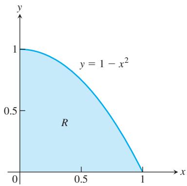
FIGURE 5.1 The area of the shaded region R cannot be found by a simple formula.
The basis for formulating definite integrals is the construction of approximations by finite sums. In this section we consider three examples of this process: finding the area under a graph, the distance traveled by a moving object, and the average value of a function. Although we have yet to define precisely what we mean by the area of a general region in the plane, or the average value of a function over a closed interval, we do have intuitive ideas of what these notions mean. We begin our approach to integration by approximating these quantities with simpler finite sums related to these intuitive ideas. We then consider what happens when we take more and more terms in the summation process. In subsequent sections we look at taking the limit of these sums as the number of terms goes to infinity, which leads to a precise definition of the definite integral.
Area
Suppose we want to find the area of the shaded region R that lies above the x-axis, below the graph of
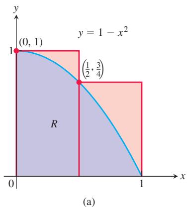
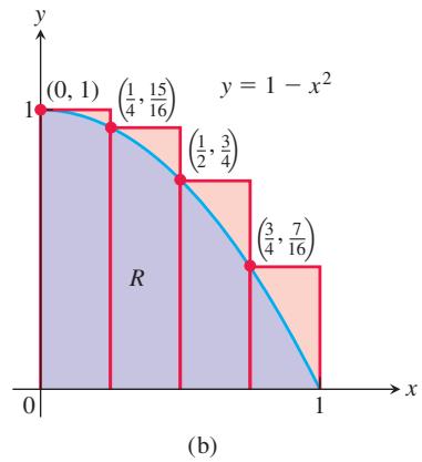
FIGURE 5.2 (a) We get an upper sum approximation of the area of R by using two rectangles containing R. (b) Four rectangles give a better upper sum approximation. Both estimates overshoot the true value for the area by the amount shaded in light red.
Unfortunately, there is no simple geometric formula for calculating the areas of general shapes having curved boundaries like the region R. How, then, can we find the area of R?
Although we do not yet have a method for determining the exact area of R, we can approximate it in a simple way. Figure 5.2a shows two rectangles that together contain the region R. Each rectangle has width 1/2 and they have heights 1 and 3/4 (left to right). The height of each rectangle is the maximum value of the function f in each subinterval. Because the function f is decreasing, the height is its value at the left endpoint of the subinterval of
This estimate is larger than the true area A since the two rectangles contain R. We say that 0.875 is an upper sum because it is obtained by taking the height of the rectangle corresponding to the maximum (uppermost) value of
which is still greater than A since the four rectangles contain R.
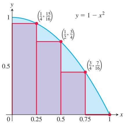
Suppose instead we use four rectangles contained inside the region R to estimate the area, as in Figure 5.3a. Each rectangle has width 1/4, as before, but the rectangles are shorter and lie entirely beneath the graph of f. The function
This estimate is smaller than the area A since the rectangles all lie inside of the region R. The true value of A lies somewhere between these lower and upper sums:
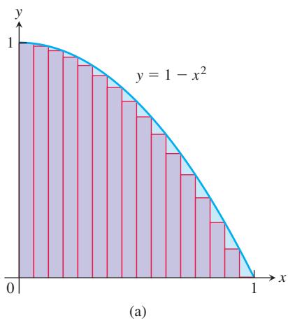
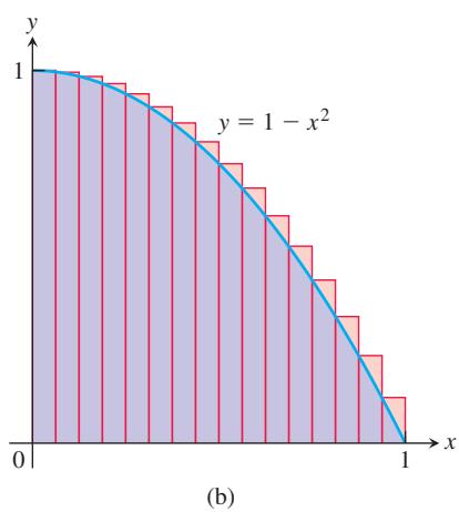
FIGURE 5.4 (a) A lower sum using 16 rectangles of equal width
(a)
(b)
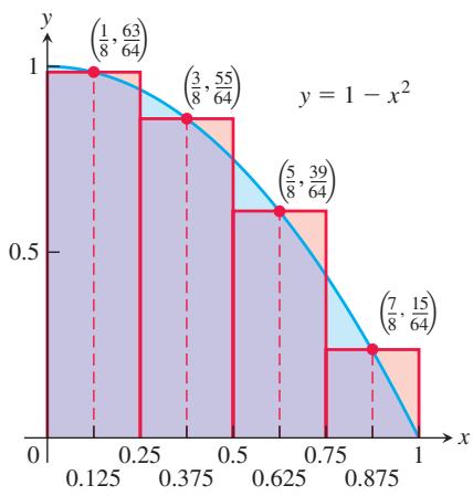
FIGURE 5.3 (a) Rectangles contained in R give a lower sum approximation for the area. This estimate undershoots the true value by the amount shaded in light blue. (b) The midpoint rule uses rectangles whose heights are the values of
Considering both lower and upper sum approximations gives us estimates for the area and a bound on the size of the possible error in these estimates since the true value of the area lies somewhere between them. Here the error cannot be greater than the difference 0.78125 - 0.53125 = 0.25.
Yet another estimate can be obtained by using rectangles whose heights are the values of f at the midpoints of the bases of the rectangles (Figure 5.3b). This method of estimation is called the midpoint rule for approximating the area. The midpoint rule gives an estimate that is between a lower sum and an upper sum, but it is not clear whether it overestimates or underestimates the true area. With four rectangles of width 1/4, as before, the midpoint rule estimates the area of R to be
In each of the sums that we computed, the interval
As we take more and more rectangles, with each rectangle thinner than before, it appears that these finite sums give better and better approximations to the true area of the region R.
Figure 5.4a shows a lower sum approximation for the area of R using 16 rectangles of equal width. The sum of their areas is 0.634765625, which appears close to the true area but is still somewhat smaller since the rectangles lie inside R.
Figure 5.4b shows an upper sum approximation using 16 rectangles of equal width. The sum of their areas is 0.697265625, which is somewhat larger than the true area because the rectangles taken together contain R. The midpoint rule for 16 rectangles gives a total area approximation of 0.6669921875, but it is not immediately clear whether this estimate is larger or smaller than the true area.
Table 5.1 shows the values of upper and lower sum approximations to the area of R, using up to 1000 rectangles. The values of these approximations appear to be approaching 2/3. In Section 5.2 we will see how to get an exact value of the area of regions such as R by taking a limit as the base width of each rectangle goes to zero and the number of rectangles goes to infinity. With the techniques developed there, we will be able to show that the area of R is exactly 2/3.
TABLE 5.1 Finite approximations for the area of R
| Number of subintervals | Lower sum | Midpoint sum | Upper sum |
| 2 | 0.375 | 0.6875 | 0.875 |
| 4 | 0.5313 | 0.6719 | 0.7813 |
| 16 | 0.6348 | 0.6670 | 0.6973 |
| 50 | 0.6566 | 0.6667 | 0.6766 |
| 100 | 0.66165 | 0.666675 | 0.67165 |
| 1000 | 0.6661665 | 0.66666675 | 0.6671665 |
Distance Traveled
Suppose we know the velocity function
If we know the velocity at a collection of times
and add the results across
Suppose the subdivided interval looks like
with the subintervals all of equal length
where n is the total number of subintervals. This sum is only an approximation to the true distance D, but the approximation increases in accuracy as we take more and more subintervals.
EXAMPLE 1 The velocity function of a projectile fired straight into the air is
Solution We explore the results for different numbers of subintervals and different choices of evaluation points. Notice that
(a) Three subintervals of length 1, with f evaluated at left endpoints giving an upper sum:
With f evaluated at t = 0, 1, and 2, we have
(b) Three subintervals of length 1, with f evaluated at right endpoints giving a lower sum:
With
(c) With six subintervals of length 1/2, we get
These estimates give an upper sum using left endpoints:
As we can see in Table 5.2, the left-endpoint upper sums approach the true value 435.9 from above, whereas the right-endpoint lower sums approach it from below. The true value lies between these upper and lower sums. The magnitude of the error in the closest entry is 0.23, a small percentage of the true value.
It is reasonable to conclude from the table’s last entries that the projectile rose about 436 m during its first 3 sec of flight.
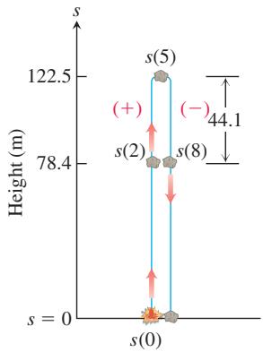
FIGURE 5.5 The rock in Example 2. The height s = 78.4 m is reached at t = 2 s and t = 8 s. The rock falls 44.1 m from its maximum height when t = 8.
TABLE 5.2 Travel-distance estimates
| Number of subintervals | Length of each subinterval | Upper sum | Lower sum |
| 3 | 1 | 450.6 | 421.2 |
| 6 | 1/2 | 443.25 | 428.55 |
| 12 | 1/4 | 439.58 | 432.23 |
| 24 | 1/8 | 437.74 | 434.06 |
| 48 | 1/16 | 436.82 | 434.98 |
| 96 | 1/32 | 436.36 | 435.44 |
| 192 | 1/64 | 436.13 | 435.67 |
Displacement Versus Distance Traveled
If an object with position function
To see why using the velocity function in the summation process gives an estimate of the displacement, partition the time interval
The change is positive if
In either case, the distance traveled by the object during the subinterval is about
The total distance traveled over the time interval is approximately the sum
We will revisit these ideas in Section 5.4.
EXAMPLE 2 In Example 4 in Section 3.4, we analyzed the motion of a heavy rock blown straight up by a dynamite blast. In that example, we found the velocity of the rock at time t was
Solution If we follow a procedure like the one presented in Example 1, using the velocity function
TABLE 5.3 Velocity function
| t | v(t) | t | v(t) |
| 0 | 49 | 4.5 | 4.9 |
| 0.5 | 44.1 | 5.0 | 0 |
| 1.0 | 39.2 | 5.5 | -4.9 |
| 1.5 | 34.3 | 6.0 | -9.8 |
| 2.0 | 29.4 | 6.5 | -14.7 |
| 2.5 | 24.5 | 7.0 | -19.6 |
| 3.0 | 19.6 | 7.5 | -24.5 |
| 3.5 | 14.7 | 8.0 | -29.4 |
| 4.0 | 9.8 |
44.1 m ending at a height of 78.4 m at time t = 8. The velocity
On the other hand, if we use the speed
As an illustration of our discussion, we subdivide the interval
Using
Using
If we take more and more subintervals of
TABLE 5.4 Travel estimates for a rock blown straight up during the time interval [0, 8]
| Number of subintervals | Length of each subinterval | Displacement | Total distance |
| 16 | 1/2 | 58.8 | 161.7 |
| 32 | 1/4 | 68.6 | 164.15 |
| 64 | 1/8 | 73.5 | 165.375 |
| 128 | 1/16 | 75.95 | 165.9875 |
| 256 | 1/32 | 77.175 | 166.29375 |
| 512 | 1/64 | 77.7875 | 166.446875 |
Average Value of a Nonnegative Continuous Function
The average value of a collection of n numbers
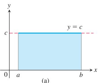
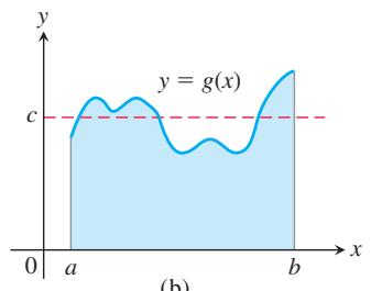
FIGURE 5.6 (a) The average value of
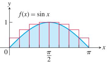
FIGURE 5.7 Approximating the area under
When a function is constant, this question is easy to answer. A function with constant value c on an interval
What if we want to find the average value of a nonconstant function, such as the function g in Figure 5.6b? We can think of this graph as a snapshot of the height of some water that is sloshing around in a tank between enclosing walls at x = a and x = b. As the water moves, its height over each point changes, but its average height remains the same. To get the average height of the water, we let it settle down until it is level and its height is constant. The resulting height c equals the area under the graph of g divided by b - a. We are led to define the average value of a nonnegative function on an interval
EXAMPLE 3 Estimate the average value of the function
Solution Looking at the graph of
We do not have a simple way to determine the area, so we approximate it with finite sums. To get an upper sum approximation, we add the areas of eight rectangles of equal width
To estimate the average value of
Since we used an upper sum to approximate the area, this estimate is greater than the actual average value of
TABLE 5.5 Average value of sin x on
| Number of subintervals | Upper sum estimate |
| 8 | 0.75342 |
| 16 | 0.69707 |
| 32 | 0.65212 |
| 50 | 0.64657 |
| 100 | 0.64161 |
| 1000 | 0.63712 |
As before, we could just as well have used rectangles lying under the graph of
Summary
The area under the graph of a positive function, the distance traveled by a moving object that doesn’t change direction, and the average value of a nonnegative function
The choices for the
EXERCISES 5.1
Area
In Exercises 1–4, apply finite approximations to estimate the area under the graph of the function using
a. a lower sum with two rectangles of equal width.
b. a lower sum with four rectangles of equal width.
c. an upper sum with two rectangles of equal width.
d. an upper sum with four rectangles of equal width.
-
𝑓 ( 𝑥 ) = 𝑥 2 𝑥 = 0 𝑥 = 1 -
𝑓 ( 𝑥 ) = 𝑥 3 -
𝑓 ( 𝑥 ) = 1 / 𝑥 -
𝑓 ( 𝑥 ) = 4 − 𝑥 2
Using rectangles, each of whose height is given by the value of the function at the midpoint of the rectangle’s base (the midpoint rule), estimate the area under the graphs of the following functions, using first two and then four rectangles.
-
𝑓 ( 𝑥 ) = 𝑥 2 -
𝑓 ( 𝑥 ) = 𝑥 3 -
𝑓 ( 𝑥 ) = 1 / 𝑥 -
𝑓 ( 𝑥 ) = 4 − 𝑥 2
Distance
- Distance traveled The accompanying table shows the velocity of a model train engine moving along a track for 10 s. Estimate the distance traveled by the engine using 10 subintervals of length 1 with a. left-endpoint values.
b. right-endpoint values.
| Time (s) | Velocity (cm/s) | Time (s) | Velocity (cm/s) |
| 0 | 0 | 6 | 11 |
| 1 | 12 | 7 | 6 |
| 2 | 22 | 8 | 2 |
| 3 | 10 | 9 | 6 |
| 4 | 5 | 10 | 0 |
| 5 | 13 |
- Distance traveled upstream You are sitting on the bank of a tidal river watching the incoming tide carry a bottle upstream. You record the velocity of the flow every 5 minutes for an hour, with the results shown in the accompanying table. About how far upstream did the bottle travel during that hour? Find an estimate using 12 subintervals of length 5 with
a. left-endpoint values.
b. right-endpoint values.
| Time (min) | Velocity (m/s) | Time (min) | Velocity (m/s) |
| 0 | 1 | 35 | 1.2 |
| 5 | 1.2 | 40 | 1.0 |
| 10 | 1.7 | 45 | 1.8 |
| 15 | 2.0 | 50 | 1.5 |
| 20 | 1.8 | 55 | 1.2 |
| 25 | 1.6 | 60 | 0 |
| 30 | 1.4 |
- Length of a road You and a companion are about to drive a twisty stretch of dirt road in a car whose speedometer works but whose odometer (kilometer counter) is broken. To find out how long this particular stretch of road is, you record the car’s velocity at 10-second intervals, with the results shown in the accompanying table. Estimate the length of the road using
a. left-endpoint values.
b. right-endpoint values.
| Time (s) | Velocity (converted to m/s) (36 km/h = 10 m/s) | Time (s) | Velocity (converted to m/s) (30 km/h = 10 m/s) |
| 0 | 0 | 70 | 5 |
| 10 | 15 | 80 | 7 |
| 20 | 5 | 90 | 12 |
| 30 | 12 | 100 | 15 |
| 40 | 10 | 110 | 10 |
| 50 | 15 | 120 | 12 |
| 60 | 12 |
- Distance from velocity data The accompanying table gives data for the velocity of a vintage sports car accelerating from 0 to 228 km/h in 36 s (10 thousandths of an hour).
| Time (h) | Velocity (km/h) | Time (h) | Velocity (km/h) |
| 0.0 | 0 | 0.006 | 187 |
| 0.001 | 64 | 0.007 | 201 |
| 0.002 | 100 | 0.008 | 212 |
| 0.003 | 132 | 0.009 | 220 |
| 0.004 | 154 | 0.010 | 228 |
| 0.005 | 174 |
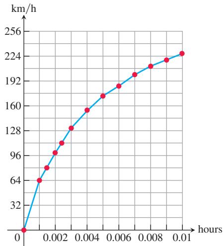
a. Use rectangles to estimate how far the car traveled during the 36 s it took to reach 228 km/h.
b. Roughly how many seconds did it take the car to reach the halfway point? About how fast was the car going then?
- Free fall with air resistance An object is dropped straight down from a helicopter. The object falls faster and faster but its acceleration (rate of change of its velocity) decreases over time because of air resistance. The acceleration is measured in m/s
2
| t | 0 | 1 | 2 | 3 | 4 | 5 |
| a | 9.8 | 5.944 | 3.605 | 2.187 | 1.326 | 0.805 |
a. Find an upper estimate for the speed when t = 5.
b. Find a lower estimate for the speed when t = 5.
c. Find an upper estimate for the distance fallen when t = 3.
- Distance traveled by a projectile An object is shot straight upward from sea level with an initial velocity of 122.5 m/s.
a. Assuming that gravity is the only force acting on the object, give an upper estimate for its velocity after 5 s have elapsed. Use
b. Find a lower estimate for the height attained after 5 s.
Average Value of a Function
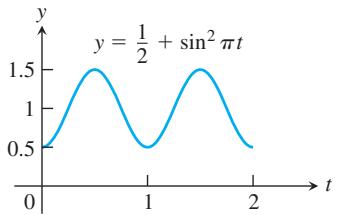
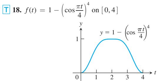
In Exercises 15–18, use a finite sum to estimate the average value of f on the given interval by partitioning the interval into four subintervals of equal length and evaluating f at the subinterval midpoints.
𝑓 ( 𝑡 ) = ( 1 / 2 ) + s i n 2 𝜋 𝑡 o n [ 0 , 2 ]
T 18.
Estimations
- Water pollution Oil is leaking out of a tanker damaged at sea. The damage to the tanker is worsening as evidenced by the increased leakage each hour, recorded in the following table.
| Time (h) | 0 | 1 | 2 | 3 | 4 |
| Leakage (L/h) | 50 | 70 | 97 | 136 | 190 |
| Time (h) | 5 | 6 | 7 | 8 | |
| Leakage (L/h) | 265 | 369 | 516 | 720 |
a. Give an upper and a lower estimate of the total quantity of oil that has escaped after 5 hours.
b. Repeat part (a) for the quantity of oil that has escaped after 8 hours.
c. The tanker continues to leak 720 L/h after the first 8 hours. If the tanker originally contained 25,000 L of oil, approximately how many more hours will elapse in the worst case before all the oil has spilled? In the best case?
- Air pollution A power plant generates electricity by burning oil. Pollutants produced as a result of the burning process are removed by scrubbers in the smokestacks. Over time, the scrubbers become less efficient and eventually they must be replaced when the amount of pollution released exceeds government standards. Measurements are taken at the end of each month determining the rate at which pollutants are released into the atmosphere, recorded as follows.
| Month | Jan | Feb | Mar | Apr | May | Jun |
| Pollutant release rate (tons/day) | 0.20 | 0.25 | 0.27 | 0.34 | 0.45 | 0.52 |
| Month | Jul | Aug | Sep | Oct | Nov | Dec |
| Pollutant release rate (tons/day) | 0.63 | 0.70 | 0.81 | 0.85 | 0.89 | 0.95 |
a. Assuming a 30-day month and that new scrubbers allow only 0.05 ton/day to be released, give an upper estimate of the total tonnage of pollutants released by the end of June. What is a lower estimate?
b. In the best case, approximately when will a total of 125 tons of pollutants have been released into the atmosphere?
- Inscribe a regular n-sided polygon inside a circle of radius 1 and compute the area of the polygon for the following values of n: a. 4 (square) b. 8 (octagon) c. 16
d. Compare the areas in parts (a), (b), and (c) with the area inside the circle.
- (Continuation of Exercise 21.)
a. Inscribe a regular n-sided polygon inside a circle of radius 1 and compute the area of one of the n congruent triangles formed by drawing radii to the vertices of the polygon.
b. Compute the limit of the area of the inscribed polygon as
c. Repeat the computations in parts (a) and (b) for a circle of radius r.
COMPUTER EXPLORATIONS
In Exercises 23–26, use a CAS to perform the following steps.
a. Plot the functions over the given interval.
b. Subdivide the interval into n = 100, 200, and 1000 subintervals of equal length and evaluate the function at the midpoint of each subinterval.
c. Compute the average value of the function values generated in part (b).
d. Solve the equation
5.2 Sigma Notation and Limits of Finite Sums
While estimating with finite sums in Section 5.1, we encountered sums that had many terms (up to 1000 terms in Table 5.1). In this section we introduce a notation for sums that have a large number of terms. After describing this notation and its properties, we consider what happens as the number of terms in a sum approaches infinity.
Finite Sums and Sigma Notation
Sigma notation enables us to write a sum with many terms in the compact form
The Greek letter
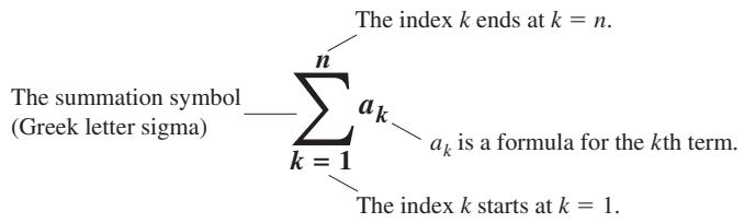
Thus we can write the sum of the squares of the numbers 1 through 11 as
and the sum of
The starting index does not have to be 1; it can be any integer.
EXAMPLE 1
| A sum in sigma notation | The sum written out, one term for each value of | The value of the sum |
| 15 | ||
EXAMPLE 2 Express the sum
Solution The formula generating the terms depends on what we choose the lower limit of summation to be, but the terms generated remain the same. It is often simplest to choose the starting index to be k = 0 or k = 1, but we can start with any integer.
When we have a sum such as
we can rearrange its terms to form two sums:
This illustrates a general rule for finite sums:
This and three other rules are given below. Proofs of these rules can be obtained using mathematical induction (see Appendix A.3).
Algebra Rules for Finite Sums
- Sum Rule:
- Difference Rule:
- Constant Multiple Rule:
(Any number
- Constant Value Rule:
(Any number
EXAMPLE 3 We demonstrate the use of the algebra rules.
Difference Rule and Constant Multiple Rule
Constant Multiple Rule
HISTORICAL BIOGRAPHY
Carl Friedrich Gauss
(1777-1855)
Gauss was born in Brunswick, Germany. The list of Gauss’s accomplishments in science and mathematics is astonishing, ranging from the invention of the electric telegraph (with Wilhelm Weber in 1833) to the development of a theory of planetary orbits and the development of an accurate theory of non-Euclidean geometry.
To know more, visit the companion Website.
Sum Rule
Constant Value Rule
Constant Value Rule
(1/n is constant)
Over the years, people have discovered a variety of formulas for the values of finite sums. The most famous of these are the formula for the sum of the first n positive integers (Gauss is said to have discovered it at age 8) and the formulas for the sums of the squares and cubes of the first n positive integers.
EXAMPLE 4 Show that the sum of the first n positive integers is
Solution The formula tells us that the sum of the first 4 positive integers is
Addition verifies this prediction:
To prove the formula in general, we write out the terms in the sum twice, once forward and once backward.
If we add the two terms in the first column we get
Formulas for the sums of the squares and cubes of the first n positive integers are proved using mathematical induction (see Appendix A.3). We state them here.
Sum of the first
Sum of the first
Limits of Finite Sums
The finite sum approximations that we considered in Section 5.1 became more accurate as the number of terms increased and the subinterval widths (lengths) narrowed. The next example shows how to calculate a limiting value as the widths of the subintervals go to zero and the number of subintervals grows to infinity.
EXAMPLE 5 Find the limiting value of lower sum approximations to the area of the region R below the graph of
Solution We compute a lower sum approximation using n rectangles of equal width
Each subinterval has width
We write this in sigma notation and simplify,
We have obtained an expression for the lower sum that holds for any n. Taking the limit of this expression as
The lower sum approximations converge to 2/3. A similar calculation shows that the upper sum approximations also converge to 2/3. Any finite sum approximation
HISTORICAL BIOGRAPHY
Georg Friedrich Bernhard Riemann (1826–1866)
Riemann was born in Hanover, Germany. His doctorate was obtained under the direction of Gauss in the theory of complex variables. He also worked with physicist Wilhelm Weber. He introduced the foundational ideas of differential geometry and contributed to dynamics, non-Euclidean geometry, and computational physics. To know more, visit the companion Website.
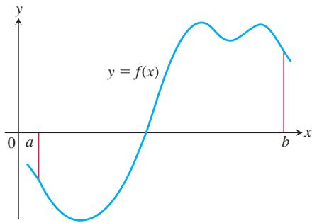
FIGURE 5.8 A typical continuous function
Riemann Sums
The theory of limits of finite approximations was made precise by the German mathematician Bernhard Riemann. We now introduce the notion of a Riemann sum, which underlies the theory of the definite integral that will be presented in the next section.
We begin with an arbitrary bounded function f defined on a closed interval
To make the notation consistent, we set
The set of all of these points,
is called a partition of
The partition P divides
HISTORICAL BIOGRAPHY Richard Dedekind (1831–1916)
Dedekind grew up in Germany and in 1850 entered the University of Gottingen. There he studied with Bernhard Riemann and Carl Gauss. Like Gauss, Dedekind preferred to study the theoretical aspects of number theory. His work on irrational numbers gave the subject a logical foundation.
To know more, visit the companion Website.
The first of these subintervals is

The width of the first subinterval

If all n subintervals have equal width, then their common width, which we call
In each subinterval we select some point. The point chosen in the kth subinterval
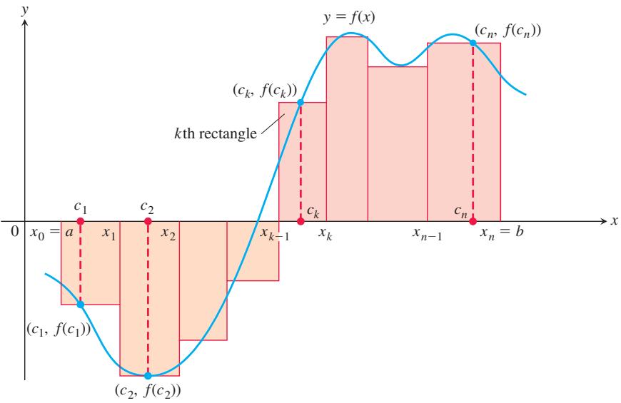
FIGURE 5.9 The rectangles approximate the region between the graph of the function
On each subinterval we form the product
Finally, we sum all these products to get
The sum
(a)
(b)
Similar formulas can be obtained if instead we choose
In the cases in which the subintervals all have equal width
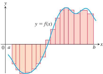
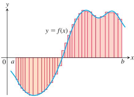
FIGURE 5.10 The curve of Figure 5.9 with rectangles from finer partitions of
EXAMPLE 6 The set

The lengths of the subintervals are
Any Riemann sum associated with a partition of a closed interval
EXERCISES 5.2
Sigma Notation
Write the sums in Exercises 1–6 without sigma notation. Then evaluate them.
-
∑ 2 𝑘 = 1 6 𝑘 𝑘 + 1 -
∑ 3 𝑘 = 1 𝑘 − 1 𝑘 -
∑ 4 𝑘 = 1 c o s 𝑘 𝜋 -
∑ 5 𝑘 = 1 s i n 𝑘 𝜋 -
∑ 3 𝑘 = 1 ( − 1 ) 𝑘 + 1 s i n 𝜋 𝑘 -
∑ 4 𝑘 = 1 ( − 1 ) 𝑘 c o s 𝑘 𝜋 -
Which of the following express
1 + 2 + 4 + 8 + 1 6 + 3 2 ∑ 6 𝑘 = 1 2 𝑘 − 1 ∑ 5 𝑘 = 0 2 𝑘 ∑ 4 𝑘 = − 1 2 𝑘 + 1 -
Which of the following express
1 − 2 + 4 − 8 + 1 6 − 3 2 ∑ 6 𝑘 = 1 ( − 2 ) 𝑘 − 1 ∑ 5 𝑘 = 0 ( − 1 ) 𝑘 2 𝑘 ∑ 3 𝑘 = − 2 ( − 1 ) 𝑘 + 1 2 𝑘 + 2 -
Which formula is not equivalent to the other two? a.
∑ 4 𝑘 = 2 ( − 1 ) 𝑘 − 1 𝑘 − 1 ∑ 2 𝑘 = 0 ( − 1 ) 𝑘 𝑘 + 1 ∑ 1 𝑘 = − 1 ( − 1 ) 𝑘 𝑘 + 2 -
Which formula is not equivalent to the other two? a.
∑ 4 𝑘 = 1 ( 𝑘 − 1 ) 2 ∑ 3 𝑘 = − 1 ( 𝑘 + 1 ) 2 ∑ − 1 𝑘 = − 3 𝑘 2
Express the sums in Exercises 11–16 in sigma notation. The form of your answer will depend on your choice for the starting index.
11.
-
1 + 4 + 9 + 1 6 -
1 2 + 1 4 + 1 8 + 1 1 6 -
2 + 4 + 6 + 8 + 1 0 -
1 − 1 2 + 1 3 − 1 4 + 1 5 -
− 1 5 + 2 5 − 3 5 + 4 5 − 5 5
Values of Finite Sums
- Suppose that
∑ 𝑛 𝑘 = 1 𝑎 𝑘 = − 5 ∑ 𝑛 𝑘 = 1 𝑏 𝑘 = 6 ∑ 𝑛 𝑘 = 1 3 𝑎 𝑘 ∑ 𝑛 𝑘 = 1 𝑏 𝑘 6 ∑ 𝑛 𝑘 = 1 ( 𝑎 𝑘 + 𝑏 𝑘 )
d.
- Suppose that
∑ 𝑛 𝑘 = 1 𝑎 𝑘 = 0 ∑ 𝑛 𝑘 = 1 𝑏 𝑘 = 1 ∑ 𝑛 𝑘 = 1 8 𝑎 𝑘 ∑ 𝑛 𝑘 = 1 2 5 0 𝑏 𝑘 ∑ 𝑛 𝑘 = 1 ( 𝑎 𝑘 + 1 ) ∑ 𝑛 𝑘 = 1 ( 𝑏 𝑘 − 1 )
Evaluate the sums in Exercises 19–36.
-
a.
∑ 1 0 𝑘 = 1 𝑘 ∑ 1 0 𝑘 = 1 𝑘 2 ∑ 1 0 𝑘 = 1 𝑘 3 -
a.
∑ 1 3 𝑘 = 1 𝑘 ∑ 1 3 𝑘 = 1 𝑘 2 ∑ 1 3 𝑘 = 1 𝑘 3 -
∑ 7 𝑘 = 1 ( − 2 𝑘 ) -
∑ 5 𝑘 = 1 𝜋 𝑘 1 5 -
∑ 6 𝑘 = 1 ( 3 − 𝑘 2 ) -
∑ 6 𝑘 = 1 ( 𝑘 2 − 5 ) -
∑ 5 𝑘 = 1 𝑘 ( 3 𝑘 + 5 ) -
∑ 7 𝑘 = 1 𝑘 ( 2 𝑘 + 1 ) -
∑ 5 𝑘 = 1 𝑘 3 2 2 5 + ( ∑ 5 𝑘 = 1 𝑘 ) 3 -
( ∑ 7 𝑘 = 1 𝑘 ) 2 − ∑ 7 𝑘 = 1 𝑘 3 4 -
a.
∑ 7 𝑘 = 1 3 ∑ 5 0 0 𝑘 = 1 7 ∑ 2 6 4 𝑘 = 3 1 0 -
a.
∑ 3 6 𝑘 = 9 𝑘 ∑ 1 7 𝑘 = 3 𝑘 2 ∑ 7 1 𝑘 = 1 8 𝑘 ( 𝑘 − 1 ) -
a.
∑ 𝑛 𝑘 = 1 4 ∑ 𝑛 𝑘 = 1 𝑐 ∑ 𝑛 𝑘 = 1 ( 𝑘 − 1 )
5.3 The Definite Integral
-
a.
∑ 𝑛 𝑘 = 1 ( 1 𝑛 + 2 𝑛 ) ∑ 𝑛 𝑘 = 1 𝑐 𝑛 ∑ 𝑛 𝑘 = 1 𝑘 𝑛 2 -
∑ 5 0 𝑘 = 1 [ ( 𝑘 + 1 ) 2 − 𝑘 2 ] ∑ 2 0 𝑘 = 2 [ s i n ( 𝑘 − 1 ) − s i n 𝑘 ] -
∑ 3 0 𝑘 = 7 ( √ 𝑘 − 4 − √ 𝑘 − 3 ) -
∑ 4 0 𝑘 = 1 1 𝑘 ( 𝑘 + 1 ) 1 𝑘 ( 𝑘 + 1 ) = 1 𝑘 − 1 𝑘 + 1
Riemann Sums
In Exercises 37–40, graph each function
-
𝑓 ( 𝑥 ) = 𝑥 2 − 1 , [ 0 , 2 ] 𝑓 ( 𝑥 ) = − 𝑥 2 , [ 0 , 1 ] -
𝑓 ( 𝑥 ) = s i n 𝑥 , [ − 𝜋 , 𝜋 ] -
𝑓 ( 𝑥 ) = s i n 𝑥 + 1 , [ − 𝜋 , 𝜋 ] -
Find the norm of the partition
𝑃 = { 0 , 1 . 2 , 1 . 5 , 2 . 3 , 2 . 6 , 3 } -
Find the norm of the partition
𝑃 = { − 2 , − 1 . 6 , − 0 . 5 , 0 , 0 . 8 , 1 }
Limits of Riemann Sums
For the functions in Exercises 43–50, find a formula for the Riemann sum obtained by dividing the interval
-
𝑓 ( 𝑥 ) = 1 − 𝑥 2 -
𝑓 ( 𝑥 ) = 2 𝑥 -
𝑓 ( 𝑥 ) = 𝑥 2 + 1 -
𝑓 ( 𝑥 ) = 3 𝑥 2 -
𝑓 ( 𝑥 ) = 𝑥 + 𝑥 2 -
𝑓 ( 𝑥 ) = 3 𝑥 + 2 𝑥 2 -
𝑓 ( 𝑥 ) = 2 𝑥 3 -
𝑓 ( 𝑥 ) = 𝑥 2 − 𝑥 3 [ − 1 , 0 ]
In this section we consider the limit of general Riemann sums as the norm of the partitions of a closed interval
Definition of the Definite Integral
The definition of the definite integral is based on the fact that for some functions, as the norm of the partitions of
DEFINITION Let
be a function defined on a closed interval 𝑓 ( 𝑥 ) . We say that a number [ 𝑎 , 𝑏 ] is the definite integral of 𝐽 over 𝑓 and that [ 𝑎 , 𝑏 ] is the limit of the Riemann sums 𝐽 if the following condition is satisfied: ∑ 𝑛 𝑘 = 1 𝑓 ( 𝑐 𝑘 ) Δ 𝑥 𝑘 Given any number
, there is a corresponding number 𝜀 > 0 such that for every partition 𝛿 > 0 of 𝑃 = { 𝑥 0 , 𝑥 1 , … , 𝑥 𝑛 } with [ 𝑎 , 𝑏 ] and any choice of | | 𝑃 | | < 𝛿 in 𝑐 𝑘 , we have [ 𝑥 𝑘 − 1 , 𝑥 𝑘 ] ∣ 𝑛 ∑ 𝑘 = 1 𝑓 ( 𝑐 𝑘 ) Δ 𝑥 𝑘 − 𝐽 ∣ < 𝜀 . The definition involves a limiting process in which the norm of the partition goes to zero. When this limit exists, the function
is said to be integrable over 𝑓 . [ 𝑎 , 𝑏 ]
We have many choices for a partition P with norm going to zero, and many choices of points
and we say that the definite integral exists.
Leibniz introduced a notation for the definite integral that captures its construction as a limit of Riemann sums. He envisioned the finite sums
If the definite integral exists, then instead of writing J, we write
We read this as “the integral from a to b of f of x dee x” or sometimes as “the integral from a to b of f of x with respect to x.” The component parts in the integral symbol also have names:
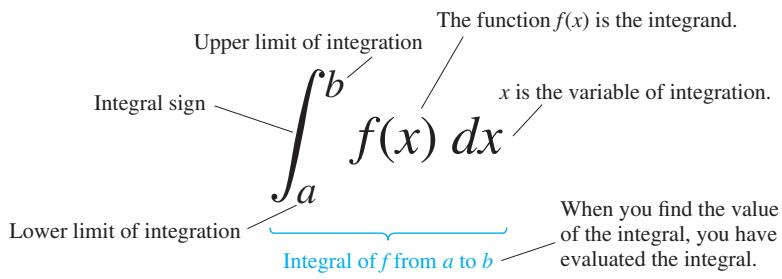
When the definite integral exists, we say that the Riemann sums of
If we choose all the subintervals in a partition to have equal width
where
If we pick the point
The Definite Integral as a Limit of Riemann Sums with Equal-Width Subintervals
Equation (1) gives an explicit formula that can be used to compute definite integrals. When the definite integral exists, the Riemann sums coming from other choices of partitions and locations of points
The value of the definite integral of a function over any particular interval depends on the function, not on the letter we choose to represent its independent variable. If we decide to use t or u instead of x, we simply write the integral as
No matter how we write the integral, it is still the same number, the limit of the Riemann sums as the norm of the partition approaches zero. Since it does not matter what letter we use, the variable of integration is called a dummy variable. In the three integrals given above, the dummy variables are t, u, and x.
Integrable and Nonintegrable Functions
Not every function defined over a closed interval
THEOREM 1—Continuous Functions Are Integrable If a function
The idea behind Theorem 1 for continuous functions is given in Exercises 86 and 87. Briefly, when
For integrability to fail, a function needs to be sufficiently discontinuous that the region between its graph and the x-axis cannot be approximated well by increasingly thin rectangles. Our first example is a function that is not integrable over a closed interval.
EXAMPLE 1 The function
has no Riemann integral over
If we choose a partition
As the norm of the partition approaches 0, these upper sum approximations converge to 1 (because each approximation is equal to 1).
On the other hand, we could pick the
These lower sum approximations converge to 0 as the norm of the partition converges to 0 (because they each equal 0).
Thus making different choices for the points
Theorem 1 says nothing about how to calculate definite integrals. A method of calculation will be developed in Section 5.4, through a connection of definite integrals to antiderivatives. Meanwhile, finite approximations can be used to calculate an approximation for a definite integral.
The Midpoint Rule
When setting up a Riemann sum
we have many options on how to choose a partition and where to choose a point
With these choices,
Midpoint Rule for Approximating a Definite Integral
EXAMPLE 2 Approximate
Solution The five intervals of the partition are
The midpoint rule becomes more powerful when we can combine it with an error bound that tells us how close the approximation it gives with n intervals is to the integral. In Chapter 8 we will examine error bounds in approximations of integrals.
Properties of Definite Integrals
In defining
It is convenient to have a definition for the integral over
TABLE 5.6 Rules satisfied by definite integrals
-
Order of Integration:
∫ 𝑎 𝑏 𝑓 ( 𝑥 ) 𝑑 𝑥 = − ∫ 𝑏 𝑎 𝑓 ( 𝑥 ) 𝑑 𝑥 -
Zero Width Interval:
∫ 𝑎 𝑎 𝑓 ( 𝑥 ) 𝑑 𝑥 = 0 -
Constant Multiple:
∫ 𝑏 𝑎 𝑘 𝑓 ( 𝑥 ) 𝑑 𝑥 = 𝑘 ∫ 𝑏 𝑎 𝑓 ( 𝑥 ) 𝑑 𝑥
Any constant
-
Sum and Difference:
∫ 𝑏 𝑎 ( 𝑓 ( 𝑥 ) ± 𝑔 ( 𝑥 ) ) 𝑑 𝑥 = ∫ 𝑏 𝑎 𝑓 ( 𝑥 ) 𝑑 𝑥 ± ∫ 𝑏 𝑎 𝑔 ( 𝑥 ) 𝑑 𝑥 -
Additivity:
∫ 𝑐 𝑎 𝑓 ( 𝑥 ) 𝑑 𝑥 + ∫ 𝑏 𝑐 𝑓 ( 𝑥 ) 𝑑 𝑥 = ∫ 𝑏 𝑎 𝑓 ( 𝑥 ) 𝑑 𝑥 [ 𝑎 , 𝑐 ] ∪ [ 𝑐 , 𝑏 ] = [ 𝑎 , 𝑏 ] -
Max-Min Inequality: If f has maximum value max f and minimum value
min
- Domination: If
𝑓 ( 𝑥 ) ≥ 𝑔 ( 𝑥 ) [ 𝑎 , 𝑏 ] ∫ 𝑏 𝑎 𝑓 ( 𝑥 ) 𝑑 𝑥 ≥ ∫ 𝑏 𝑎 𝑔 ( 𝑥 ) 𝑑 𝑥
If
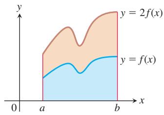
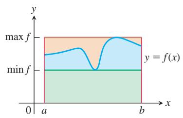
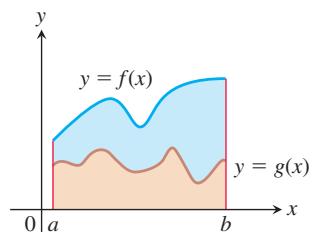
Theorem 2 states some basic properties of integrals, including the two just discussed. These properties, listed in Table 5.6, are very useful for computing integrals. We will refer to them repeatedly to simplify our calculations. Rules 2 through 7 have geometric interpretations, which are shown in Figure 5.11. The graphs in these figures show only positive functions, but the rules apply to general integrable functions, which could take both positive and negative values.
THEOREM 2 When f and g are integrable over the interval
Rules 1 and 2 are definitions, but Rules 3 to 7 of Table 5.6 must be proved. Below we give a proof of Rule 6. Similar proofs can be given to verify the other properties in Table 5.6.
Proof of Rule 6 Rule 6 says that the integral of f over
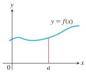
(a) Zero Width Interval:
(b) Constant Multiple:
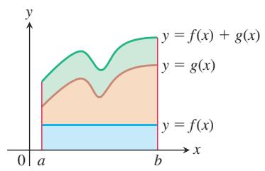
(c) Sum: (areas add)
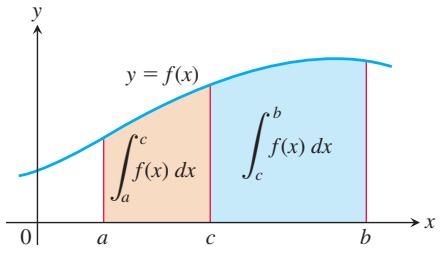
(d) Additivity for Definite Integrals:
(e) Max-Min Inequality:
(f) Domination:
FIGURE 5.11 Geometric interpretations of Rules 2–7 in Table 5.6.
In short, all Riemann sums for
Hence their limit, which is the integral, satisfies the same inequalities.
EXAMPLE 3 To illustrate some of the rules, we suppose that
Then
Rule 1
EXAMPLE 4 Show that the value of
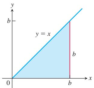
FIGURE 5.12 The region in Example 5 is a triangle.
Area Under the Graph of a Nonnegative Function
We now return to the problem that started this chapter, which is defining what we mean by the area of a region having a curved boundary. In Section 5.1 we approximated the area under the graph of a nonnegative continuous function using several types of finite sums of areas of rectangles that approximate the region—upper sums, lower sums, and sums using the midpoints of each subinterval—all of which are Riemann sums constructed in special ways. Theorem 1 guarantees that all of these Riemann sums converge to a single definite integral as the norm of the partitions approaches zero and the number of subintervals goes to infinity. As a result, we can now define the area under the graph of a nonnegative integrable function to be the value of that definite integral.
DEFINITION If
is nonnegative and integrable over a closed interval 𝑦 = 𝑓 ( 𝑥 ) , then the area under the curve [ 𝑎 , 𝑏 ] over 𝑦 = 𝑓 ( 𝑥 ) is the integral of f from a to b, [ 𝑎 , 𝑏 ] 𝐴 = ∫ 𝑏 𝑎 𝑓 ( 𝑥 ) 𝑑 𝑥 .
For the first time, we have a rigorous definition for the area of a region whose boundary is the graph of a continuous function. We now apply this to a simple example, the area under a straight line, and we verify that our new definition agrees with our previous notion of area.
EXAMPLE 5 Compute
Solution The region of interest is a triangle (Figure 5.12). We compute the area in two ways.
(a) To compute the definite integral as the limit of Riemann sums, we calculate
As
(b) Since the area equals the definite integral for a nonnegative function, we can quickly derive the definite integral by using the formula for the area of a triangle having base length
(a)
(b)
(c)
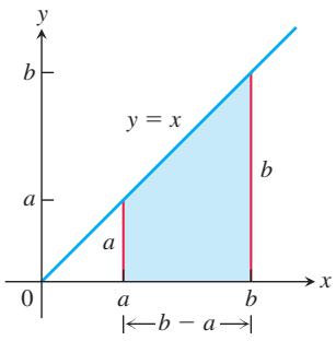
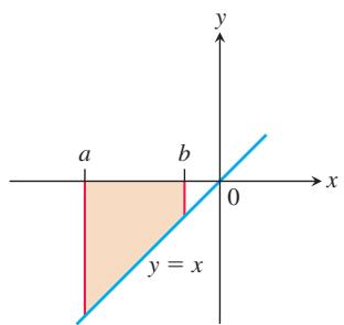
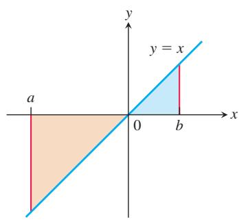
FIGURE 5.13 (a) The area of this trapezoidal region is
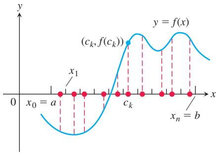
FIGURE 5.14 A sample of values of a function on an interval
Example 5 can be generalized to integrate
First write
Then, by rearranging this equation and applying Example 5, we obtain
In conclusion, we have the following rule for integrating
This computation gives the area of the trapezoid in Figure 5.13a. Equation (2) remains valid when
The following results can also be established by using a Riemann sum calculation similar to the one we used in Example 5 (Exercises 63 and 65).
Average Value of a Continuous Function Revisited
In Section 5.1 we informally introduced the average value of a nonnegative continuous function f over an interval
This formula gives us a precise definition of the average value of a continuous (or integrable) function, whether it is positive, negative, or both.
Alternatively, we can justify this formula through the following reasoning. We start with the idea from arithmetic that the average of n numbers is their sum divided by n. A continuous function f on
The average of the samples is obtained by dividing a Riemann sum for
DEFINITION If
is integrable on 𝑓 , then its average value on [ 𝑎 , 𝑏 ] , also called its mean, is [ 𝑎 , 𝑏 ] a v ( 𝑓 ) = 1 𝑏 − 𝑎 ∫ 𝑏 𝑎 𝑓 ( 𝑥 ) 𝑑 𝑥 .
EXAMPLE 6 Find the average value of
Solution From Equation (2) we see that
So the average value of f on the interval
EXAMPLE 7 Find the average value of
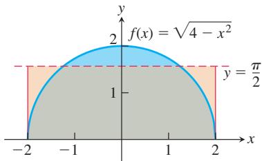
Solution We recognize
Since we know the area inside a circle, we do not need to take the limit of Riemann sums. The area between the semicircle and the x-axis from -2 to 2 can be computed using the geometry formula
FIGURE 5.15 The average value of
Because f is nonnegative, the area is also the value of the integral of f from -2 to 2,
Therefore, the average value of
Notice that the average value of f over
EXERCISES 5.3
Interpreting Limits of Sums as Integrals
Express the limits in Exercises 1–8 as definite integrals.
-
l i m | | 𝑃 | | → 0 ∑ 𝑛 𝑘 = 1 𝑐 2 𝑘 Δ 𝑥 𝑘 -
l i m | | 𝑃 | | → 0 ∑ 𝑛 𝑘 = 1 2 𝑐 3 𝑘 Δ 𝑥 𝑘 [ − 1 , 0 ] -
l i m ‖ 𝑃 ‖ → 0 ∑ 𝑛 𝑘 = 1 ( 𝑐 2 𝑘 − 3 𝑐 𝑘 ) Δ 𝑥 𝑘 𝑃 [ − 7 , 5 ] -
l i m | | 𝑃 | | → 0 ∑ 𝑛 𝑘 = 1 ( 1 𝑐 𝑘 ) Δ 𝑥 𝑘 𝑃 -
l i m | | 𝑃 | | → 0 ∑ 𝑛 𝑘 = 1 1 1 − 𝑐 𝑘 Δ 𝑥 𝑘 𝑃 -
l i m | | 𝑃 | | → 0 ∑ 𝑛 𝑘 = 1 √ 4 − 𝑐 2 𝑘 Δ 𝑥 𝑘 -
l i m | | 𝑃 | | → 0 ∑ 𝑛 𝑘 = 1 ( s e c 𝑐 𝑘 ) Δ 𝑥 𝑘 [ − 𝜋 / 4 , 0 ] -
l i m | | 𝑃 | | → 0 ∑ 𝑛 𝑘 = 1 ( t a n 𝑐 𝑘 ) Δ 𝑥 𝑘 𝑃 [ 0 , 𝜋 / 4 ]
Using the Definite Integral Rules
- Suppose that
𝑓 𝑔
Use the rules in Table 5.6 to find
a.
c.
d.
e.
- Suppose that
𝑓 ℎ
Use the rules in Table 5.6 to find
a.
b.
c.
d.
e.
- Suppose that
∫ 2 1 𝑓 ( 𝑥 ) 𝑑 𝑥 = 5
a.
c.
d.
- Suppose that
∫ 0 − 3 𝑔 ( 𝑡 ) 𝑑 𝑡 = √ 2
a.
b.
c.
d.
-
Suppose that
𝑓 ∫ 3 0 𝑓 ( 𝑧 ) 𝑑 𝑧 = 3 ∫ 4 0 𝑓 ( 𝑧 ) 𝑑 𝑧 = 7 ∫ 4 3 𝑓 ( 𝑧 ) 𝑑 𝑧 ∫ 3 4 𝑓 ( 𝑡 ) 𝑑 𝑡 -
Suppose that
ℎ ∫ 1 − 1 ℎ ( 𝑟 ) 𝑑 𝑟 = 0 ∫ 3 − 1 ℎ ( 𝑟 ) 𝑑 𝑟 = 6 ∫ 3 1 ℎ ( 𝑟 ) 𝑑 𝑟 − ∫ 1 3 ℎ ( 𝑢 ) 𝑑 𝑢
Using Known Areas to Find Integrals
In Exercises 15–22, graph the integrands and use known area formulas to evaluate the integrals.
-
∫ 4 − 2 ( 𝑥 2 + 3 ) 𝑑 𝑥 -
∫ 3 / 2 1 / 2 ( − 2 𝑥 + 4 ) 𝑑 𝑥 -
∫ 3 − 3 √ 9 − 𝑥 2 𝑑 𝑥 -
∫ 0 − 4 √ 1 6 − 𝑥 2 𝑑 𝑥 -
∫ 1 − 2 | 𝑥 | 𝑑 𝑥 -
∫ 1 − 1 ( 1 − | 𝑥 | ) 𝑑 𝑥 -
∫ 1 − 1 ( 2 − | 𝑥 | ) 𝑑 𝑥 -
∫ 1 − 1 ( 1 + √ 1 − 𝑥 2 ) 𝑑 𝑥
Use known area formulas to evaluate the integrals in Exercises 23–28.
-
∫ 𝑏 0 𝑥 2 𝑑 𝑥 , 𝑏 > 0 -
∫ 𝑏 0 4 𝑥 𝑑 𝑥 , 𝑏 > 0 -
∫ 𝑏 𝑎 2 𝑠 𝑑 𝑠 , 0 < 𝑎 < 𝑏 -
∫ 𝑏 𝑎 3 𝑡 𝑑 𝑡 , 0 < 𝑎 < 𝑏 -
𝑓 ( 𝑥 ) = √ 4 − 𝑥 2 [ − 2 , 2 ] [ 0 , 2 ] -
𝑓 ( 𝑥 ) = 3 𝑥 + √ 1 − 𝑥 2 [ − 1 , 0 ] [ − 1 , 1 ]
Evaluating Definite Integrals
Use the results of Equations (2) and (4) to evaluate the integrals in Exercises 29–40.
-
∫ √ 2 1 𝑥 𝑑 𝑥 -
∫ 2 . 5 0 . 5 𝑥 𝑑 𝑥 -
∫ 2 𝜋 𝜋 𝜃 𝑑 𝜃 -
∫ 5 √ 2 √ 2 𝑟 𝑑 𝑟 -
∫ 3 √ 7 0 𝑥 2 𝑑 𝑥 -
∫ 0 . 3 0 𝑠 2 𝑑 𝑠 -
∫ 1 / 2 0 𝑡 2 𝑑 𝑡 -
∫ 𝜋 / 2 0 𝜃 2 𝑑 𝜃 -
∫ 2 𝑎 𝑎 𝑥 𝑑 𝑥 -
∫ √ 3 𝑎 𝑥 𝑑 𝑥 -
∫ 3 √ 𝑏 0 𝑥 2 𝑑 𝑥 -
∫ 3 𝑏 0 𝑥 2 𝑑 𝑥
Use the rules in Table 5.6 and Equations (2)-(4) to evaluate the integrals in Exercises 41-50.
-
∫ 1 3 7 𝑑 𝑥 -
∫ 2 0 5 𝑥 𝑑 𝑥 -
∫ 2 0 ( 2 𝑡 − 3 ) 𝑑 𝑡 -
∫ √ 2 0 ( 𝑡 − √ 2 ) 𝑑 𝑡 -
∫ 1 2 ( 1 + 𝑧 2 ) 𝑑 𝑧 -
∫ 0 3 ( 2 𝑧 − 3 ) 𝑑 𝑧 -
∫ 2 1 3 𝑢 2 𝑑 𝑢 -
∫ 1 1 / 2 2 4 𝑢 2 𝑑 𝑢 -
∫ 2 0 ( 3 𝑥 2 + 𝑥 − 5 ) 𝑑 𝑥 -
∫ 0 1 ( 3 𝑥 2 + 𝑥 − 5 ) 𝑑 𝑥
Finding Area by Definite Integrals
In Exercises 51–54, use a definite integral to find the area of the region between the given curve and the x-axis on the interval
-
𝑦 = 3 𝑥 2 -
𝑦 = 𝜋 𝑥 2 -
𝑦 = 2 𝑥 -
𝑦 = 𝑥 2 + 1
Finding Average Value
In Exercises 55–62, graph the function and find its average value over the given interval.
-
𝑓 ( 𝑥 ) = 𝑥 2 − 1 [ 0 , √ 3 ] -
𝑓 ( 𝑥 ) = − 𝑥 2 2 [ 0 , 3 ] -
𝑓 ( 𝑥 ) = − 3 𝑥 2 − 1 -
𝑓 ( 𝑥 ) = 3 𝑥 2 − 3 -
𝑓 ( 𝑡 ) = ( 𝑡 − 1 ) 2 -
𝑓 ( 𝑡 ) = 𝑡 2 − 𝑡 [ − 2 , 1 ] -
𝑔 ( 𝑥 ) = | 𝑥 | − 1 [ − 1 , 1 ] [ 1 , 3 ] [ − 1 , 3 ] -
ℎ ( 𝑥 ) = − | 𝑥 | [ − 1 , 0 ] [ 0 , 1 ] [ − 1 , 1 ]
Definite Integrals as Limits of Sums
Use the method of Example 5a or Equation (1) to evaluate the definite integrals in Exercises 63–70.
-
∫ 𝑏 𝑎 𝑐 𝑑 𝑥 -
∫ 2 0 ( 2 𝑥 + 1 ) 𝑑 𝑥 -
∫ 𝑏 𝑎 𝑥 2 𝑑 𝑥 , 𝑎 < 𝑏 -
∫ 0 − 1 ( 𝑥 − 𝑥 2 ) 𝑑 𝑥 -
∫ 2 − 1 ( 3 𝑥 2 − 2 𝑥 + 1 ) 𝑑 𝑥 -
∫ 1 − 1 𝑥 3 𝑑 𝑥 -
∫ 𝑏 𝑎 𝑥 3 𝑑 𝑥 , 𝑎 < 𝑏 -
∫ 1 0 ( 3 𝑥 − 𝑥 3 ) 𝑑 𝑥
Theory and Examples
- What values of a and b, with a < b, maximize the value of
(Hint: Where is the integrand positive?)
- What values of a and b, with a < b, minimize the value of
Add these to arrive at an improved estimate of
-
Show that the value of
∫ 1 0 s i n ( 𝑥 2 ) 𝑑 𝑥 -
Show that the value of
∫ 1 0 √ 𝑥 + 8 𝑑 𝑥 2 √ 2 ≈ 2 . 8 -
Integrals of nonnegative functions Use the Max-Min Inequality to show that if
𝑓
-
Use the inequality
s i n 𝑥 ≤ 𝑥 𝑥 ≥ 0 ∫ 1 0 s i n 𝑥 𝑑 𝑥 -
The inequality
s e c 𝑥 ≥ 1 + ( 𝑥 2 / 2 ) ( − 𝜋 / 2 , 𝜋 / 2 ) ∫ 1 0 s e c 𝑥 𝑑 𝑥 -
If
a v ( 𝑓 ) 𝑓 ( 𝑥 ) [ 𝑎 , 𝑏 ] a v ( 𝑓 ) [ 𝑎 , 𝑏 ]
Give reasons for your answer.
- It would be nice if average values of integrable functions obeyed the following rules on an interval
[ 𝑎 , 𝑏 ]
a.
b.
Do these rules ever hold? Give reasons for your answers.
- Upper and lower sums for increasing functions
a. Suppose the graph of a continuous function
b. Suppose that instead of being equal, the lengths
where
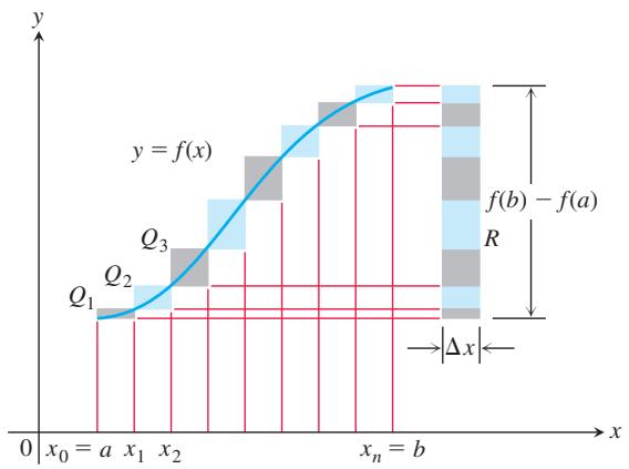
- Upper and lower sums for decreasing functions (Continuation of Exercise 83.)
a. Draw a figure like the one in Exercise 83 for a continuous function
b. Suppose that instead of being equal, the lengths
of Exercise 83b still holds and hence
- Use the formula
to find the area under the curve
a. Partition the interval
b. Find the limit of U as
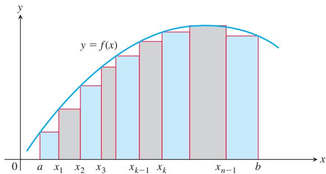
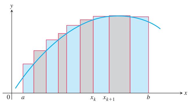
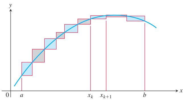
- Suppose that
𝑓 [ 𝑎 , 𝑏 ]
as shown, divide
a. If
and the shaded regions in the first part of the figure.
b. If
and the shaded regions in the second part of the figure.
c. Explain the connection between

-
We say
𝑓 [ 𝑎 , 𝑏 ] 𝜀 > 0 𝛿 > 0 𝑥 1 , 𝑥 2 [ 𝑎 , 𝑏 ] | 𝑥 1 − 𝑥 2 | < 𝛿 | 𝑓 ( 𝑥 1 ) − 𝑓 ( 𝑥 2 ) | < 𝜀 [ 𝑎 , 𝑏 ] 𝑓 𝜀 > 0 𝑈 − 𝐿 ≤ 𝜀 ⋅ ( 𝑏 − 𝑎 ) Δ 𝑥 𝑘 -
If you average 48 km/h on a 240-km trip and then return over the same 240 km at the rate of 80 km/h, what is your average speed for the trip? Give reasons for your answer.
-
Integrals of functions that are equal except at one point Suppose that
𝑓 ( 𝑥 ) [ 𝑎 , 𝑏 ] 𝑔 ( 𝑥 ) [ 𝑎 , 𝑏 ] 𝑔 ( 𝑥 ) = 𝑓 ( 𝑥 ) 𝑐 ∈ [ 𝑎 , 𝑏 ] 𝑔 ( 𝑥 ) [ 𝑎 , 𝑏 ] ∫ 𝑏 𝑎 𝑔 ( 𝑥 ) 𝑑 𝑥 = ∫ 𝑏 𝑎 𝑓 ( 𝑥 ) 𝑑 𝑥 𝑛 -
Some integrable functions that are not continuous
a. The floor function
b. The function
COMPUTER EXPLORATIONS
If your CAS can draw rectangles associated with Riemann sums, use it to draw rectangles associated with Riemann sums that converge to the integrals in Exercises 91–96. Use n = 4, 10, 20, and 50 subintervals of equal length in each case.
-
∫ 1 0 ( 1 − 𝑥 ) 𝑑 𝑥 = 1 2 -
∫ 1 0 ( 𝑥 2 + 1 ) 𝑑 𝑥 = 4 3
-
∫ 1 − 1 | 𝑥 | 𝑑 𝑥 = 1 -
∫ 2 1 1 𝑥 𝑑 𝑥
In Exercises 97–104, use a CAS to perform the following steps:
a. Plot the functions over the given interval.
b. Partition the interval into n = 100, 200, and 1000 sub-intervals of equal length, and evaluate the function at the midpoint of each subinterval.
c. Compute the average value of the function values generated in part (b).
d. Solve the equation
-
𝑓 ( 𝑥 ) = 𝑥 s i n 1 𝑥 [ 𝜋 4 , 𝜋 ] -
𝑓 ( 𝑥 ) = 𝑥 s i n 2 1 𝑥 [ 𝜋 4 , 𝜋 ] -
𝑓 ( 𝑥 ) = 𝑥 𝑒 − 𝑥 -
𝑓 ( 𝑥 ) = 𝑒 − 𝑥 2 -
𝑓 ( 𝑥 ) = l n 𝑥 𝑥
on [2,5]
𝑓 ( 𝑥 ) = 1 √ 1 − 𝑥 2 [ 0 , 1 2 ]
5.4 The Fundamental Theorem of Calculus
HISTORICAL BIOGRAPHY
Sir Isaac Newton
(1642-1727)
In his youth in England, Newton was interested in mechanical devices and their underlying theories. He even constructed lanterns and windmills that he designed. During the 1670s and 1680s, he built his reputation as a scientific genius. His contributions included the theory of universal gravitation, the laws of motion, methods of calculus, and the composition of white light. To know more, visit the companion Website.
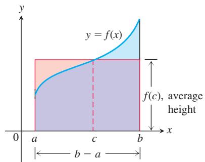
FIGURE 5.16 The value
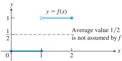
FIGURE 5.17 A discontinuous function need not assume its average value.
In this section we present the Fundamental Theorem of Calculus, which is the central theorem of integral calculus. It connects integration and differentiation, enabling us to compute integrals by using an antiderivative of the integrand function, rather than by taking limits of Riemann sums as we did in Section 5.3. Leibniz and Newton exploited this relationship and started mathematical developments that fueled the scientific revolution for the next 200 years.
Along the way, we will present an integral version of the Mean Value Theorem, which is another important theorem of integral calculus and is used to prove the Fundamental Theorem. We also find that the net change of a function over an interval is the integral of its rate of change, as suggested by Example 2 in Section 5.1.
Mean Value Theorem for Definite Integrals
In the previous section we defined the average value of a continuous function over a closed interval
The graph in Figure 5.16 shows a positive continuous function
THEOREM 3—The Mean Value Theorem for Definite Integrals
If f is continuous on
Proof If we divide all three expressions in the Max-Min Inequality (Table 5.6, Rule 6) by
Since
The continuity of
EXAMPLE 1 Show that if
then
Solution The average value of f on
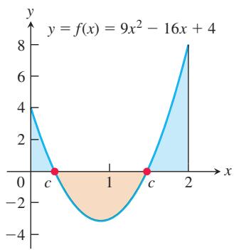
FIGURE 5.18 The function
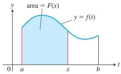
FIGURE 5.19 The function
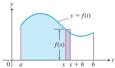
FIGURE 5.20 In Equation (1),
By the Mean Value Theorem for Definite Integrals,
Fundamental Theorem, Part 1
It can be very difficult to compute definite integrals by taking the limit of Riemann sums. We now develop a powerful new method for evaluating definite integrals, based on using antiderivatives. This method combines the two strands of calculus. One strand involves the idea of taking the limits of finite sums to obtain a definite integral, and the other strand contains derivatives and antiderivatives. They come together in the Fundamental Theorem of Calculus. We begin by considering how to differentiate a certain type of function that is described as an integral.
If
For example, if f is nonnegative and x lies to the right of a, then
Equation (1) gives a useful way to define new functions (as we will see in Section 7.1), but its key importance is the connection that it makes between integrals and derivatives. If f is a continuous function, then the Fundamental Theorem asserts that F is a differentiable function of x whose derivative is f itself. That is, at each x in the interval
To gain some insight into why this holds, we look at the geometry behind it.
If
If h > 0, then
Dividing both sides by h, we see that the value of the difference quotient is very close to the value of
This approximation improves as h approaches 0. It is reasonable to expect that
This equation is true even if the function
THEOREM 4—The Fundamental Theorem of Calculus, Part 1
If f is continuous on
Before proving Theorem 4, we look at several examples to gain an understanding of what it says. In each of these examples, notice that the independent variable x appears in either the upper or the lower limit of integration (either as part of a formula or by itself). The independent variable on which y depends in these examples is x, while t is merely a dummy variable in the integral.
EXAMPLE 2 Use the Fundamental Theorem to find dy/dx if
Solution We calculate the derivatives with respect to the independent variable x.
(c) The upper limit of integration is not
We must therefore apply the Chain Rule to find dy/dx:
Proof of Theorem 4 We prove the Fundamental Theorem, Part 1, by applying the definition of the derivative directly to the function
and showing that its limit as
According to the Mean Value Theorem for Definite Integrals, there is some point c between x and
As
Hence we have shown that, for any x in
and therefore F is differentiable at x. Since differentiability implies continuity, this also shows that F is continuous on the open interval
Fundamental Theorem, Part 2 (The Evaluation Theorem)
We now come to the second part of the Fundamental Theorem of Calculus. This part describes how to evaluate definite integrals without having to calculate limits of Riemann sums. Instead we find and evaluate an antiderivative at the upper and lower limits of integration.
THEOREM 4 (Continued)—The Fundamental Theorem of Calculus, Part 2
If f is continuous over
Proof Part 1 of the Fundamental Theorem tells us that an antiderivative of
Thus, if
Evaluating
The Evaluation Theorem is important because it says that to calculate the definite integral of
-
Find an antiderivative F of f, and
-
Calculate the number
𝐹 ( 𝑏 ) − 𝐹 ( 𝑎 ) ∫ 𝑏 𝑎 𝑓 ( 𝑥 ) 𝑑 𝑥
This process is much easier than computing Riemann sums and finding their limit. The power of the theorem follows from the realization that the definite integral, which is defined by a complicated process involving all of the values of the function f over
depending on whether F has one or more terms.
EXAMPLE 3 We calculate several definite integrals using the Evaluation Theorem, rather than by taking limits of Riemann sums.
Exercise 82 offers another proof of the Evaluation Theorem, bringing together the ideas of Riemann sums, the Mean Value Theorem, and the definition of the definite integral.
The Integral of a Rate
We can interpret Part 2 of the Fundamental Theorem in another way. If F is any antiderivative of f, then
Now
THEOREM 5—The Net Change Theorem
The net change in a differentiable function
EXAMPLE 4 Here are several interpretations of the Net Change Theorem.
(a) If
which is the cost of increasing production from
(b) If an object with position function
so the integral of velocity is the displacement over the time interval
If we rearrange Equation (6) as
we see that the Net Change Theorem also says that the final value of a function
EXAMPLE 5 Consider again our analysis of a heavy rock blown straight up from the ground by a dynamite blast (Example 2, Section 5.1). The velocity of the rock at any time t during its motion was given as
(a) Find the displacement of the rock during the time period
(b) Find the total distance traveled during this time period.
Solution
(a) From Example 4b, the displacement is the integral
This means that the height of the rock is 78.4 m above the ground 8 s after the explosion, which agrees with our conclusion in Example 2, Section 5.1.
(b) As we noted in Table 5.3, the velocity function
Again, this calculation agrees with our conclusion in Example 2, Section 5.1. That is, the total distance of 166.6 m traveled by the rock during the time period
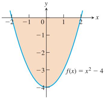
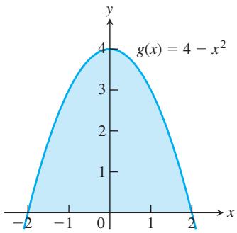
FIGURE 5.21 These graphs enclose the same amount of area with the x-axis, but the definite integrals of the two functions over
The Relationship Between Integration and Differentiation
The conclusions of the Fundamental Theorem tell us several things. Equation (2) can be rewritten as
which says that if you first integrate the function f and then differentiate the result, you get the function f back again. Likewise, replacing b by x and x by t in Equation (6) gives
so that if you first differentiate the function F and then integrate the result, you get the function F back (adjusted by an integration constant). In a sense, the processes of integration and differentiation are “inverses” of each other. The Fundamental Theorem also says that every continuous function f has an antiderivative F. It shows the importance of finding antiderivatives in order to evaluate definite integrals easily. Furthermore, it says that the differential equation
Total Area
Area is always a nonnegative quantity. The Riemann sum approximations contain terms such as
EXAMPLE 6 Figure 5.21 shows the graph of
(a) the definite integral over the interval
(b) the area between the graph and the x-axis over
Solution
and
(b) In both cases, the area between the curve and the x-axis over
To compute the area of the region bounded by the graph of a function
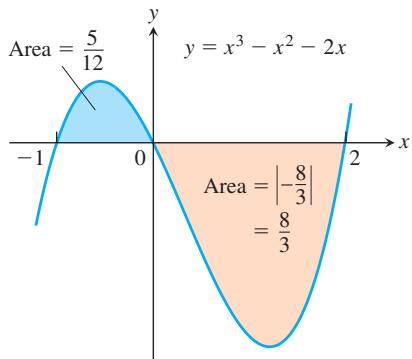
FIGURE 5.22 The total area between
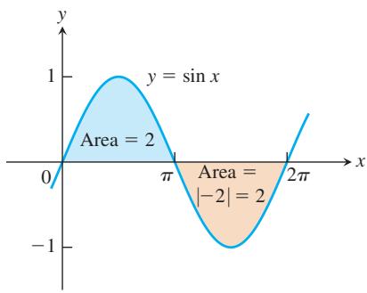
FIGURE 5.23 The region between the curve
EXAMPLE 7 Figure 5.22 shows the graph of the function
(a) the definite integral of
(b) the area between the graph of
Solution
(a) The definite integral for
The definite integral is zero because the portions of the graph above and below the x-axis make canceling contributions.
(b) The area between the graph of
The second integral gives a negative value. The area between the graph and the axis is obtained by adding the absolute values,
Summary:
To find the area between the graph of
-
Subdivide
[ 𝑎 , 𝑏 ] -
Integrate f over each subinterval.
-
Add the absolute values of the integrals.
EXAMPLE 8 Find the area of the region between the x-axis and the graph of
Solution First find the zeros of
the zeros are x = 0, -1, and 2 (Figure 5.23). The zeros subdivide
The total enclosed area is obtained by adding the absolute values of the calculated integrals.
EXERCISES 5.4
Evaluating Integrals
Evaluate the integrals in Exercises 1–34.
-
∫ 2 0 𝑥 ( 𝑥 − 3 ) 𝑑 𝑥 -
∫ 1 − 1 ( 𝑥 2 − 2 𝑥 + 3 ) 𝑑 𝑥 -
∫ 2 − 2 ( 𝑥 + 3 ) 2 𝑑 𝑥 -
∫ 1 − 1 𝑥 2 9 9 𝑑 𝑥 -
∫ 4 1 ( 3 𝑥 2 − 𝑥 3 4 ) 𝑑 𝑥 -
∫ 3 − 2 ( 𝑥 3 − 2 𝑥 + 3 ) 𝑑 𝑥 -
∫ 1 0 ( 𝑥 2 + √ 𝑥 ) 𝑑 𝑥 -
∫ 3 2 1 𝑥 − 6 / 5 𝑑 𝑥 -
∫ 𝜋 / 3 0 2 s e c 2 𝑥 𝑑 𝑥 -
∫ 𝜋 0 ( 1 + c o s 𝑥 ) 𝑑 𝑥 -
∫ 3 𝜋 / 4 𝜋 / 4 c s c 𝜃 c o t 𝜃 𝑑 𝜃 -
∫ 𝜋 / 3 0 4 s i n 𝑢 c o s 2 𝑢 𝑑 𝑢 -
∫ 0 𝜋 / 2 1 + c o s 2 𝑡 2 𝑑 𝑡 -
∫ 𝜋 / 3 − 𝜋 / 3 s i n 2 𝑡 𝑑 𝑡 -
∫ 𝜋 / 4 0 t a n 2 𝑥 𝑑 𝑥 -
∫ 𝜋 / 6 0 ( s e c 𝑥 + t a n 𝑥 ) 2 𝑑 𝑥 -
∫ 𝜋 / 8 0 s i n 2 𝑥 𝑑 𝑥 -
∫ − 𝜋 / 4 − 𝜋 / 3 ( 4 s e c 2 𝑡 + 𝜋 𝑡 2 ) 𝑑 𝑡 -
∫ − 1 1 ( 𝑟 + 1 ) 2 𝑑 𝑟 -
∫ √ 3 − √ 3 ( 𝑡 + 1 ) ( 𝑡 2 + 4 ) 𝑑 𝑡 -
∫ 1 √ 2 ( 𝑢 7 2 − 1 𝑢 5 ) 𝑑 𝑢 -
∫ − 1 − 3 𝑦 5 − 2 𝑦 𝑦 3 𝑑 𝑦 -
∫ √ 2 1 𝑠 2 + √ 𝑠 𝑠 2 𝑑 𝑠 -
∫ 8 1 ( 𝑥 1 / 3 + 1 ) ( 2 − 𝑥 2 / 3 ) 𝑥 1 / 3 𝑑 𝑥 -
∫ 𝜋 / 2 𝜋 / 6 s i n 2 𝑥 2 s i n 𝑥 𝑑 𝑥 -
∫ 𝜋 / 3 0 ( c o s 𝑥 + s e c 𝑥 ) 2 𝑑 𝑥 -
∫ 4 − 4 | 𝑥 | 𝑑 𝑥 -
∫ 𝜋 0 1 2 ( c o s 𝑥 + | c o s 𝑥 | ) 𝑑 𝑥 -
∫ l n 2 0 𝑒 3 𝑥 𝑑 𝑥 -
∫ 2 1 ( 1 𝑥 − 𝑒 − 𝑥 ) 𝑑 𝑥 -
∫ 1 / 2 0 4 √ 1 − 𝑥 2 𝑑 𝑥 -
∫ 1 / √ 3 0 𝑑 𝑥 1 + 4 𝑥 2 -
∫ 4 2 𝑥 𝜋 − 1 𝑑 𝑥 -
∫ 0 − 1 𝜋 𝑥 − 1 𝑑 𝑥
In Exercises 35–38, guess an antiderivative for the integrand function. Validate your guess by differentiation, and then evaluate the given definite integral. (Hint: Keep the Chain Rule in mind when trying to guess an antiderivative. You will learn how to find such antiderivatives in the next section.)
-
∫ 1 0 𝑥 𝑒 𝑥 2 𝑑 𝑥 -
∫ 2 1 l n 𝑥 𝑥 𝑑 𝑥 -
∫ 5 2 𝑥 𝑑 𝑥 √ 1 + 𝑥 2 -
∫ 𝜋 / 3 0 s i n 2 𝑥 c o s 𝑥 𝑑 𝑥
Derivatives of Integrals
Find the derivatives in Exercises 39–44.
a. by evaluating the integral and differentiating the result.
b. by differentiating the integral directly.
39.
-
𝑑 𝑑 𝑥 ∫ s i n 𝑥 1 3 𝑡 2 𝑑 𝑡 -
𝑑 𝑑 𝑡 ∫ 𝑡 4 0 √ 𝑢 𝑑 𝑢 -
𝑑 𝑑 𝜃 ∫ t a n 𝜃 0 s e c 2 𝑦 𝑑 𝑦 -
𝑑 𝑑 𝑥 ∫ 𝑥 3 0 𝑒 − 𝑡 𝑑 𝑡 -
𝑑 𝑑 𝑡 ∫ √ 𝑡 0 ( 𝑥 4 + 3 √ 1 − 𝑥 2 ) 𝑑 𝑥
Find
-
𝑦 = ∫ 𝑥 0 √ 1 + 𝑡 2 𝑑 𝑡 -
𝑦 = ∫ 𝑥 1 1 𝑡 𝑑 𝑡 , 𝑥 > 0 -
𝑦 = ∫ 0 √ 𝑥 s i n 𝑡 2 𝑑 𝑡 -
𝑦 = 𝑥 ∫ 𝑥 2 2 s i n 𝑡 3 𝑑 𝑡 -
𝑦 = ∫ 𝑥 − 1 𝑡 2 𝑡 2 + 4 𝑑 𝑡 − ∫ 𝑥 3 𝑡 2 𝑡 2 + 4 𝑑 𝑡 -
𝑦 = ( ∫ 𝑥 0 ( 𝑡 3 + 1 ) 1 0 𝑑 𝑡 ) 3 -
𝑦 = ∫ s i n 𝑥 0 𝑑 𝑡 √ 1 − 𝑡 2 , | 𝑥 | < 𝜋 2 -
𝑦 = ∫ 0 t a n 𝑥 𝑑 𝑡 1 + 𝑡 2 -
𝑦 = ∫ 𝑒 𝑥 2 0 1 √ 𝑡 𝑑 𝑡 -
𝑦 = ∫ 1 2 𝑥 3 √ 𝑡 𝑑 𝑡 -
𝑦 = ∫ a r c s i n 𝑥 0 c o s 𝑡 𝑑 𝑡 -
𝑦 = ∫ 𝑥 1 / 𝜋 − 1 a r c s i n 𝑡 𝑑 𝑡
Area
In Exercises 57–60, find the total area between the region and the x-axis.
-
𝑦 = − 𝑥 2 − 2 𝑥 , − 3 ≤ 𝑥 ≤ 2 -
𝑦 = 3 𝑥 2 − 3 , − 2 ≤ 𝑥 ≤ 2 -
𝑦 = 𝑥 3 − 3 𝑥 2 + 2 𝑥 , 0 ≤ 𝑥 ≤ 2 -
𝑦 = 𝑥 1 / 3 − 𝑥 , − 1 ≤ 𝑥 ≤ 8
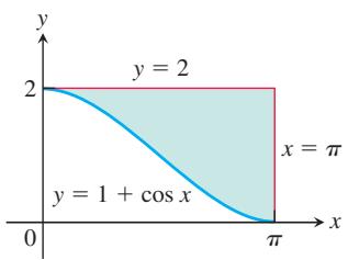
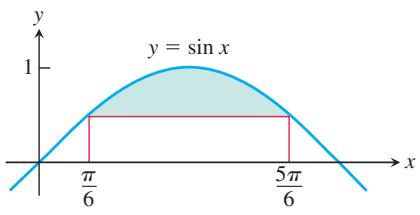
Find the areas of the shaded regions in Exercises 61–64.
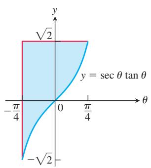
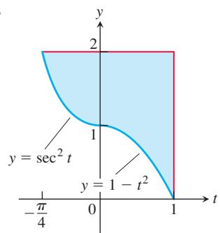
Initial Value Problems
Each of the following functions solves one of the initial value problems in Exercises 65–68. Which function solves which problem? Give brief reasons for your answers.
𝑑 𝑦 𝑑 𝑥 = 1 𝑥 , 𝑦 ( 𝜋 ) = − 3
Express the solutions of the initial value problems in Exercises 69 and 70 in terms of integrals.
-
𝑑 𝑦 𝑑 𝑥 = s e c 𝑥 , 𝑦 ( 2 ) = 3 -
𝑑 𝑦 𝑑 𝑥 = √ 1 + 𝑥 2 , 𝑦 ( 1 ) = − 2
For Exercises 71 and 72, find a function f satisfying each equation.
Theory and Examples
-
Archimedes’ area formula for parabolic arches Archimedes (287–212 B.C.), inventor, military engineer, physicist, and the greatest mathematician of classical times in the Western world, discovered that the area under a parabolic arch is two-thirds the base times the height. Sketch the parabolic arch
𝑦 = ℎ − ( 4 ℎ / 𝑏 2 ) 𝑥 2 − 𝑏 / 2 ≤ 𝑥 ≤ 𝑏 / 2 -
Show that if k is a positive constant, then the area between the x-axis and one arch of the curve
𝑦 = s i n 𝑘 𝑥 -
Cost from marginal cost The marginal cost of printing a poster when x posters have been printed is
dollars. Find
In Exercises 76–78, guess an antiderivative and validate your guess by differentiation. (Hint: Keep the Chain Rule in mind when trying to guess an antiderivative. You will learn how to find such antiderivatives in the next section.)
- Revenue from marginal revenue Suppose that a company’s marginal revenue from the manufacture and sale of eggbeaters is
where r is measured in thousands of dollars and x in thousands of units. How much money should the company expect from a production run of x = 3 thousand eggbeaters? To find out, integrate the marginal revenue from x = 0 to x = 3.
- The temperature
𝑇 ( ∘ C )
a. Find the room’s temperature when
b. Find the room’s average temperature for
- The height
𝐻 ( m ) 𝑡
a. Find the tree’s height when
b. Find the tree’s average height for
-
Suppose that
∫ 𝑥 1 𝑓 ( 𝑡 ) 𝑑 𝑡 = 𝑥 2 − 2 𝑥 + 1 𝑓 ( 𝑥 ) -
Find
𝑓 ( 4 ) ∫ 𝑥 0 𝑓 ( 𝑡 ) 𝑑 𝑡 = 𝑥 c o s 𝜋 𝑥 -
Find the linearization of
at x = -1.
- Suppose that
𝑓 𝑥 𝑓 ( 1 ) = 0
Give reasons for your answers.
a. g is a differentiable function of x.
b. g is a continuous function of x.
c. The graph of
d. g has a local maximum at x = 1.
e. g has a local minimum at x = 1.
f. The graph of g has an inflection point at x = 1.
g. The graph of
- Another proof of the Evaluation Theorem
a. Let
b. Apply the Mean Value Theorem to each term to show that
c. From part (b) and the definition of the definite integral, show that
meters. Use the graph to answer the following questions. Give reasons for your answers.
a. What is the particle’s velocity at time
b. Is the acceleration of the particle at time
c. What is the particle’s position at time
d. At what time during the first 9 seconds does s have its largest value?
e. Approximately when is the acceleration zero?
f. When is the particle moving toward the origin? Away from the origin?
g. On which side of the origin does the particle lie at time t = 9?
- Find
l i m 𝑥 → ∞ 1 √ 𝑥 ∫ 𝑥 1 𝑑 𝑡 √ 𝑡 .
COMPUTER EXPLORATIONS
In Exercises 87–90, let
a. Plot the functions f and F together over
b. Solve the equation
c. Over what intervals (approximately) is the function
d. Calculate the derivative
𝑓 ( 𝑥 ) = 𝑥 3 − 4 𝑥 2 + 3 𝑥 , [ 0 , 4 ]
In Exercises 91–94, let
a. Find the domain of
b. Calculate
c. Calculate
d. Using the information from parts (a)-(c), draw a rough handsketch of
-
𝑎 = 1 , 𝑢 ( 𝑥 ) = 𝑥 2 , 𝑓 ( 𝑥 ) = √ 1 − 𝑥 2 -
𝑎 = 0 , 𝑢 ( 𝑥 ) = 𝑥 2 , 𝑓 ( 𝑥 ) = √ 1 − 𝑥 2 -
𝑎 = 0 , 𝑢 ( 𝑥 ) = 1 − 𝑥 , 𝑓 ( 𝑥 ) = 𝑥 2 − 2 𝑥 − 3 -
𝑎 = 0 , 𝑢 ( 𝑥 ) = 1 − 𝑥 2 , 𝑓 ( 𝑥 ) = 𝑥 2 − 2 𝑥 − 3
In Exercises 95 and 96, assume that
-
Calculate
𝑑 𝑑 𝑥 ∫ 𝑢 ( 𝑥 ) 𝑎 𝑓 ( 𝑡 ) 𝑑 𝑡 -
Calculate
𝑑 2 𝑑 𝑥 2 ∫ 𝑢 ( 𝑥 ) 𝑎 𝑓 ( 𝑡 ) 𝑑 𝑡
5.5 Indefinite Integrals and the Substitution Method
The Fundamental Theorem of Calculus says that a definite integral of a continuous function can be computed directly if we can find an antiderivative of the function. In Section 4.8 we defined the indefinite integral of the function
where C is any arbitrary constant. The connection between antiderivatives and the definite integral stated in the Fundamental Theorem now explains this notation:
When finding the indefinite integral of a function f, remember that it always includes an arbitrary constant C.
We must keep in mind the difference between definite and indefinite integrals. A definite integral
So far, we have only been able to find antiderivatives of functions that are clearly recognizable as derivatives. In this section we begin to develop more general techniques for finding antiderivatives of functions.
Substitution: Running the Chain Rule Backwards
If
From another point of view, this same equation says that
The integral in Equation (1) is equal to the simpler integral
which suggests that we can substitute the simpler expression du for
EXAMPLE 1 Find the integral
Solution We set
so that by substitution we have
Solution The integral does not fit the formula
with
which is not precisely dx. The constant factor 2 is missing from the integral. However, we can introduce this factor after the integral sign if we compensate for it by introducing a factor of 1/2 in front of the integral sign. So we write
The substitutions in Examples 1 and 2 are instances of the following general rule.
THEOREM 6—The Substitution Rule
If
Proof By the Chain Rule,
If we make the substitution
The use of the variable u in the Substitution Rule is traditional (sometimes it is referred to as u-substitution), but any letter can be used, such as v, t,
The Substitution Method to evaluate
-
Substitute
𝑢 = 𝑔 ( 𝑥 ) 𝑑 𝑢 = ( 𝑑 𝑢 / 𝑑 𝑥 ) 𝑑 𝑥 = 𝑔 ′ ( 𝑥 ) 𝑑 𝑥 ∫ 𝑓 ( 𝑢 ) 𝑑 𝑢 -
Integrate with respect to u.
-
Replace u by
𝑔 ( 𝑥 )
EXAMPLE 3 Find
Solution We substitute
EXAMPLE 4 Find
Solution We let
There is another approach to this problem. With
HISTORICAL BIOGRAPHY
Birkhoff attended Harvard and the University of Chicago. He received his PhD from Chicago in 1907 for his dissertation on differential equations. He also worked on the four-color problem (colors required to produce a map) and applying mathematics to aesthetics in art, poetry, and music.
To know more, visit the companion Website.
We can verify this solution by differentiating and checking that we obtain the original function
EXAMPLE 5 Sometimes we observe that a power of x appears in the integrand that is one less than the power of x appearing in the argument of a function we want to integrate. This observation immediately suggests we try a substitution for the higher power of x. For example, in the integral below we see that
It may happen that an extra factor of x appears in the integrand when we try a substitution
Solution Our previous experience with the integral in Example 2 suggests the substitution
However, in this example the integrand contains an extra factor of x that multiplies the factor
The integration now becomes
EXAMPLE 7 Sometimes we can use trigonometric identities to transform an integral we do not know how to evaluate into one that we can evaluate using the Substitution Rule.
EXAMPLE 8 An integrand may require some algebraic manipulation before the substitution method can be applied. This example gives two integrals for which we simplify by multiplying the integrand by an algebraic form equal to 1 before attempting a substitution.
The integrals of
Integrals of the tangent, cotangent, secant, and cosecant functions
Trying Different Substitutions
The success of the substitution method depends on finding a substitution that changes an integral we cannot directly evaluate into one that we can. Finding the right substitution gets easier with practice and experience. If your first substitution fails, try another substitution, possibly coupled with other algebraic or trigonometric simplifications to the integrand. Several more complicated types of substitutions will be studied in Chapter 8.
Solution We use the substitution method of integration as an exploratory tool. First we substitute for the most troublesome part of the integrand and see how things work out. For the integral here, we might try
Method 1: Substitute
Method 2: Substitute
EXERCISES 5.5
Evaluating Indefinite Integrals
In Exercises 1–16, make the given substitutions to evaluate the indefinite integrals.
-
∫ 2 ( 2 𝑥 + 4 ) 5 𝑑 𝑥 , 𝑢 = 2 𝑥 + 4 -
∫ 7 √ 7 𝑥 − 1 𝑑 𝑥 , 𝑢 = 7 𝑥 − 1 -
∫ 2 𝑥 ( 𝑥 2 + 5 ) − 4 𝑑 𝑥 , 𝑢 = 𝑥 2 + 5 -
∫ 4 𝑥 3 ( 𝑥 4 + 1 ) 2 𝑑 𝑥 , 𝑢 = 𝑥 4 + 1 -
∫ ( 3 𝑥 + 2 ) ( 3 𝑥 2 + 4 𝑥 ) 4 𝑑 𝑥 , 𝑢 = 3 𝑥 2 + 4 𝑥 -
∫ ( 1 + √ 𝑥 ) 1 / 3 √ 𝑥 𝑑 𝑥 , 𝑢 = 1 + √ 𝑥
-
∫ s i n 3 𝑥 𝑑 𝑥 , 𝑢 = 3 𝑥 -
∫ 𝑥 s i n ( 2 𝑥 2 ) 𝑑 𝑥 , 𝑢 = 2 𝑥 2 -
∫ s e c 2 𝑡 t a n 2 𝑡 𝑑 𝑡 , 𝑢 = 2 𝑡 -
∫ ( 1 − c o s 𝑡 2 ) 2 s i n 𝑡 2 𝑑 𝑡 , 𝑢 = 1 − c o s 𝑡 2 -
∫ 9 𝑟 2 𝑑 𝑟 √ 1 − 𝑟 3 , 𝑢 = 1 − 𝑟 3 -
∫ 1 2 ( 𝑦 4 + 4 𝑦 2 + 1 ) 2 ( 𝑦 3 + 2 𝑦 ) 𝑑 𝑦 , 𝑢 = 𝑦 4 + 4 𝑦 2 + 1 -
∫ √ 𝑥 s i n 2 ( 𝑥 3 / 2 − 1 ) 𝑑 𝑥 , 𝑢 = 𝑥 3 / 2 − 1 -
∫ 1 𝑥 2 c o s 2 ( 1 𝑥 ) 𝑑 𝑥 , 𝑢 = 1 𝑥 -
∫ c s c 2 2 𝜃 c o t 2 𝜃 𝑑 𝜃 𝑢 = c o t 2 𝜃 𝑢 = c s c 2 𝜃 -
∫ 𝑑 𝑥 √ 5 𝑥 + 8 𝑢 = 5 𝑥 + 8 𝑢 = √ 5 𝑥 + 8
Evaluate the integrals in Exercises 17–66.
-
∫ √ 3 − 2 𝑠 𝑑 𝑠 -
∫ 1 √ 5 𝑠 + 4 𝑑 𝑠 -
∫ 𝜃 4 √ 1 − 𝜃 2 𝑑 𝜃 -
∫ 3 𝑦 √ 7 − 3 𝑦 2 𝑑 𝑦 -
∫ 1 √ 𝑥 ( 1 + √ 𝑥 ) 2 𝑑 𝑥 -
∫ √ s i n 𝑥 c o s 3 𝑥 𝑑 𝑥 -
∫ s e c 2 ( 3 𝑥 + 2 ) 𝑑 𝑥 -
∫ t a n 2 𝑥 s e c 2 𝑥 𝑑 𝑥 -
∫ s i n 5 𝑥 3 c o s 𝑥 3 𝑑 𝑥 -
∫ t a n 7 𝑥 2 s e c 2 𝑥 2 𝑑 𝑥 -
∫ 𝑟 2 ( 𝑟 3 1 8 − 1 ) 5 𝑑 𝑟 -
∫ 𝑟 4 ( 7 − 𝑟 5 1 0 ) 3 𝑑 𝑟 -
∫ 𝑥 1 / 2 s i n ( 𝑥 3 / 2 + 1 ) 𝑑 𝑥 -
∫ c s c ( 𝑣 − 𝜋 2 ) c o t ( 𝑣 − 𝜋 2 ) 𝑑 𝜈 -
∫ s i n ( 2 𝑡 + 1 ) c o s 2 ( 2 𝑡 + 1 ) 𝑑 𝑡 -
∫ s e c 𝑧 t a n 𝑧 √ s e c 𝑧 𝑑 𝑧 -
∫ 1 √ 𝑡 c o s ( √ 𝑡 + 3 ) 𝑑 𝑡 -
∫ 1 𝜃 2 s i n 1 𝜃 c o s 1 𝜃 𝑑 𝜃 -
∫ c o s √ 𝜃 √ 𝜃 s i n 2 √ 𝜃 𝑑 𝜃 -
∫ 𝑥 √ 1 + 𝑥 𝑑 𝑥 -
∫ √ 𝑥 − 1 𝑥 5 𝑑 𝑥 -
∫ 1 𝑥 2 √ 2 − 1 𝑥 𝑑 𝑥 -
∫ 1 𝑥 3 √ 𝑥 2 − 1 𝑥 2 𝑑 𝑥 -
∫ √ 𝑥 3 − 3 𝑥 1 1 𝑑 𝑥 -
∫ √ 𝑥 4 𝑥 3 − 1 𝑑 𝑥 -
∫ 𝑥 ( 𝑥 − 1 ) 1 0 𝑑 𝑥 -
∫ 𝑥 √ 4 − 𝑥 𝑑 𝑥 -
∫ ( 𝑥 + 1 ) 2 ( 1 − 𝑥 ) 5 𝑑 𝑥 -
∫ ( 𝑥 + 5 ) ( 𝑥 − 5 ) 1 / 3 𝑑 𝑥 -
∫ 𝑥 3 √ 𝑥 2 + 1 𝑑 𝑥 -
∫ 3 𝑥 5 √ 𝑥 3 + 1 𝑑 𝑥 -
∫ 𝑥 ( 𝑥 2 − 4 ) 3 𝑑 𝑥 -
∫ 𝑥 ( 2 𝑥 − 1 ) 2 / 3 𝑑 𝑥 -
∫ ( c o s 𝑥 ) 𝑒 s i n 𝑥 𝑑 𝑥 -
∫ ( s i n 2 𝜃 ) 𝑒 s i n 2 𝜃 𝑑 𝜃 -
∫ 1 √ 𝑥 𝑒 − √ 𝑥 s e c 2 ( 𝑒 √ 𝑥 + 1 ) 𝑑 𝑥 -
∫ 1 𝑥 2 𝑒 1 / 𝑥 s e c ( 1 + 𝑒 1 / 𝑥 ) t a n ( 1 + 𝑒 1 / 𝑥 ) 𝑑 𝑥 -
∫ 𝑑 𝑥 𝑥 l n 𝑥 -
∫ l n √ 𝑡 𝑡 𝑑 𝑡 -
∫ 𝑑 𝑧 1 + 𝑒 𝑧 -
∫ 𝑑 𝑥 𝑥 √ 𝑥 4 − 1 -
∫ 5 9 + 4 𝑟 2 𝑑 𝑟 -
∫ 1 √ 𝑒 2 𝜃 − 1 𝑑 𝜃 -
∫ 𝑒 a r c s i n 𝑥 𝑑 𝑥 √ 1 − 𝑥 2 -
∫ 𝑒 a r c c o s 𝑥 𝑑 𝑥 √ 1 − 𝑥 2 -
∫ ( a r c s i n 𝑥 ) 2 𝑑 𝑥 √ 1 − 𝑥 2 -
∫ √ a r c t a n 𝑥 𝑑 𝑥 1 + 𝑥 2 -
∫ 𝑑 𝑦 ( a r c t a n 𝑦 ) ( 1 + 𝑦 2 ) -
∫ 𝑑 𝑦 ( a r c s i n 𝑦 ) √ 1 − 𝑦 2
If you do not know what substitution to make, try reducing the integral step by step, using a trial substitution to simplify the integral a bit and then another to simplify it some more. You will see what we mean if you try the sequences of substitutions in Exercises 67 and 68.
∫ 1 8 t a n 2 𝑥 s e c 2 𝑥 ( 2 + t a n 3 𝑥 ) 2 𝑑 𝑥
a.
b.
c.
∫ √ 1 + s i n 2 ( 𝑥 − 1 ) s i n ( 𝑥 − 1 ) c o s ( 𝑥 − 1 ) 𝑑 𝑥
a. u = x - 1, followed by
b.
c.
Evaluate the integrals in Exercises 69 and 70.
-
∫ ( 2 𝑟 − 1 ) c o s √ 3 ( 2 𝑟 − 1 ) 2 + 6 √ 3 ( 2 𝑟 − 1 ) 2 + 6 𝑑 𝑟 -
∫ s i n √ 𝜃 √ 𝜃 c o s 3 √ 𝜃 𝑑 𝜃 -
Find the integral of
c o t 𝑥 -
Find the integral of
c s c 𝑥
Initial Value Problems
Solve the initial value problems in Exercises 73–78.
-
𝑑 𝑠 𝑑 𝑡 = 1 2 𝑡 ( 3 𝑡 2 − 1 ) 3 𝑠 ( 1 ) = 3 -
𝑑 𝑦 𝑑 𝑥 = 4 𝑥 ( 𝑥 2 + 8 ) − 1 / 3 𝑦 ( 0 ) = 0 -
𝑑 𝑠 𝑑 𝑡 = 8 s i n 2 ( 𝑡 + 𝜋 1 2 ) , 𝑠 ( 0 ) = 8 -
𝑑 𝑟 𝑑 𝜃 = 3 c o s 2 ( 𝜋 4 − 𝜃 ) , 𝑟 ( 0 ) = 𝜋 8 -
𝑑 2 𝑠 𝑑 𝑡 2 = − 4 s i n ( 2 𝑡 − 𝜋 2 ) , 𝑠 ′ ( 0 ) = 1 0 0 , 𝑠 ( 0 ) = 0 -
𝑑 2 𝑦 𝑑 𝑥 2 = 4 s e c 2 2 𝑥 t a n 2 𝑥 , 𝑦 ′ ( 0 ) = 4 , 𝑦 ( 0 ) = − 1 -
The velocity of a particle moving back and forth on a line is
𝑣 = 𝑑 𝑠 / 𝑑 𝑡 = 6 s i n 2 𝑡 𝑚 / 𝑠 𝑡 = 𝜋 / 2 𝑠 -
The acceleration of a particle moving back and forth on a line is
𝑎 = 𝑑 2 𝑠 / 𝑑 𝑡 2 = 𝜋 2 c o s 𝜋 𝑡 𝑚 / 𝑠 2
5.6 Definite Integral Substitutions and the Area Between Curves
There are two methods for evaluating a definite integral by substitution. One method is to find an antiderivative using substitution and then to evaluate the definite integral by applying the Evaluation Theorem. The other method extends the process of substitution directly to definite integrals by changing the limits of integration. We will use these methods to compute the area between two curves.
The Substitution Formula
The following formula shows how the limits of integration change when we apply a substitution to an integral.
THEOREM 7—Substitution in Definite Integrals
If
Proof Let F denote any antiderivative of f. Then
To use Theorem 7, we make the same u-substitution
Solution We will show how to evaluate the integral using Theorem 7, and how to evaluate it using the original limits of integration.
Method 1: Transform the integral and evaluate the transformed integral with the transformed limits given in Theorem 7.
Method 2: Transform the integral as an indefinite integral, integrate, change back to x, and use the original x-limits.
(a)
Which method is better—evaluating the transformed definite integral with transformed limits using Theorem 7, or transforming the integral, integrating, and transforming back to use the original limits of integration? In Example 1, the first method seems easier, but that is not always the case. Generally, it is best to know both methods and to use whichever one seems better at the time.
EXAMPLE 2 We use the method of transforming the limits of integration.
Definite Integrals of Symmetric Functions
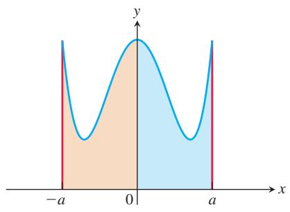
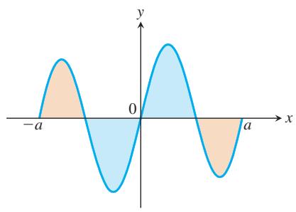
The Substitution Formula in Theorem 7 simplifies the calculation of definite integrals of even and odd functions (Section 1.1) over a symmetric interval
(b)
FIGURE 5.24 (a) For
THEOREM 8 Let
(a) If
(b) If
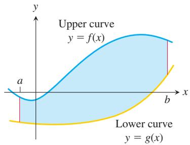
FIGURE 5.25 The region between the curves
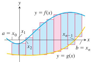
FIGURE 5.26 We approximate the region with rectangles perpendicular to the x-axis.
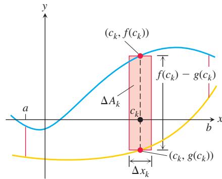
FIGURE 5.27 The area
Proof of Part (a)
The proof of part (b) is similar, and you are asked to give it in Exercise 120.
EXAMPLE 3 Evaluate
Solution Since
Areas Between Curves
Suppose we want to find the area of a region that is bounded above by the curve
To see what the integral should be, we first approximate the region with n vertical rectangles based on a partition
We then approximate the area of the region by adding the areas of the n rectangles:
As
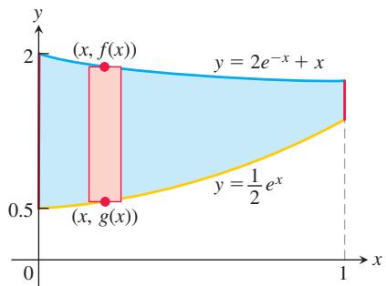
FIGURE 5.28 The region in Example 4 with a typical approximating rectangle.
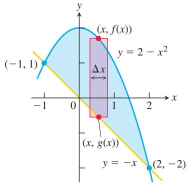
FIGURE 5.29 The region in Example 5 with a typical approximating rectangle from a Riemann sum.
DEFINITION If f and g are continuous with
throughout [a, b], then the area of the region between the curves 𝑓 ( 𝑥 ) ≥ 𝑔 ( 𝑥 ) and 𝑦 = 𝑓 ( 𝑥 ) from a to b is the integral of 𝑦 = 𝑔 ( 𝑥 ) from a to b: ( 𝑓 − 𝑔 ) 𝐴 = ∫ 𝑏 𝑎 [ 𝑓 ( 𝑥 ) − 𝑔 ( 𝑥 ) ] 𝑑 𝑥 .
When applying this definition it is usually helpful to graph the curves. The graph reveals which curve is the upper curve f and which is the lower curve g. It also helps you find the limits of integration if they are not given. You may need to find where the curves intersect to determine the limits of integration, and this may involve solving the equation
EXAMPLE 4 Find the area of the region bounded above by the curve
Solution Figure 5.28 displays the graphs of the curves and the region whose area we want to find. The area between the curves over the interval
EXAMPLE 5 Find the area of the region enclosed by the parabola
Solution First we sketch the two curves (Figure 5.29). The limits of integration are found by solving
The region runs from
If the formula for a bounding curve changes at one or more points, we subdivide the region into subregions that correspond to the formula changes and apply the formula for the area between curves to each subregion.
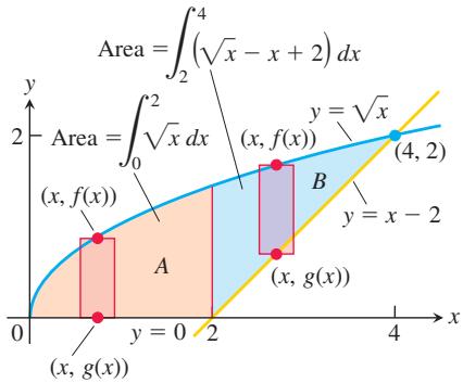
FIGURE 5.30 When the formula for a bounding curve changes, the area integral changes to become the sum of integrals to match, one integral for each of the shaded regions shown here for Example 6.
EXAMPLE 6 Find the area of the region in the first quadrant that is bounded above by
Solution Figure 5.30 shows that the region’s upper boundary is the graph of
The limits of integration for region A are a = 0 and b = 2. The left-hand limit for region B is a = 2. To find the right-hand limit, we solve the equations
Only the value x = 4 satisfies the equation
We add the areas of subregions A and B to find the total area:
Integration with Respect to y
If a region’s bounding curves are described by functions of
To find the areas of regions like these:
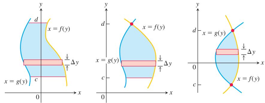
use the formula
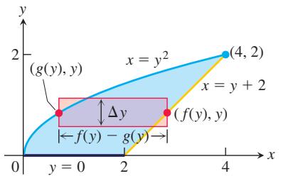
FIGURE 5.31 It takes two integrations to find the area of this region if we integrate with respect to x. It takes only one if we integrate with respect to y (Example 7).
In this equation
EXAMPLE 7 Find the area of the region in Example 6 by integrating with respect to y.
Solution We first sketch the region and a typical horizontal rectangle based on a partition of an interval of
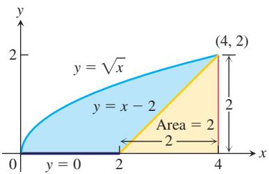
FIGURE 5.32 The area of the blue region is the area under the parabola
The upper limit of integration is
The area of the region is
This is the result of Example 6, found with less work.
Although it was easier to find the area in Example 6 by integrating with respect to y rather than x (as we did in Example 7), there is an easier way yet. Looking at Figure 5.32, we see that the area we want is the area between the curve
EXERCISES 5.6
Evaluating Definite Integrals
Evaluating Definite Integrals
Use the Substitution Formula in Theorem 7 to evaluate the integrals in Exercises 1–48.
2. a.
- a.
∫ 𝜋 0 3 c o s 2 𝑥 s i n 𝑥 𝑑 𝑥
b.
- a.
∫ 1 0 𝑡 3 ( 1 + 𝑡 4 ) 3 𝑑 𝑡
b.
- a.
∫ √ 7 0 𝑡 ( 𝑡 2 + 1 ) 1 / 3 𝑑 𝑡
b.
- a.
∫ 1 − 1 5 𝑟 ( 4 + 𝑟 2 ) 2 𝑑 𝑟
b.
- a.
∫ 1 0 1 0 √ 𝑣 ( 1 + 𝑣 3 / 2 ) 2 𝑑 𝑣
b.
- a.
∫ √ 3 0 4 𝑥 √ 𝑥 2 + 1 𝑑 𝑥
b.
- a.
∫ 1 0 𝑥 3 √ 𝑥 4 + 9 𝑑 𝑥
b.
- a.
∫ 1 0 𝑡 √ 4 + 5 𝑡 𝑑 𝑡
b.
-
a.
∫ 𝜋 / 6 0 ( 1 − c o s 3 𝑡 ) s i n 3 𝑡 𝑑 𝑡 -
a.
∫ 2 𝜋 0 c o s 𝑧 √ 4 + 3 s i n 𝑧 𝑑 𝑧 ∫ 𝜋 − 𝜋 c o s 𝑧 √ 4 + 3 s i n 𝑧 𝑑 𝑧
Area
-
a.
∫ 0 − 𝜋 / 2 ( 2 + t a n 𝑡 2 ) s e c 2 𝑡 2 𝑑 𝑡
b.
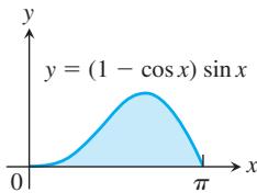
-
∫ 1 0 √ 𝑡 5 + 2 𝑡 ( 5 𝑡 4 + 2 ) 𝑑 𝑡 -
∫ 4 1 𝑑 𝑦 2 √ 𝑦 ( 1 + √ 𝑦 ) 2 -
∫ 𝜋 / 6 0 c o s − 3 2 𝜃 s i n 2 𝜃 𝑑 𝜃 -
∫ 3 𝜋 / 2 𝜋 c o t 5 ( 𝜃 6 ) s e c 2 ( 𝜃 6 ) 𝑑 𝜃 -
∫ 𝜋 0 5 ( 5 − 4 c o s 𝑡 ) 1 / 4 s i n 𝑡 𝑑 𝑡 -
∫ 𝜋 / 4 0 ( 1 − s i n 2 𝑡 ) 3 / 2 c o s 2 𝑡 𝑑 𝑡
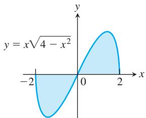
-
∫ 1 0 ( 4 𝑦 − 𝑦 2 + 4 𝑦 3 + 1 ) − 2 / 3 ( 1 2 𝑦 2 − 2 𝑦 + 4 ) 𝑑 𝑦 -
∫ 1 0 ( 𝑦 3 + 6 𝑦 2 − 1 2 𝑦 + 9 ) − 1 / 2 ( 𝑦 2 + 4 𝑦 − 4 ) 𝑑 𝑦 -
∫ 3 √ 𝜋 2 0 √ 𝜃 c o s 2 ( 𝜃 3 / 2 ) 𝑑 𝜃 -
∫ − 1 / 2 − 1 𝑡 − 2 s i n 2 ( 1 + 1 𝑡 ) 𝑑 𝑡
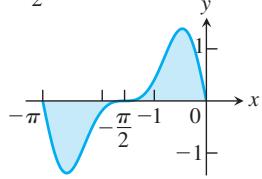
-
∫ 𝜋 / 4 0 ( 1 + 𝑒 t a n 𝜃 ) s e c 2 𝜃 𝑑 𝜃 -
∫ 𝜋 / 2 𝜋 / 4 ( 1 + 𝑒 c o t 𝜃 ) c s c 2 𝜃 𝑑 𝜃 -
∫ 𝜋 0 s i n 𝑡 2 − c o s 𝑡 𝑑 𝑡 -
∫ 𝜋 / 3 0 4 s i n 𝜃 1 − 4 c o s 𝜃 𝑑 𝜃
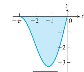
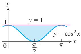
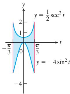
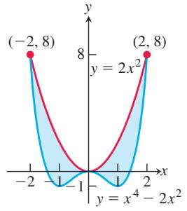
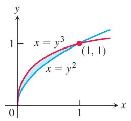
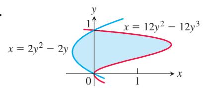
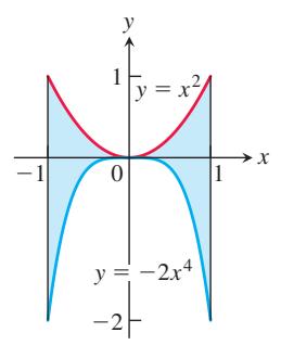
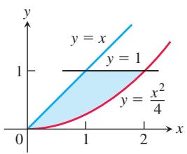
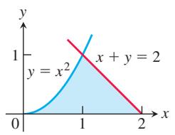
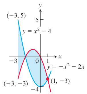
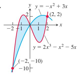
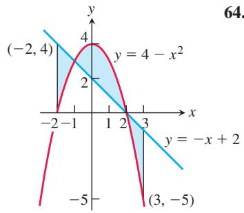
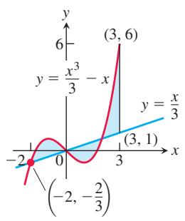
-
∫ 2 1 2 l n 𝑥 𝑥 𝑑 𝑥 -
∫ 4 2 𝑑 𝑥 𝑥 l n 𝑥 -
∫ 4 2 𝑑 𝑥 𝑥 ( l n 𝑥 ) 2 -
∫ 1 6 2 𝑑 𝑥 2 𝑥 √ l n 𝑥 -
∫ 𝜋 / 2 0 t a n 𝑥 2 𝑑 𝑥 -
∫ 𝜋 / 2 𝜋 / 4 c o t 𝑡 𝑑 𝑡 -
∫ 𝜋 / 3 0 t a n 2 𝜃 c o s 𝜃 𝑑 𝜃 -
∫ 𝜋 / 1 2 0 6 t a n 3 𝑥 𝑑 𝑥 -
∫ 𝜋 / 2 − 𝜋 / 2 2 c o s 𝜃 𝑑 𝜃 1 + ( s i n 𝜃 ) 2 -
∫ 𝜋 / 4 𝜋 / 6 c s c 2 𝑥 𝑑 𝑥 1 + ( c o t 𝑥 ) 2 -
∫ l n √ 3 0 𝑒 𝑥 𝑑 𝑥 1 + 𝑒 2 𝑥 -
∫ 𝑒 𝜋 / 4 1 4 𝑑 𝑡 𝑡 ( 1 + l n 2 𝑡 ) -
∫ 1 0 4 𝑑 𝑠 √ 4 − 𝑠 2 -
∫ ( 3 / 4 ) √ 2 0 𝑑 𝑠 √ 9 − 4 𝑠 2 -
∫ 2 √ 2 s e c 2 ( s e c − 1 𝑥 ) 𝑑 𝑥 𝑥 √ 𝑥 2 − 1 -
∫ 2 2 / √ 3 c o s ( s e c − 1 𝑥 ) 𝑑 𝑥 𝑥 √ 𝑥 2 − 1 -
∫ − √ 2 / 2 − 1 𝑑 𝑦 𝑦 √ 4 𝑦 2 − 1 -
∫ 3 0 𝑦 𝑑 𝑦 √ 5 𝑦 + 1
b.
-
∫ 1 0 t a n − 1 𝑥 1 + 𝑥 2 𝑑 𝑥 -
∫ 1 / √ 3 − √ 3 c o s ( t a n − 1 3 𝑥 ) 1 + 9 𝑥 2 𝑑 𝑥
Find the total areas of the shaded regions in Exercises 49–64.
𝑦 = 𝜋 2 ( c o s 𝑥 ) ( s i n ( 𝜋 + 𝜋 𝑦 s i n 𝑥 ) )
Find the areas of the regions enclosed by the lines and curves in Exercises 65–74.
𝑦 = 𝑥 2 − 2 𝑦 = 2
-
𝑦 = 𝑥 2 a n d 𝑦 = − 𝑥 2 + 4 𝑥 -
𝑦 = 7 − 2 𝑥 2 a n d 𝑦 = 𝑥 2 + 4 -
𝑦 = 𝑥 4 − 4 𝑥 2 + 4 a n d 𝑦 = 𝑥 2 -
𝑦 = 𝑥 √ 𝑎 2 − 𝑥 2 𝑎 > 0 𝑦 = 0 -
𝑦 = √ | 𝑥 | 5 𝑦 = 𝑥 + 6 -
𝑦 = | 𝑥 2 − 4 | a n d 𝑦 = ( 𝑥 2 / 2 ) + 4
Find the areas of the regions enclosed by the lines and curves in Exercises 75–82.
-
𝑥 = 2 𝑦 2 , 𝑥 = 0 , a n d 𝑦 = 3 -
𝑥 = 𝑦 2 a n d 𝑥 = 𝑦 + 2 -
𝑦 2 − 4 𝑥 = 4 a n d 4 𝑥 − 𝑦 = 1 6 -
𝑥 − 𝑦 2 = 0 a n d 𝑥 + 2 𝑦 2 = 3 -
𝑥 + 𝑦 2 = 0 a n d 𝑥 + 3 𝑦 2 = 2 -
𝑥 − 𝑦 2 / 3 = 0 a n d 𝑥 + 𝑦 4 = 2 -
𝑥 = 𝑦 2 − 1 a n d 𝑥 = | 𝑦 | √ 1 − 𝑦 2 -
𝑥 = 𝑦 3 − 𝑦 2 a n d 𝑥 = 2 𝑦
Find the areas of the regions enclosed by the curves in Exercises 83–86.
-
4 𝑥 2 + 𝑦 = 4 a n d 𝑥 4 − 𝑦 = 1 -
𝑥 3 − 𝑦 = 0 a n d 3 𝑥 2 − 𝑦 = 4 -
𝑥 + 4 𝑦 2 = 4 a n d 𝑥 + 𝑦 4 = 1 , f o r 𝑥 ≥ 0 -
𝑥 + 𝑦 2 = 3 a n d 4 𝑥 + 𝑦 2 = 0
Find the areas of the regions enclosed by the lines and curves in Exercises 87–94.
-
𝑦 = 2 s i n 𝑥 a n d 𝑦 = s i n 2 𝑥 , 0 ≤ 𝑥 ≤ 𝜋 -
𝑦 = 8 c o s 𝑥 a n d 𝑦 = s e c 2 𝑥 , − 𝜋 / 3 ≤ 𝑥 ≤ 𝜋 / 3 -
𝑦 = c o s ( 𝜋 𝑥 / 2 ) a n d 𝑦 = 1 − 𝑥 2 -
𝑦 = s i n ( 𝜋 𝑥 / 2 ) a n d 𝑦 = 𝑥 -
𝑦 = s e c 2 𝑥 , 𝑦 = t a n 2 𝑥 , 𝑥 = − 𝜋 / 4 , a n d 𝑥 = 𝜋 / 4 -
𝑥 = t a n 2 𝑦 a n d 𝑥 = − t a n 2 𝑦 , − 𝜋 / 4 ≤ 𝑦 ≤ 𝜋 / 4 -
𝑥 = 3 s i n 𝑦 √ c o s 𝑦 a n d 𝑥 = 0 , 0 ≤ 𝑦 ≤ 𝜋 / 2 -
𝑦 = s e c 2 ( 𝜋 𝑥 / 3 ) a n d 𝑦 = 𝑥 1 / 3 , − 1 ≤ 𝑥 ≤ 1
Area Between Curves
-
Find the area of the propeller-shaped region enclosed by the curve
𝑥 − 𝑦 3 = 0 -
Find the area of the propeller-shaped region enclosed by the curves
𝑥 − 𝑦 1 / 3 = 0 𝑥 − 𝑦 1 / 5 = 0 -
Find the area of the region in the first quadrant bounded by the line
𝑦 = 𝑥 𝑥 = 2 𝑦 = 1 / 𝑥 2 𝑥 -
Find the area of the “triangular” region in the first quadrant bounded on the left by the y-axis and on the right by the curves
𝑦 = s i n 𝑥 𝑦 = c o s 𝑥 -
Find the area between the curves
𝑦 = l n 𝑥 𝑦 = l n 2 𝑥 𝑥 = 1 𝑥 = 5 -
Find the area between the curve
𝑦 = t a n 𝑥 𝑥 𝑥 = − 𝜋 / 4 𝑥 = 𝜋 / 3 -
Find the area of the “triangular” region in the first quadrant that is bounded above by the curve
𝑦 = 𝑒 2 𝑥 𝑦 = 𝑒 𝑥 𝑥 = l n 3 -
Find the area of the “triangular” region in the first quadrant that is bounded above by the curve
𝑦 = 𝑒 𝑥 / 2 𝑦 = 𝑒 − 𝑥 / 2 𝑥 = 2 l n 2 -
Find the area of the region between the curve
𝑦 = 2 𝑥 / ( 1 + 𝑥 2 ) − 2 ≤ 𝑥 ≤ 2 𝑥 -
Find the area of the region between the curve
𝑦 = 2 1 − 𝑥 − 1 ≤ 𝑥 ≤ 1 -
The region bounded below by the parabola
𝑦 = 𝑥 2
a. Sketch the region and draw a line y = c across it that looks about right. In terms of c, what are the coordinates of the points where the line and parabola intersect? Add them to your figure.
b. Find
c. Find c by integrating with respect to x. (This puts c into the integrand as well.)
-
Find the area of the region between the curve
𝑦 = 3 − 𝑥 2 𝑦 = − 1 𝑥 𝑦 -
Find the area of the region in the first quadrant bounded on the left by the
𝑦 𝑦 = 𝑥 / 4 𝑦 = 1 + √ 𝑥 𝑦 = 2 / √ 𝑥 -
Find the area of the region in the first quadrant bounded on the left by the y-axis, below by the curve
𝑥 = 2 √ 𝑦 𝑥 = ( 𝑦 − 1 ) 2
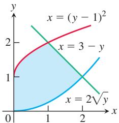
- The figure here shows triangle
𝐴 𝑂 𝐶 𝑦 = 𝑥 2 𝑦 = 𝑎 2 𝑎
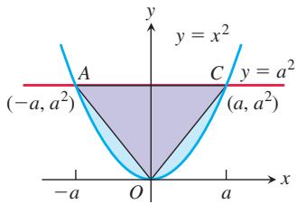
-
Suppose the area of the region between the graph of a positive continuous function
𝑓 𝑥 𝑥 = 𝑎 𝑥 = 𝑏 𝑦 = 𝑓 ( 𝑥 ) 𝑦 = 2 𝑓 ( 𝑥 ) 𝑥 = 𝑎 𝑥 = 𝑏 -
Which of the following integrals, if either, calculates the area of the shaded region shown here? Give reasons for your answer.
b.
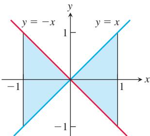
- True, sometimes true, or never true? The area of the region between the graphs of the continuous functions
𝑦 = 𝑓 ( 𝑥 ) 𝑦 = 𝑔 ( 𝑥 ) 𝑥 = 𝑎 𝑥 = 𝑏 ( 𝑎 < 𝑏 )
Give reasons for your answer.
Comparing Areas
Compute the areas of the light blue and dark blue regions in each of Exercises 113 to 116 and determine which is larger, or show that they have equal area.
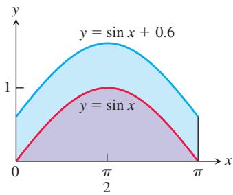
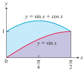
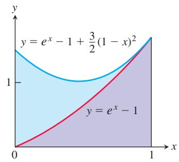
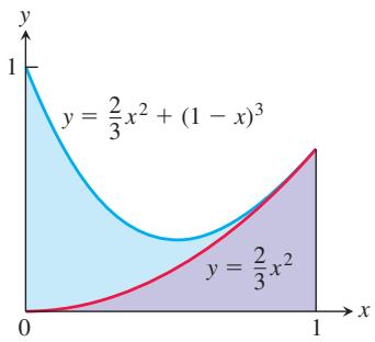
Theory and Examples
- Suppose that
𝐹 ( 𝑥 ) 𝑓 ( 𝑥 ) = ( s i n 𝑥 ) / 𝑥 𝑥 > 0
in terms of
- Show that if
𝑓
Find
if a. f is odd, b. f is even.
- a. Show that if f is odd on
[ − 𝑎 , 𝑎 ]
b. Test the result in part (a) with
- If f is a continuous function, find the value of the integral
by making the substitution
- By using a substitution, prove that for all positive numbers x and y,
The Shift Property for Definite Integrals A basic property of definite integrals is their invariance under translation, as expressed by the equation
The equation holds whenever
because the areas of the shaded regions are congruent.
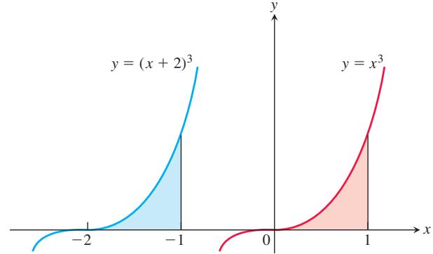
-
Use a substitution to verify Equation (1).
-
For each of the following functions, graph
𝑓 ( 𝑥 ) [ 𝑎 , 𝑏 ] 𝑓 ( 𝑥 + 𝑐 ) [ 𝑎 − 𝑐 , 𝑏 − 𝑐 ]
a.
b.
c.
COMPUTER EXPLORATIONS
In Exercises 125–128, you will find the area between curves in the plane when you cannot find their points of intersection using simple algebra. Use a CAS to perform the following steps:
a. Plot the curves together to see what they look like and how many points of intersection they have.
b. Use the numerical equation solver in your CAS to find all the points of intersection.
c. Integrate
d. Sum together the integrals found in part (c).
-
𝑓 ( 𝑥 ) = 𝑥 3 3 − 𝑥 2 2 − 2 𝑥 + 1 3 , 𝑔 ( 𝑥 ) = 𝑥 − 1 -
𝑓 ( 𝑥 ) = 𝑥 4 2 − 3 𝑥 3 + 1 0 , 𝑔 ( 𝑥 ) = 8 − 1 2 𝑥 -
𝑓 ( 𝑥 ) = 𝑥 + s i n ( 2 𝑥 ) 𝑔 ( 𝑥 ) = 𝑥 3 -
𝑓 ( 𝑥 ) = 𝑥 2 c o s 𝑥 , 𝑔 ( 𝑥 ) = 𝑥 3 − 𝑥
CHAPTER 5 Questions to Guide Your Review
-
How can you sometimes estimate quantities like distance traveled, area, and average value with finite sums? Why might you want to do so?
-
What is sigma notation? What advantage does it offer? Give examples.
-
What is a Riemann sum? Why might you want to consider such a sum?
-
What is the norm of a partition of a closed interval?
-
What is the definite integral of a function
𝑓 [ 𝑎 , 𝑏 ] -
What is the relation between definite integrals and area? Describe some other interpretations of definite integrals.
-
What is the average value of an integrable function over a closed interval? Must the function assume its average value? Explain.
-
Describe the rules for working with definite integrals (Table 5.6). Give examples.
-
What is the Fundamental Theorem of Calculus? Why is it so important? Illustrate each part of the theorem with an example.
-
What is the Net Change Theorem? What does it say about the integral of velocity? The integral of marginal cost?
-
Discuss how the processes of integration and differentiation can be considered as “inverses” of each other.
-
How does the Fundamental Theorem provide a solution to the initial value problem
𝑑 𝑦 / 𝑑 𝑥 = 𝑓 ( 𝑥 ) 𝑦 ( 𝑥 0 ) = 𝑦 0 -
How is integration by substitution related to the Chain Rule?
-
How can you sometimes evaluate indefinite integrals by substitution? Give examples.
-
How does the method of substitution work for definite integrals? Give examples.
-
How do you define and calculate the area of the region between the graphs of two continuous functions? Give an example.
CHAPTER 5 Practice Exercises
Finite Sums and Estimates
- The accompanying figure shows the graph of the velocity (m/s) of a model rocket for the first 8 s after launch. The rocket accelerated straight up for the first 2 s and then coasted to reach its maximum height at t = 8 s.
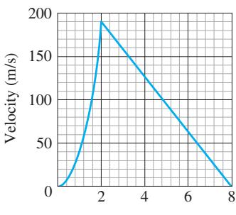
Time after launch (s)
a. Assuming that the rocket was launched from ground level, about how high did it go? (This is the rocket in Section 3.4, Exercise 17, but you do not need to do Exercise 17 to do the exercise here.)
b. Sketch a graph of the rocket’s height above ground as a function of time for
- a. The accompanying figure shows the velocity (m/s) of a body moving along the s-axis during the time interval from t = 0 to t = 10 s. About how far did the body travel during those 10 s?
b. Sketch a graph of
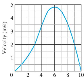
Time (s)
-
Suppose that
∑ 1 0 𝑘 = 1 𝑎 𝑘 = − 2 ∑ 1 0 𝑘 = 1 𝑏 𝑘 = 2 5 ∑ 1 0 𝑘 = 1 𝑎 𝑘 4 ∑ 1 0 𝑘 = 1 ( 𝑏 𝑘 − 3 𝑎 𝑘 ) ∑ 1 0 𝑘 = 1 ( 𝑎 𝑘 + 𝑏 𝑘 − 1 ) ∑ 1 0 𝑘 = 1 ( 5 2 − 𝑏 𝑘 ) -
Suppose that
∑ 2 0 𝑘 = 1 𝑎 𝑘 = 0 ∑ 2 0 𝑘 = 1 𝑏 𝑘 = 7 ∑ 2 0 𝑘 = 1 3 𝑎 𝑘 ∑ 2 0 𝑘 = 1 ( 𝑎 𝑘 + 𝑏 𝑘 ) ∑ 2 0 𝑘 = 1 ( 1 2 − 2 𝑏 𝑘 7 ) ∑ 2 0 𝑘 = 1 ( 𝑎 𝑘 − 2 )
Definite Integrals
In Exercises 5–8, express each limit as a definite integral. Then evaluate the integral to find the value of the limit. In each case, P is a partition of the given interval, and the numbers
-
l i m ‖ 𝑃 ‖ → 0 ∑ 𝑛 𝑘 = 1 ( 2 𝑐 𝑘 − 1 ) − 1 / 2 Δ 𝑥 𝑘 𝑃 -
l i m ‖ 𝑃 ‖ → 0 ∑ 𝑛 𝑘 = 1 𝑐 𝑘 ( 𝑐 2 𝑘 − 1 ) 1 / 3 Δ 𝑥 𝑘 𝑃 -
l i m ‖ 𝑃 ‖ → 0 ∑ 𝑛 𝑘 = 1 ( c o s ( 𝑐 𝑘 2 ) ) Δ 𝑥 𝑘 𝑃 [ − 𝜋 , 0 ] -
l i m ‖ 𝑃 ‖ → 0 ∑ 𝑛 𝑘 = 1 ( s i n 𝑐 𝑘 ) ( c o s 𝑐 𝑘 ) Δ 𝑥 𝑘 [ 0 , 𝜋 / 2 ] -
If
∫ 2 − 2 3 𝑓 ( 𝑥 ) 𝑑 𝑥 = 1 2 ∫ 5 − 2 𝑓 ( 𝑥 ) 𝑑 𝑥 = 6 ∫ 5 − 2 𝑔 ( 𝑥 ) 𝑑 𝑥 = 2 ∫ 2 − 2 𝑓 ( 𝑥 ) 𝑑 𝑥 ∫ 5 2 𝑓 ( 𝑥 ) 𝑑 𝑥 ∫ − 2 5 𝑔 ( 𝑥 ) 𝑑 𝑥 ∫ 5 − 2 ( − 𝜋 𝑔 ( 𝑥 ) ) 𝑑 𝑥 ∫ 5 − 2 ( 𝑓 ( 𝑥 ) + 𝑔 ( 𝑥 ) 5 ) 𝑑 𝑥 -
If
∫ 2 0 𝑓 ( 𝑥 ) 𝑑 𝑥 = 𝜋 , ∫ 2 0 7 𝑔 ( 𝑥 ) 𝑑 𝑥 = 7 ∫ 1 0 𝑔 ( 𝑥 ) 𝑑 𝑥 = 2
a.∫ 2 0 𝑔 ( 𝑥 ) 𝑑 𝑥 ∫ 2 1 𝑔 ( 𝑥 ) 𝑑 𝑥 ∫ 0 2 𝑓 ( 𝑥 ) 𝑑 𝑥 ∫ 2 0 √ 2 𝑓 ( 𝑥 ) 𝑑 𝑥 ∫ 2 0 ( 𝑔 ( 𝑥 ) − 3 𝑓 ( 𝑥 ) ) 𝑑 𝑥
Area
In Exercises 11–14, find the total area of the region between the graph of f and the x-axis.
-
𝑓 ( 𝑥 ) = 𝑥 2 − 4 𝑥 + 3 , 0 ≤ 𝑥 ≤ 3 -
𝑓 ( 𝑥 ) = 1 − ( 𝑥 2 / 4 ) , − 2 ≤ 𝑥 ≤ 3 -
𝑓 ( 𝑥 ) = 5 − 5 𝑥 2 / 3 , − 1 ≤ 𝑥 ≤ 8 -
𝑓 ( 𝑥 ) = 1 − √ 𝑥 , 0 ≤ 𝑥 ≤ 4
Find the areas of the regions enclosed by the curves and lines in Exercises 15–26.
-
𝑦 = 𝑥 , 𝑦 = 1 / 𝑥 2 , 𝑥 = 2 -
𝑦 = 𝑥 , 𝑦 = 1 / √ 𝑥 , 𝑥 = 2 -
√ 𝑥 + √ 𝑦 = 1 𝑥 = 0 , 𝑦 = 0
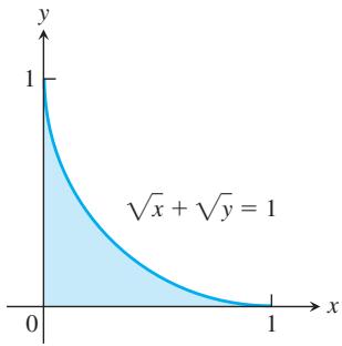
𝑥 3 + √ 𝑦 = 1 , 𝑥 = 0 , 𝑦 = 0 , 𝑓 𝑜 𝑟 0 ≤ 𝑥 ≤ 1
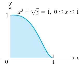
-
𝑥 = 2 𝑦 2 𝑥 = 0 𝑦 = 3 -
𝑥 = 4 − 𝑦 2 𝑥 = 0 -
𝑦 2 = 4 𝑥 , 𝑦 = 4 𝑥 − 2 -
𝑦 2 = 4 𝑥 + 4 , 𝑦 = 4 𝑥 − 1 6 -
𝑦 = s i n 𝑥 , 𝑦 = 𝑥 , 0 ≤ 𝑥 ≤ 𝜋 / 4 -
𝑦 = | s i n 𝑥 | 𝑦 = 1 − 𝜋 / 2 ≤ 𝑥 ≤ 𝜋 / 2 -
𝑦 = 2 s i n 𝑥 , 𝑦 = s i n 2 𝑥 , 0 ≤ 𝑥 ≤ 𝜋 -
𝑦 = 8 c o s 𝑥 , 𝑦 = s e c 2 𝑥 , − 𝜋 / 3 ≤ 𝑥 ≤ 𝜋 / 3 -
Find the area of the “triangular” region bounded on the left by
𝑥 + 𝑦 = 2 𝑦 = 𝑥 2 -
Find the area of the “triangular” region bounded on the left by
𝑦 = √ 𝑥 -
Find the extreme values of
𝑓 ( 𝑥 ) = 𝑥 3 − 3 𝑥 2 𝑓 𝑥 -
Find the area of the region cut from the first quadrant by the curve
𝑥 1 / 2 + 𝑦 1 / 2 = 𝑎 1 / 2 -
Find the total area of the region enclosed by the curve
𝑥 = 𝑦 2 / 3 𝑥 = 𝑦 𝑦 = − 1 -
Find the total area of the region between the curves
𝑦 = s i n 𝑥 𝑦 = c o s 𝑥 0 ≤ 𝑥 ≤ 3 𝜋 / 2 -
Find the area between the curve
𝑦 = 2 ( l n 𝑥 ) / 𝑥 -
a. Show that the area between the curve y = 1/x and the x-axis from x = 10 to x = 20 is the same as the area between the curve and the x-axis from x = 1 to x = 2.
b. Show that the area between the curve y = 1/x and the x-axis from ka to kb is the same as the area between the curve and the x-axis from x = a to x = b (0 < a < b, k > 0).
Initial Value Problems
- Show that
𝑦 = 𝑥 2 + ∫ 𝑥 1 1 𝑡 𝑑 𝑡
- Show that
𝑦 = ∫ 𝑥 0 ( 1 + 2 √ s e c 𝑡 ) 𝑑 𝑡
Express the solutions of the initial value problems in Exercises 37 and 38 in terms of integrals.
-
𝑑 𝑦 𝑑 𝑥 = s i n 𝑥 𝑥 , 𝑦 ( 5 ) = − 3 -
𝑑 𝑦 𝑑 𝑥 = √ 2 − s i n 2 𝑥 , 𝑦 ( − 1 ) = 2
Solve the initial value problems in Exercises 39–42.
-
𝑑 𝑦 𝑑 𝑥 = 1 √ 1 − 𝑥 2 , 𝑦 ( 0 ) = 0 -
𝑑 𝑦 𝑑 𝑥 = 1 𝑥 2 + 1 − 1 , 𝑦 ( 0 ) = 1 -
𝑑 𝑦 𝑑 𝑥 = 1 𝑥 √ 𝑥 2 − 1 , 𝑥 > 1 ; 𝑦 ( 2 ) = 𝜋 -
𝑑 𝑦 𝑑 𝑥 = 1 1 + 𝑥 2 − 2 √ 1 − 𝑥 2 , 𝑦 ( 0 ) = 2 -
∫ 4 1 ( 1 + √ 𝑢 ) 1 / 2 √ 𝑢 𝑑 𝑢
For Exercises 43 and 44, find a function
-
∫ 1 0 3 6 𝑑 𝑥 ( 2 𝑥 + 1 ) 3 -
∫ 1 0 𝑑 𝑟 3 √ ( 7 − 5 𝑟 ) 2 -
𝑓 ( 𝑥 ) = 1 + ∫ 𝑥 1 𝑡 𝑓 ( 𝑡 ) 𝑑 𝑡 -
𝑓 ( 𝑥 ) = ∫ 𝑥 0 ( 1 + 𝑓 ( 𝑡 ) 2 ) 𝑑 𝑡
Evaluating Indefinite Integrals
-
∫ 2 7 1 𝑥 − 4 / 3 𝑑 𝑥 -
∫ 1 1 / 8 𝑥 − 1 / 3 ( 1 − 𝑥 2 / 3 ) 3 / 2 𝑑 𝑥
Evaluate the integrals in Exercises 45–76.
-
∫ 1 / 2 0 𝑥 3 ( 1 + 9 𝑥 4 ) − 3 / 2 𝑑 𝑥 -
∫ 1 0 ( 8 𝑠 3 − 1 2 𝑠 2 + 5 ) 𝑑 𝑠 -
∫ 𝜋 0 s i n 2 5 𝑟 𝑑 𝑟 -
∫ 2 ( c o s 𝑥 ) − 1 / 2 s i n 𝑥 𝑑 𝑥 -
∫ ( t a n 𝑥 ) − 3 / 2 s e c 2 𝑥 𝑑 𝑥 -
∫ 𝜋 / 4 0 c o s 2 ( 4 𝑡 − 𝜋 4 ) 𝑑 𝑡 -
∫ 4 1 𝑑 𝑡 𝑡 √ 𝑡 -
∫ ( 2 𝜃 + 1 + 2 c o s ( 2 𝜃 + 1 ) ) 𝑑 𝜃 -
∫ 𝜋 / 3 0 s e c 2 𝜃 𝑑 𝜃 -
∫ 3 𝜋 / 4 𝜋 / 4 c s c 2 𝑥 𝑑 𝑥
Evaluating Definite Integrals
-
∫ ( 1 √ 2 𝜃 − 𝜋 + 2 s e c 2 ( 2 𝜃 − 𝜋 ) ) 𝑑 𝜃 -
∫ 3 𝜋 𝜋 c o t 2 𝑥 6 𝑑 𝑥 -
∫ ( 𝑡 − 2 𝑡 ) ( 𝑡 + 2 𝑡 ) 𝑑 𝑡 -
∫ 𝜋 0 t a n 2 𝜃 3 𝑑 𝜃 -
∫ ( 𝑡 + 1 ) 2 − 1 𝑡 4 𝑑 𝑡 -
∫ 0 − 𝜋 / 3 s e c 𝑥 t a n 𝑥 𝑑 𝑥 -
∫ √ 𝑡 s i n ( 2 𝑡 3 / 2 ) 𝑑 𝑡 -
∫ 3 𝜋 / 4 𝜋 / 4 c s c 𝑧 c o t 𝑧 𝑑 𝑧 -
∫ 2 1 4 𝑣 2 𝑑 𝑣 -
∫ ( s e c 𝜃 t a n 𝜃 ) √ 1 + s e c 𝜃 𝑑 𝜃 -
∫ 𝜋 / 2 0 5 ( s i n 𝑥 ) 3 / 2 c o s 𝑥 𝑑 𝑥 -
∫ 𝜋 / 2 − 𝜋 / 2 1 5 s i n 4 3 𝑥 c o s 3 𝑥 𝑑 𝑥 -
∫ 𝑒 𝑥 s e c 2 ( 𝑒 𝑥 − 7 ) 𝑑 𝑥
Evaluate the integrals in Exercises 77–116.
-
∫ 𝜋 / 4 0 s e c 2 𝑥 ( 1 + 7 t a n 𝑥 ) 2 / 3 𝑑 𝑥 -
∫ 𝜋 / 2 0 3 s i n 𝑥 c o s 𝑥 √ 1 + 3 s i n 2 𝑥 𝑑 𝑥 -
∫ 1 − 1 ( 3 𝑥 2 − 4 𝑥 + 7 ) 𝑑 𝑥 -
∫ 𝑒 𝑦 c s c ( 𝑒 𝑦 + 1 ) c o t ( 𝑒 𝑦 + 1 ) 𝑑 𝑦 -
∫ 8 1 ( 2 3 𝑥 − 8 𝑥 2 ) 𝑑 𝑥 -
∫ ( c s c 2 𝑥 ) 𝑒 c o t 𝑥 𝑑 𝑥 -
∫ ( s e c 2 𝑥 ) 𝑒 t a n 𝑥 𝑑 𝑥 -
∫ 4 1 ( 𝑥 8 + 1 2 𝑥 ) 𝑑 𝑥 -
∫ 𝑒 1 √ l n 𝑥 𝑥 𝑑 𝑥 -
∫ 0 − l n 2 𝑒 2 𝑤 𝑑 𝑤 -
∫ 1 − 1 𝑑 𝑥 3 𝑥 − 4 -
∫ t a n ( l n 𝑣 ) 𝑣 𝑑 𝑣 -
∫ − 1 − 2 𝑒 − ( 𝑥 + 1 ) 𝑑 𝑥 -
∫ 4 0 2 𝑡 𝑡 2 − 2 5 𝑑 𝑡 -
∫ l n 9 0 𝑒 𝜃 ( 𝑒 𝜃 − 1 ) 1 / 2 𝑑 𝜃 -
∫ 1 𝑟 c s c 2 ( 1 + l n 𝑟 ) 𝑑 𝑟 -
∫ ( l n 𝑥 ) − 3 𝑥 𝑑 𝑥 -
∫ 3 1 ( l n ( 𝑣 + 1 ) ) 2 𝑣 + 1 𝑑 𝑣 -
∫ 2 t a n 𝑥 s e c 2 𝑥 𝑑 𝑥 -
∫ l n 5 0 𝑒 𝑟 ( 3 𝑒 𝑟 + 1 ) − 3 / 2 𝑑 𝑟 -
∫ 𝑥 3 𝑥 2 𝑑 𝑥 -
∫ 6 𝑑 𝑟 √ 4 − ( 𝑟 + 1 ) 2 -
∫ 3 𝑑 𝑟 √ 1 − 4 ( 𝑟 − 1 ) 2 -
∫ 𝑒 1 8 l n 3 l o g 3 𝜃 𝜃 𝑑 𝜃 -
∫ 𝑑 𝑥 1 + ( 3 𝑥 + 1 ) 2 -
∫ c o s 𝜃 ⋅ s i n ( s i n 𝜃 ) 𝑑 𝜃 -
∫ 𝑑 𝑥 ( 𝑥 + 3 ) √ ( 𝑥 + 3 ) 2 − 2 5 -
∫ 𝑑 𝑥 ( 2 𝑥 − 1 ) √ ( 2 𝑥 − 1 ) 2 − 4 -
∫ 𝑑 𝑥 2 + ( 𝑥 − 1 ) 2 -
∫ ( a r c t a n 𝑥 ) 2 𝑑 𝑥 1 + 𝑥 2 -
∫ 1 / 5 − 1 / 5 6 𝑑 𝑥 √ 4 − 2 5 𝑥 2 -
∫ 𝑒 1 1 𝑥 ( 1 + 7 l n 𝑥 ) − 1 / 3 𝑑 𝑥 -
∫ √ a r c s i n 𝑥 𝑑 𝑥 √ 1 − 𝑥 2 -
∫ 𝑒 a r c s i n √ 𝑥 𝑑 𝑥 2 √ 𝑥 − 𝑥 2 -
∫ 𝑑 𝑦 √ a r c t a n 𝑦 ( 1 + 𝑦 2 ) -
∫ 3 √ 3 𝑑 𝑡 3 + 𝑡 2 -
∫ s i n 2 𝜃 − c o s 2 𝜃 ( s i n 2 𝜃 + c o s 2 𝜃 ) 3 𝑑 𝜃 -
∫ 8 1 l o g 4 𝜃 𝜃 𝑑 𝜃 -
∫ 8 4 √ 2 2 4 𝑑 𝑦 𝑦 √ 𝑦 2 − 1 6 -
∫ 3 / 4 − 3 / 4 6 𝑑 𝑥 √ 9 − 4 𝑥 2 -
∫ 2 − 2 3 𝑑 𝑡 4 + 3 𝑡 2 -
∫ − √ 6 / √ 5 − 2 / √ 5 𝑑 𝑦 | 𝑦 | √ 5 𝑦 2 − 3 -
∫ 1 1 / √ 3 𝑑 𝑦 𝑦 √ 4 𝑦 2 − 1 -
∫ 2 / 3 √ 2 / 3 𝑑 𝑦 | 𝑦 | √ 9 𝑦 2 − 1
Average Values
-
Find the average value of
𝑓 ( 𝑥 ) = 𝑚 𝑥 + 𝑏 [ − 1 , 1 ] [ − 𝑘 , 𝑘 ] -
Find the average value of a.
𝑦 = √ 3 𝑥 𝑦 = √ 𝑎 𝑥 -
Let
𝑓 [ 𝑎 , 𝑏 ] 𝑓 [ 𝑎 , 𝑏 ]
and the instantaneous rate of change of f at x to be
Is this the case? Give reasons for your answer.
-
Is it true that the average value of an integrable function over an interval of length 2 is half the function’s integral over the interval? Give reasons for your answer.
-
a. Verify that
∫ l n 𝑥 𝑑 𝑥 = 𝑥 l n 𝑥 − 𝑥 + 𝐶
b. Find the average value of
- Find the average value of
𝑓 ( 𝑥 ) = 1 / 𝑥
T 123. Compute the average value of the temperature function
for a 365-day year. (See Exercise 98, Section 3.6.) This is one way to estimate the annual mean air temperature in Fairbanks, Alaska. The National Weather Service’s official figure, a numerical average of the daily normal mean air temperatures for the year, is
T 124. Specific heat of a gas Specific heat
Find the average value of
Differentiating Integrals
In Exercises 125–132, find dy/dx.
-
𝑦 = ∫ 𝑥 2 √ 2 + c o s 3 𝑡 𝑑 𝑡 -
𝑦 = ∫ 7 𝑥 2 2 √ 2 + c o s 3 𝑡 𝑑 𝑡 -
𝑦 = ∫ 1 𝑥 6 3 + 𝑡 4 𝑑 𝑡 -
𝑦 = ∫ 2 s e c 𝑥 1 𝑡 2 + 1 𝑑 𝑡 -
𝑦 = ∫ 0 l n 𝑥 2 𝑒 c o s 𝑡 𝑑 𝑡 -
𝑦 = ∫ 𝑒 √ 𝑥 1 l n ( 𝑡 2 + 1 ) 𝑑 𝑡 -
𝑦 = ∫ s i n − 1 𝑥 0 𝑑 𝑡 √ 1 − 2 𝑡 2 -
𝑦 = ∫ 𝜋 / 4 t a n − 1 𝑥 𝑒 √ 𝑡 𝑑 𝑡
Theory and Examples
Additional and Advanced Exercises
- a. If
∫ 1 0 7 𝑓 ( 𝑥 ) 𝑑 𝑥 = 7 ∫ 1 0 𝑓 ( 𝑥 ) 𝑑 𝑥 = 1 ?
b. If
Give reasons for your answers.
CHAPTER 5
Theory and Examples
-
Is it true that every function
𝑦 = 𝑓 ( 𝑥 ) [ 𝑎 , 𝑏 ] [ 𝑎 , 𝑏 ] -
Suppose that
𝑓 ( 𝑥 ) 𝑓 ( 𝑥 ) = √ 1 + 𝑥 4 ∫ 1 0 √ 1 + 𝑥 4 𝑑 𝑥 𝐹 -
Find
𝑑 𝑦 / 𝑑 𝑥 𝑦 = ∫ 1 𝑥 √ 1 + 𝑡 2 𝑑 𝑡 -
Skydivers A and B are in a helicopter hovering at
2 0 0 0 m 2 2 0 0 m 4 . 9 m / s -
Find
𝑑 𝑦 / 𝑑 𝑥 𝑦 = ∫ 0 c o s 𝑥 ( 1 / ( 1 − 𝑡 2 ) ) 𝑑 𝑡 -
A new parking lot To meet the demand for parking, your town has allocated the area shown here. As the town engineer, you have been asked by the town council to find out if the lot can be built for
1 0 , 0 0 0 . 𝑇 ℎ 𝑒 𝑐 𝑜 𝑠 𝑡 𝑡 𝑜 𝑐 𝑙 𝑒 𝑎 𝑟 𝑡 ℎ 𝑒 𝑙 𝑎 𝑛 𝑑 𝑤 𝑖 𝑙 𝑙 𝑏 𝑒 2 . 0 0 𝑎 𝑠 𝑞 𝑢 𝑎 𝑟 𝑒 𝑚 𝑒 𝑡 𝑒 𝑟 𝑡 𝑜 𝑝 𝑎 𝑣 𝑒 . 𝐶 𝑎 𝑛 𝑡 ℎ 𝑒 𝑗 𝑜 𝑏 𝑏 𝑒 𝑑 𝑜 𝑛 𝑒 𝑓 𝑜 𝑟
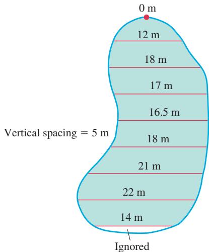
b. At what altitude does B’s parachute open?
a. At what altitude does A’s parachute open?
c. Which skydiver lands first?
- Suppose
∫ 2 − 2 𝑓 ( 𝑥 ) 𝑑 𝑥 = 4 ∫ 5 2 𝑓 ( 𝑥 ) 𝑑 𝑥 = 3 ∫ 5 − 2 𝑔 ( 𝑥 ) 𝑑 𝑥 = 2
Which, if any, of the following statements are true?
a.
c.
3. Initial value problem Show that
solves the initial value problem
(Hint:
- Proportionality Suppose that x and y are related by the equation
Show that
- Find
𝑓 ( 4 )
- Find
𝑓 ( 𝜋 / 2 )
i)
ii) The area under the curve
-
The area of the region in the
𝑥 𝑦 𝑥 𝑦 = 𝑓 ( 𝑥 ) 𝑓 ( 𝑥 ) ≥ 0 𝑥 = 1 𝑥 = 𝑏 √ 𝑏 2 + 1 − √ 2 𝑏 > 1 𝑓 ( 𝑥 ) -
Prove that
(Hint: Express the integral on the right-hand side as the difference of two integrals. Then show that both sides of the equation have the same derivative with respect to x.)
-
Finding a curve Find the equation for the curve in the
𝑥 𝑦 ( 1 , − 1 ) 𝑥 3 𝑥 2 + 2 -
Shoveling dirt You sling a shovelful of dirt up from the bottom of a hole with an initial velocity of 9.8 m/s. The dirt must rise 5.2 m above the release point to clear the edge of the hole. Is that enough speed to get the dirt out, or had you better duck?
Piecewise Continuous Functions
Although we are mainly interested in continuous functions, many functions in applications are piecewise continuous. A function
exist and are finite at every interior point of I, and the appropriate one-sided limits exist and are finite at the endpoints of I. All piecewise continuous functions are integrable. The points of discontinuity subdivide I into open and half-open subintervals on which f is continuous, and the limit criteria above guarantee that f has a continuous extension to the closure of each subinterval. To integrate a piecewise continuous function, we integrate the individual extensions and add the results. The integral of
(Figure 5.33) over
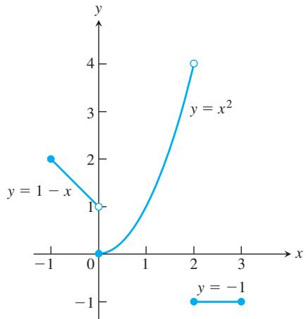
FIGURE 5.33 Piecewise continuous
functions like this are integrated piece by piece.
The Fundamental Theorem applies to piecewise continuous functions with the restriction that
Graph the functions in Exercises 11–16 and integrate them over their domains.
- Find the average value of the function graphed in the accompanying figure.
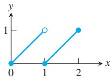
- Find the average value of the function graphed in the accompanying figure.
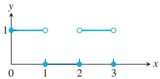
Limits
Find the limits in Exercises 19–22.
-
l i m 𝑏 → 1 − ∫ 𝑏 0 𝑑 𝑥 √ 1 − 𝑥 2 l i m 𝑥 → ∞ 1 𝑥 ∫ 𝑥 0 a r c t a n 𝑡 𝑑 𝑡 -
l i m 𝑛 → ∞ ( 1 𝑛 + 1 + 1 𝑛 + 2 + ⋯ + 1 2 𝑛 ) -
l i m 𝑛 → ∞ 1 𝑛 ( 𝑒 1 / 𝑛 + 𝑒 2 / 𝑛 + ⋯ + 𝑒 ( 𝑛 − 1 ) / 𝑛 + 𝑒 𝑛 / 𝑛 )
Defining Functions Using the Fundamental Theorem
- A function defined by an integral The graph of a function
𝑓 𝑔 ( 𝑥 ) = ∫ 𝑥 1 𝑓 ( 𝑡 ) 𝑑 𝑡
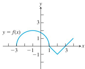
a. Find
d. Find all values of x on the open interval
e. Write an equation for the line tangent to the graph of g at x = -1.
f. Find the
g. Find the range of g.
- A differential equation Show that both of the following conditions are satisfied by
𝑦 = s i n 𝑥 + ∫ 𝜋 𝑥 c o s 2 𝑡 𝑑 𝑡 + 1
i)
ii)
Leibniz’s Rule In applications, we sometimes encounter functions defined by integrals that have variable upper limits of integration and variable lower limits of integration at the same time. We can find the derivative of such an integral by a formula called Leibniz’s Rule.
Leibniz’s Rule
If
To prove the rule, let
Differentiating both sides of this equation with respect to
Use Leibniz’s Rule to find the derivatives of the functions in Exercises 25-32.
-
𝑓 ( 𝑥 ) = ∫ 𝑥 1 / 𝑥 1 𝑡 𝑑 𝑡 -
𝑓 ( 𝑥 ) = ∫ s i n 𝑥 c o s 𝑥 1 1 − 𝑡 2 𝑑 𝑡 -
𝑔 ( 𝑦 ) = ∫ 2 √ 𝑦 √ 𝑦 s i n 𝑡 2 𝑑 𝑡 -
𝑔 ( 𝑦 ) = ∫ 𝑦 2 √ 𝑦 𝑒 𝑡 𝑡 𝑑 𝑡 -
𝑦 = ∫ 𝑥 2 𝑥 2 / 2 l n √ 𝑡 𝑑 𝑡 -
𝑦 = ∫ 3 √ 𝑥 √ 𝑥 l n 𝑡 𝑑 𝑡 -
𝑦 = ∫ l n 𝑥 0 s i n 𝑒 𝑡 𝑑 𝑡 -
𝑦 = ∫ 𝑒 2 𝑥 𝑒 4 √ 𝑥 l n 𝑡 𝑑 𝑡
Theory and Examples
- Use Leibniz’s Rule to find the value of
𝑥
-
For what x > 0 does
𝑥 ( 𝑥 𝑥 ) = ( 𝑥 𝑥 ) 𝑥 -
For the two curves
𝑦 = 2 ( l o g 2 𝑥 ) / 𝑥 𝑦 = 2 ( l o g 4 𝑥 ) / 𝑥 𝑥 𝑥 = 1 𝑥 = 𝑒
b. Find the area between the second curve and the
c. Consider the two areas obtained in parts (a) and (b). What is the ratio of the larger area to the smaller?
- a. Find
𝑑 𝑓 / 𝑑 𝑥
b. Find
c. What can you conclude about the graph of
-
Find
𝑓 ′ ( 2 ) 𝑓 ( 𝑥 ) = 𝑒 𝑔 ( 𝑥 ) 𝑔 ( 𝑥 ) = ∫ 𝑥 2 𝑡 1 + 𝑡 4 𝑑 𝑡 -
Use the accompanying figure to show that
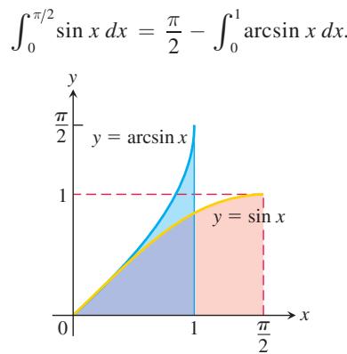
- Napier’s inequality Here are two pictorial proofs that
Explain what is going on in each case.
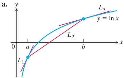
b.
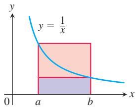
(Source: Roger B. Nelson, College Mathematics Journal, Vol. 24, No. 2, March 1993, p. 165.)
- Bound on an integral Let f be a continuously differentiable function on
[ 𝑎 , 𝑏 ] ∫ 𝑏 𝑎 𝑓 ( 𝑥 ) 𝑑 𝑥 = 0
a. If
b. Let
c. Apply the Mean Value Theorem from Section 4.2 to part (b) to prove that
where M is the absolute maximum of
Approximating Finite Sums with Integrals
In many applications of calculus, integrals are used to approximate finite sums—the reverse of the usual procedure of using finite sums to approximate integrals.
For example, let’s estimate the sum of the square roots of the first
is the limit of the upper sums
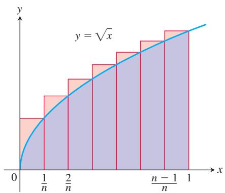
Therefore, when n is large,
The following table shows how good the approximation can be.
| n | Root sum | Relative error | |
| 10 | 22.468 | 21.082 | 1.386/22.468 ≈ 6% |
| 50 | 239.04 | 235.70 | 1.4% |
| 100 | 671.46 | 666.67 | 0.7% |
| 1000 | 21,097 | 21,082 | 0.07% |
- Evaluate
by showing that the limit is
and evaluating the integral.
- See Exercise 41. Evaluate
- Let
𝑓 ( 𝑥 )
as a definite integral.
- Use the result of Exercise 43 to evaluate
b.
What can be said about the following limits?
d.
e.
- a. Show that the area
𝐴 𝑛 𝑛 𝑟
b. Find the limit of
- Let
To calculate
and interpret
(Hint: Partition
CHAPTER 5 Technology Application Projects
Mathematica/Maple Projects
Projects can be found within MyLab Math.
-
Using Riemann Sums to Estimate Areas, Volumes, and Lengths of Curves Visualize and approximate areas and volumes in Part I.
-
Riemann Sums, Definite Integrals, and the Fundamental Theorem of Calculus Parts I, II, and III develop Riemann sums and definite integrals. Part IV continues the development of the Riemann sum and definite integral using the Fundamental Theorem to solve problems previously investigated.
• Rain Catchers, Elevators, and Rockets
Part I illustrates that the area under a curve is the same as the area of an appropriate rectangle for examples taken from the chapter. You will compute the amount of water accumulating in basins of different shapes as the basin is filled and drained.
• Motion Along a Straight Line, Part II
You will observe the shape of a graph through dramatic animated visualizations of the derivative relations among position, velocity, and acceleration. Figures in the text can be animated using this software.
- Bending of Beams
Study bent shapes of beams, determine their maximum deflections, concavity, and inflection points, and interpret the results in terms of a beam’s compression and tension.