Chapter 15: Integrals and Vector Fields
OVERVIEW In this chapter we extend the theory of integration to functions whose domains are curves and surfaces in space. The resulting line and surface integrals give powerful mathematical tools for science and engineering. Line integrals are used to find the work done by a force in moving an object along a path and to find the mass of a curved wire with variable density. Surface integrals are used to find the rate of flow of a fluid across a surface and to describe the interactions of electric and magnetic forces. We present the fundamental theorems of vector integral calculus and discuss their mathematical consequences and physical applications. The theorems of vector calculus are then shown to be generalized versions of the Fundamental Theorem of Calculus.
15.1 Line Integrals of Scalar Functions
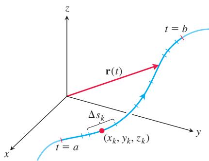
To calculate the total mass of a wire lying along a curve in space, or to find the work done by a variable force acting along such a curve, we need a more general notion of integral than was defined in Chapter 5. We need to integrate over a curve C rather than over an interval
FIGURE 15.1 The curve
Suppose that
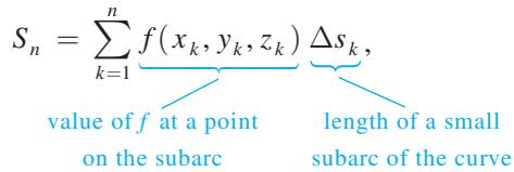
which is similar to a Riemann sum. Depending on how we partition the curve C and pick
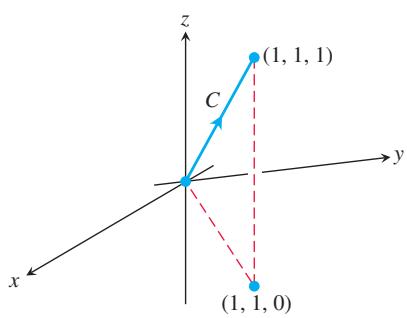
FIGURE 15.2 The integration path in Example 1.
DEFINITION If
is defined on a curve 𝑓 given parametrically by 𝐶 , then the line integral of 𝐫 ( 𝑡 ) = 𝑔 ( 𝑡 ) 𝐢 + ℎ ( 𝑡 ) 𝐣 + 𝑘 ( 𝑡 ) 𝐤 , 𝑎 ≤ 𝑡 ≤ 𝑏 over 𝑓 is 𝐶 ∫ 𝐶 𝑓 ( 𝑥 , 𝑦 , 𝑧 ) 𝑑 𝑠 = l i m 𝑛 → ∞ 𝑛 ∑ 𝑘 = 1 𝑓 ( 𝑥 𝑘 , 𝑦 𝑘 , 𝑧 𝑘 ) Δ 𝑠 𝑘 , ( 1 ) provided this limit exists.
𝑓 ( 𝐫 ( 𝑡 ) ) = 𝑓 ( 𝑔 ( 𝑡 ) , ℎ ( 𝑡 ) , 𝑘 ( 𝑡 ) ) If the curve C is smooth for
(so 𝑎 ≤ 𝑡 ≤ 𝑏 is continuous and never 0) and the function f is continuous on C, then the limit in Equation (1) can be shown to exist. We can then apply the Fundamental Theorem of Calculus to differentiate the arc length equation, 𝑣 = 𝑑 𝑟 / 𝑑 𝑡 𝑠 ( 𝑡 ) = ∫ 𝑡 𝑎 | 𝐯 ( 𝜏 ) | 𝑑 𝜏 , E q . ( 3 ) o f S e c t i o n 1 2 . 3 w i t h 𝑡 0 = 𝑎 𝑑 𝑠 𝑑 𝑡 = | 𝐯 | = √ ( 𝑑 𝑥 𝑑 𝑡 ) 2 + ( 𝑑 𝑦 𝑑 𝑡 ) 2 + ( 𝑑 𝑧 𝑑 𝑡 ) 2 to express ds in Equation (1) as
and evaluate the integral of f over C as 𝑑 𝑠 = | 𝐯 ( 𝑡 ) | 𝑑 𝑡 ∫ 𝐶 𝑓 ( 𝑥 , 𝑦 , 𝑧 ) 𝑑 𝑠 = ∫ 𝑏 𝑎 𝑓 ( 𝑔 ( 𝑡 ) , ℎ ( 𝑡 ) , 𝑘 ( 𝑡 ) ) | 𝐯 ( 𝑡 ) | 𝑑 𝑡 . ( 2 )
The integral on the right side of Equation (2) is just an ordinary definite integral, as defined in Chapter 5, where we are integrating with respect to the parameter t. The formula evaluates the line integral on the left side correctly no matter what smooth parametrization is used. Note that the parameter t defines a direction along the path. The starting point on C is the position
How to Evaluate a Line Integral
To integrate a continuous function
- Find a smooth parametrization of C,
- Evaluate the integral as
If f has the constant value 1, then the integral of f over C gives the length of C from t = a to t = b. We also write
EXAMPLE 1 Integrate
Solution Since any choice of parametrization will give the same answer, we choose the simplest parametrization we can think of:
The components have continuous first derivatives, and
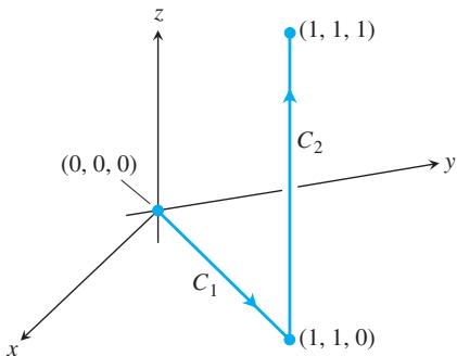
FIGURE 15.3 The path of integration in Example 2.
Additivity
Line integrals have the useful property that if a piecewise smooth curve C is made by joining a finite number of smooth curves
EXAMPLE 2 Figure 15.3 shows another path from the origin to
Solution We choose the simplest parametrizations for
With these parametrizations we find that
Notice three things about the integrations in Examples 1 and 2. First, as soon as the components of the appropriate curve were substituted into the formula for f, the integration became a standard integration with respect to t. Second, the integral of f over
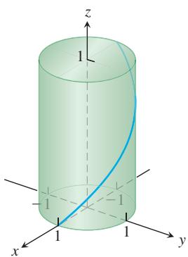
FIGURE 15.4 A line integral is taken over a curve such as this helix from Example 3.
The value of a line integral along a path joining two points can change if you change the path between them.
EXAMPLE 3 Find the line integral of
Solution For the helix (Figure 15.4) we find
The line integral is given by
Mass and Moment Calculations
We treat coil springs and wires as masses distributed along smooth curves in space. The distribution is described by a continuous density function
(See Section 12.3.) The spring’s or wire’s mass, center of mass, and moments are then calculated using the formulas in Table 15.1, with the integrations in terms of the parameter
These formulas also apply to thin rods, and their derivations are similar to those in Section 6.6. Notice how similar the formulas are to those in Tables 15.1 and 15.2 for double and triple integrals. The double integrals for planar regions, and the triple integrals for solids, become line integrals for coil springs, wires, and thin rods.
Notice that the element of mass dm is equal to
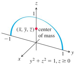
FIGURE 15.5 Example 4 shows how to find the center of mass of a circular arch of variable density.
EXAMPLE 4 A slender metal arch, denser at the bottom than at the top, lies along the semicircle
Solution We know that
TABLE 15.1 Mass and moment formulas for coil springs, wires, and thin rods lying along a smooth curve C in space
Mass:
First moments about the coordinate planes:
Coordinates of the center of mass:
Moments of inertia about axes and other lines:
For this parametrization,
so ds = |v| dt = dt.
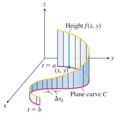
FIGURE 15.6 The line integral
The formulas in Table 15.1 then give
With
Line Integrals in the Plane
Line integrals for curves in the plane have a natural geometric interpretation. If C is a smooth curve in the xy-plane parametrized by
h.
f.
where
EXERCISES 15.1
Graphs of Vector Equations
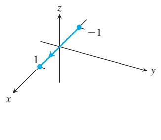
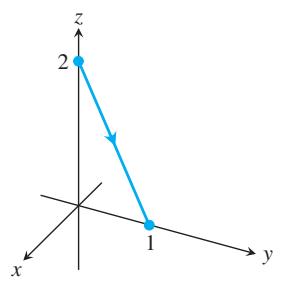
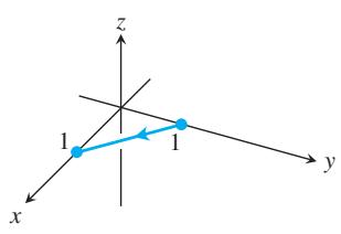
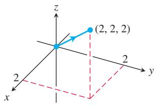
Match the vector equations in Exercises 1–8 with the graphs (a)–(h) given here.
a.
b.
c.
d.
e.
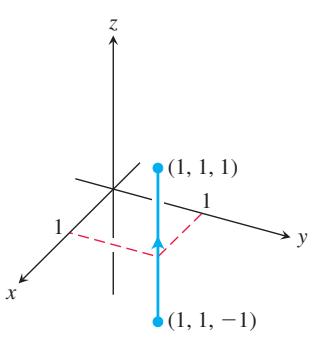
g.
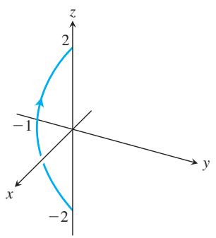
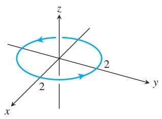
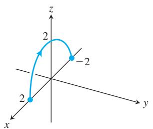
Evaluating Line Integrals over Space Curves
-
Evaluate
∫ 𝐶 ( 𝑥 + 𝑦 ) 𝑑 𝑠 𝐶 𝑥 = 𝑡 𝑦 = ( 1 − 𝑡 ) 𝑧 = 0 ( 0 , 1 , 0 ) ( 1 , 0 , 0 ) -
Evaluate
∫ 𝐶 ( 𝑥 − 𝑦 + 𝑧 − 2 ) 𝑑 𝑠 𝐶 𝑥 = 𝑡 𝑦 = ( 1 − 𝑡 ) 𝑧 = 1 ( 0 , 1 , 1 ) ( 1 , 0 , 1 ) -
Evaluate
∫ 𝐶 ( 𝑥 𝑦 + 𝑦 + 𝑧 ) 𝑑 𝑠 𝐫 ( 𝑡 ) = 2 𝑡 𝐢 + 𝑡 𝐣 + ( 2 − 2 𝑡 ) 𝐤 , 0 ≤ 𝑡 ≤ 1 -
Evaluate
∫ 𝐶 √ 𝑥 2 + 𝑦 2 𝑑 𝑠 𝐫 ( 𝑡 ) = ( 4 c o s 𝑡 ) 𝐢 + ( 4 s i n 𝑡 ) 𝐣 + 3 𝑡 𝐤 , − 2 𝜋 ≤ 𝑡 ≤ 2 𝜋 -
Find the line integral of
𝑓 ( 𝑥 , 𝑦 , 𝑧 ) = 𝑥 + 𝑦 + 𝑧 ( 1 , 2 , 3 ) ( 0 , − 1 , 1 ) -
Find the line integral of
𝑓 ( 𝑥 , 𝑦 , 𝑧 ) = √ 3 / ( 𝑥 2 + 𝑦 2 + 𝑧 2 ) 𝐫 ( 𝑡 ) = 𝑡 𝐢 + 𝑡 𝐣 + 𝑡 𝐤 , 1 ≤ 𝑡 < ∞ -
Integrate
𝑓 ( 𝑥 , 𝑦 , 𝑧 ) = 𝑥 + √ 𝑦 − 𝑧 2 𝐶 1 𝐶 2
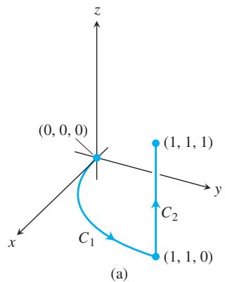
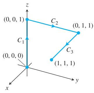
(b)
The paths of integration for Exercises 15 and 15.
- Integrate
𝑓 ( 𝑥 , 𝑦 , 𝑧 ) = 𝑥 + √ 𝑦 − 𝑧 2 𝐶 1 𝐶 2 𝐶 3 ( 0 , 0 , 0 ) ( 1 , 1 , 1 )
-
Integrate
𝑓 ( 𝑥 , 𝑦 , 𝑧 ) = ( 𝑥 + 𝑦 + 𝑧 ) / ( 𝑥 2 + 𝑦 2 + 𝑧 2 ) 𝐫 ( 𝑡 ) = 𝑡 𝐢 + 𝑡 𝐣 + 𝑡 𝐤 , 0 < 𝑎 ≤ 𝑡 ≤ 𝑏 -
Integrate
𝑓 ( 𝑥 , 𝑦 , 𝑧 ) = − √ 𝑥 2 + 𝑧 2
Line Integrals over Plane Curves
-
Evaluate
∫ 𝐶 𝑥 𝑑 𝑠 𝐶 𝑥 = 𝑡 𝑦 = 𝑡 / 2 ( 0 , 0 ) ( 4 , 2 ) 𝑥 = 𝑡 𝑦 = 𝑡 2 ( 0 , 0 ) ( 2 , 4 ) -
Evaluate
∫ 𝐶 √ 𝑥 + 2 𝑦 𝑑 𝑠 𝐶
a. the straight-line segment
b.
-
Find the line integral of
𝑓 ( 𝑥 , 𝑦 ) = 𝑦 𝑒 𝑥 2 𝐫 ( 𝑡 ) = 4 𝑡 𝑖 − 3 𝑡 𝐣 , − 1 ≤ 𝑡 ≤ 2 . -
Find the line integral of
𝑓 ( 𝑥 , 𝑦 ) = 𝑥 − 𝑦 + 3 𝐫 ( 𝑡 ) = ( c o s 𝑡 ) 𝐢 + ( s i n 𝑡 ) 𝐣 , 0 ≤ 𝑡 ≤ 2 𝜋 . -
Evaluate
∫ 𝐶 𝑥 2 𝑦 4 / 3 𝑑 𝑠 𝐶 𝑥 = 𝑡 2 𝑦 = 𝑡 3 1 ≤ 𝑡 ≤ 2 -
Find the line integral of
𝑓 ( 𝑥 , 𝑦 ) = √ 𝑦 / 𝑥 𝐫 ( 𝑡 ) = 𝑡 3 𝐢 + 𝑡 4 𝐣 , 1 / 2 ≤ 𝑡 ≤ 1 -
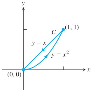
Evaluate
∫ 𝐶 ( 𝑥 + √ 𝑦 ) 𝑑 𝑠 𝐶
- Evaluate
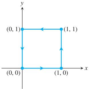
∫ 𝐶 1 𝑥 2 + 𝑦 2 + 1 𝑑 𝑠 𝐶
In Exercises 27–30, integrate f over the given curve.
-
𝑓 ( 𝑥 , 𝑦 ) = 𝑥 3 / 𝑦 𝐶 : 𝑦 = 𝑥 2 / 2 0 ≤ 𝑥 ≤ 2 -
𝑓 ( 𝑥 , 𝑦 ) = ( 𝑥 + 𝑦 2 ) / √ 1 + 𝑥 2 𝑦 = 𝑥 2 / 2 ( 1 , 1 / 2 ) ( 0 , 0 ) -
𝑓 ( 𝑥 , 𝑦 ) = 𝑥 + 𝑦 𝐶 : 𝑥 2 + 𝑦 2 = 4 -
𝑓 ( 𝑥 , 𝑦 ) = 𝑥 2 − 𝑦 𝐶 : 𝑥 2 + 𝑦 2 = 4 ( √ 2 , √ 2 ) -
Find the area of one side of the “winding wall” standing perpendicularly on the curve
𝑦 = 𝑥 2 0 ≤ 𝑥 ≤ 2 𝑓 ( 𝑥 , 𝑦 ) = 𝑥 + √ 𝑦 -
Find the area of one side of the “wall” standing perpendicularly on the curve
2 𝑥 + 3 𝑦 = 6 0 ≤ 𝑥 ≤ 6 𝑓 ( 𝑥 , 𝑦 ) = 4 + 3 𝑥 + 2 𝑦
Masses and Moments
-
Mass of a wire Find the mass of a wire that lies along the curve
𝐫 ( 𝑡 ) = ( 𝑡 2 − 1 ) 𝐣 + 2 𝑡 𝐤 , 0 ≤ 𝑡 ≤ 1 𝛿 = ( 3 / 2 ) 𝑡 -
Center of mass of a curved wire A wire of density
𝛿 ( 𝑥 , 𝑦 , 𝑧 ) = 1 5 √ 𝑦 + 2 𝐫 ( 𝑡 ) = ( 𝑡 2 − 1 ) 𝐣 + 2 𝑡 𝑘 , − 1 ≤ 𝑡 ≤ 1 -
Mass of wire with variable density Find the mass of a thin wire lying along the curve
𝐫 ( 𝑡 ) = √ 2 𝑡 𝐢 + √ 2 𝑡 𝐣 + ( 4 − 𝑡 2 ) 𝐤 0 ≤ 𝑡 ≤ 1 𝛿 = 3 𝑡 𝛿 = 1 -
Center of mass of wire with variable density Find the center of mass of a thin wire lying along the curve
𝐫 ( 𝑡 ) = 𝑡 𝐢 + 2 𝑡 𝐣 + ( 2 / 3 ) 𝑡 3 / 2 𝐤 , 0 ≤ 𝑡 ≤ 2 𝛿 = 3 √ 5 + 𝑡 -
Moment of inertia of wire hoop A circular wire hoop of constant density
𝛿 𝑥 2 + 𝑦 2 = 𝑎 2 𝑥 𝑦 𝑧 -
Inertia of a slender rod A slender rod of constant density lies along the line segment
𝐫 ( 𝑡 ) = 𝑡 𝐣 + ( 2 − 2 𝑡 ) 𝐤 , 0 ≤ 𝑡 ≤ 1 -
Two springs of constant density lies along the helix A spring of constant density
𝛿
a. Find
b. Suppose that you have another spring of constant density
- Wire of constant density A wire of constant density
𝛿 = 1
Find
-
The arch in Example 4 Find
𝐼 𝑥 -
Center of mass and moments of inertia for wire with variable density Find the center of mass and the moments of inertia about the coordinate axes of a thin wire lying along the curve
if the density is
COMPUTER EXPLORATIONS
In Exercises 43–46, use a CAS to perform the following steps to evaluate the line integrals.
a. Find
b. Express the integrand
c. Evaluate
-
𝑓 ( 𝑥 , 𝑦 , 𝑧 ) = √ 1 + 3 0 𝑥 2 + 1 0 𝑦 ; 𝐫 ( 𝑡 ) = 𝑡 𝐢 + 𝑡 2 𝐣 + 3 𝑡 2 𝐤 , 0 ≤ 𝑡 ≤ 2 -
𝑓 ( 𝑥 , 𝑦 , 𝑧 ) = √ 1 + 𝑥 3 + 5 𝑦 3 𝐫 ( 𝑡 ) = 𝑡 𝐢 + 1 3 𝑡 2 𝐣 + √ 𝑡 𝐤 , 0 ≤ 𝑡 ≤ 2 -
𝑓 ( 𝑥 , 𝑦 , 𝑧 ) = 𝑥 √ 𝑦 − 3 𝑧 2 ; 𝐫 ( 𝑡 ) = ( c o s 2 𝑡 ) 𝐢 + ( s i n 2 𝑡 ) 𝐣 + 5 𝑡 𝐤 , 0 ≤ 𝑡 ≤ 2 𝜋 -
𝑓 ( 𝑥 , 𝑦 , 𝑧 ) = ( 1 + 9 4 𝑧 1 / 3 ) 1 / 4 ;
15.2 Vector Fields and Line Integrals: Work, Circulation, and Flux
Gravitational and electric forces have both a direction and a magnitude. They are represented by a vector at each point in their domain, producing a vector field. In this section we show how to compute the work done in moving an object through such a field by using a line integral involving the vector field. We also discuss velocity fields, such as the vector field representing the velocity of a flowing fluid in its domain. A line integral can be used to find the rate at which the fluid flows along or across a curve within the domain.
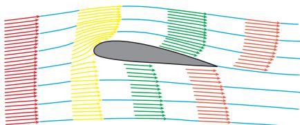
FIGURE 15.7 Velocity vectors of a flow around an airfoil.
Vector Fields
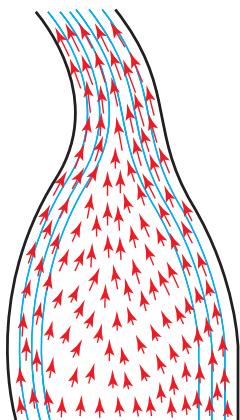
FIGURE 15.8 Streamlines in a contracting channel. The water speeds up as the channel narrows, and the velocity vectors increase in length.
Suppose a region in the plane or in space is occupied by a moving fluid, such as air or water. The fluid is made up of a large number of particles, and at any instant of time, a particle has a velocity v. At different points of the region at a given (same) time, these velocities can vary. We can think of a velocity vector being attached to each point of the fluid, representing the velocity of a particle at that point. Such a fluid flow is an example of a vector field. Figure 15.7 shows a velocity vector field obtained from air flowing around an airfoil in a wind tunnel. Figure 15.8 shows a vector field of velocity vectors along the streamlines of water moving through a contracting channel. Vector fields are also associated with forces such as gravitational attraction (Figure 15.9) and with magnetic fields and electric fields. There are purely mathematical fields as well.
Generally, a vector field is a function that assigns a vector to each point in its domain. A vector field on a three-dimensional domain in space might have a formula like
The vector field is continuous if the component functions M, N, and P are continuous; it is differentiable if each of the component functions is differentiable. The formula for a field of two-dimensional vectors could look like
We encountered another type of vector field in Chapter 12. The tangent vectors T and normal vectors N for a curve in space both form vector fields along the curve. Along a curve
If we attach the gradient vector
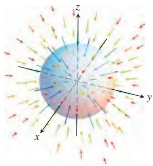
FIGURE 15.9 Vectors in a gravitational field point toward the center of mass that gives the source of the field.
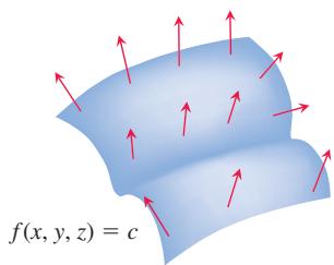
FIGURE 15.11 The field of gradient vectors
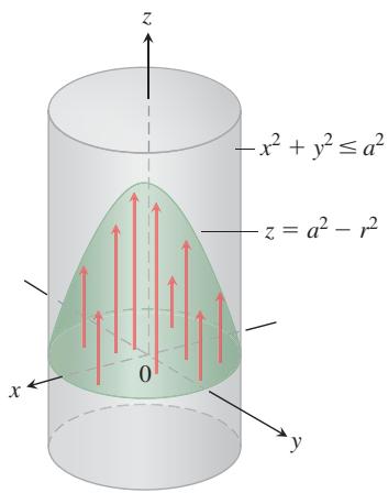
FIGURE 15.14 The flow of fluid in a long cylindrical pipe. The vectors
defined on a region in space. These and other fields are illustrated in Figures 15.7–15.16. To sketch the fields, we picked a representative selection of domain points and drew the vectors attached to them. The arrows are drawn with their tails, not their heads, attached to the points where the vector functions are evaluated.
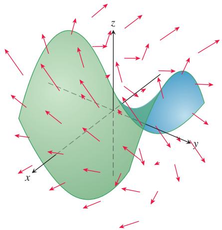
FIGURE 15.10 A surface might represent a filter (or a net or a parachute) in a vector field representing water or wind flow velocity vectors. The arrows show the direction of fluid flow, and their lengths indicate speed.
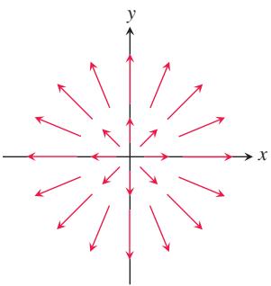
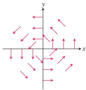
FIGURE 15.12 The radial field
FIGURE 15.13 A “spin” field of rotating unit vectors
in the plane. The field is not defined at the origin.
Gradient Fields
The gradient vector of a differentiable scalar-valued function at a point gives the direction of greatest increase of the function. An important type of vector field is formed by all the gradient vectors of the function (see Section 13.5). We define the gradient field of a differentiable function
At each point
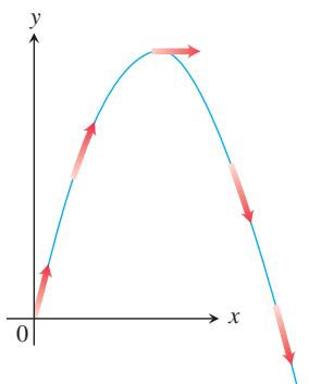
FIGURE 15.15 The velocity vectors
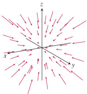
FIGURE 15.17 The vectors in a temperature gradient field point in the direction of greatest increase in temperature. In this case they are pointing toward the origin.
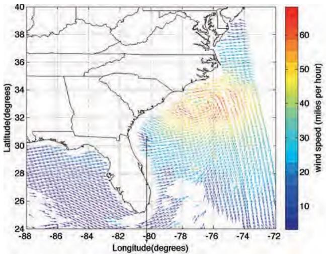
FIGURE 15.16 Data from NASA’s QuikSCAT satellite were used to create this representation of wind speed and wind direction in Hurricane Irene approximately six hours before it made landfall in North Carolina on August 27, 2011. The arrows show wind direction, and speed is indicated by color (rather than length). The maximum wind speeds (over
In many physical applications, f represents a potential energy, and the gradient vector field indicates the corresponding force. In such situations, f is often taken to be negative, so that the force gives the direction of decreasing potential energy.
EXAMPLE 1 Suppose that a material is heated, that the resulting temperature T at each point
and that
Solution The gradient field F is the field
Line Integrals of Vector Fields
In Section 15.1 we defined the line integral of a scalar function
Assume that the vector field
so we are led to the following definition.
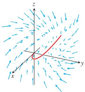
FIGURE 15.18 A curve (in red) winds through a vector field as in Example 2. The line integral is determined by the vectors that lie along the curve.
DEFINITION Let F be a vector field with continuous components defined along a smooth curve C parametrized by
, 𝐫 ( 𝑡 ) . Then the line integral of F along C is 𝑎 ≤ 𝑡 ≤ 𝑏 ∫ 𝐶 𝐅 ⋅ 𝐓 𝑑 𝑠 = ∫ 𝐶 ( 𝐅 ⋅ 𝑑 𝐫 𝑑 𝑠 ) 𝑑 𝑠 = ∫ 𝐶 𝐅 ⋅ 𝑑 𝐫 . ( 1 )
We evaluate line integrals of vector fields in a way similar to the way we evaluate line integrals of scalar functions (Section 15.1). The vector field may also be defined on points not meeting the curve, but only the vectors along the curve play a role in the line integral. See Figure 15.18.
Evaluating the Line Integral of F = M i + N j + P k Along C: r(t) = g(t)i + h(t)j + k(t)k
-
Express the vector field F along the parametrized curve C as
𝐅 ( 𝐫 ( 𝑡 ) ) 𝑥 = 𝑔 ( 𝑡 ) 𝑦 = ℎ ( 𝑡 ) 𝑧 = 𝑘 ( 𝑡 ) 𝑀 ( 𝑥 , 𝑦 , 𝑧 ) 𝑁 ( 𝑥 , 𝑦 , 𝑧 ) 𝑃 ( 𝑥 , 𝑦 , 𝑧 ) -
Find the derivative (velocity) vector dr/dt.
-
Evaluate the line integral with respect to the parameter
𝑡 𝑎 ≤ 𝑡 ≤ 𝑏
EXAMPLE 2 Evaluate
Solution We have
and
Thus,
Line Integrals with Respect to dx, dy, or dz
When analyzing forces or flows, it is often useful to consider each component direction separately. For example, when analyzing the effect of a gravitational force, we might want to consider motion and forces in the vertical direction, while ignoring horizontal motions. Or we might be interested only in the force exerted horizontally by water pushing against the face of a dam or in wind affecting the course of a plane. In such situations we want to evaluate a line integral of a scalar function with respect to only one of the coordinates, such as
Line Integral Notation
To evaluate these integrals, we parametrize C as
is a short way of expressing the sum of three line integrals, one for each coordinate direction:
As in the definition of the line integral of F along C, we define
The commonly occurring expression
In the same way, by defining
It often happens that these line integrals occur in combination, and we abbreviate the notation by writing
EXAMPLE 3 Evaluate the line integral
Solution We express everything in terms of the parameter t, so
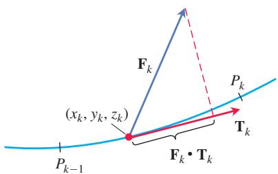
FIGURE 15.19 The work done along the subarc shown here is approximately
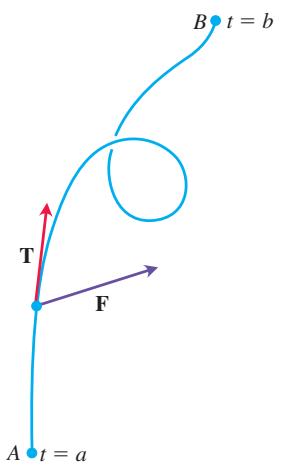
FIGURE 15.20 The work done by a force F is the line integral of the scalar component
Work Done by a Force over a Curve in Space
Suppose that the vector field
represents a smooth curve C in the region. The formula for the work done by the force in moving an object along the curve is motivated by the same kind of reasoning we used in Chapter 6 to derive the ordinary single integral for the work done by a continuous force of magnitude
We divide C into n subarcs
For any subdivision of C into n subarcs, and for any choice of the points
This is the line integral of
DEFINITION Let C be a smooth curve parametrized by
, 𝐫 ( 𝑡 ) , and let F be a continuous force field over a region containing C. Then the work done in moving an object from the point 𝑎 ≤ 𝑡 ≤ 𝑏 to the point 𝐴 = 𝐫 ( 𝑎 ) along C is 𝐵 = 𝐫 ( 𝑏 ) 𝑊 = ∫ 𝐶 𝐅 ⋅ 𝐓 𝑑 𝑠 = ∫ 𝑏 𝑎 𝐅 ( 𝐫 ( 𝑡 ) ) ⋅ 𝑑 𝐫 𝑑 𝑡 𝑑 𝑡 . ( 6 )
The sign of the number we calculate with this integral depends on the direction in which the curve is traversed. If we reverse the direction of motion, then we reverse the direction of T in Figure 15.20 and change the sign of
Using the notations we have presented, we can express the work integral in a variety of ways, depending upon what seems most suitable or convenient for a particular discussion. Table 15.2 shows five ways we can write the work integral in Equation (6). In the table, the field components M, N, and P are functions of the intermediate variables x, y, and z, which in turn are functions of the independent variable t along the curve C in the vector field. So along the curve,
TABLE 15.2 Different ways to write the work integral for F = M i + N j + P k over the curve C: r(t) = g(t)i + h(t)j + k(t)k, a ≤ t ≤ b
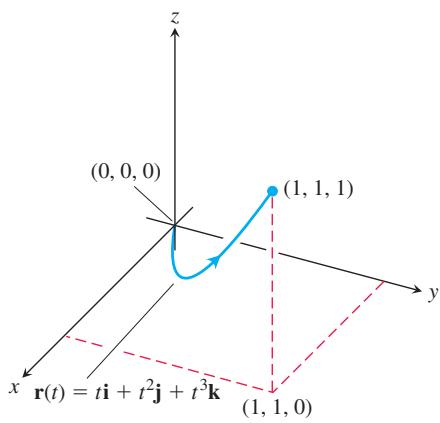
FIGURE 15.21 The curve in Example 4.
EXAMPLE 4 Find the work done by the force field
Solution First we evaluate F on the curve
Then we find
Finally, we find
Thus
EXAMPLE 5 Find the work done by the force field
Solution We begin by writing F along C as a function of t:
Next we compute dr/dt:
We then calculate the dot product:
The work done is the line integral
Flow Integrals and Circulation for Velocity Fields
Suppose that
DEFINITION If
parametrizes a smooth curve C in the domain of a continuous velocity field F, then the flow along the curve from 𝐫 ( 𝑡 ) to 𝐴 = 𝐫 ( 𝑎 ) is 𝐵 = 𝐫 ( 𝑏 ) F l o w = ∫ 𝐶 𝐅 ⋅ 𝐓 𝑑 𝑠 . ( 7 )
The integral is called a flow integral. If the curve starts and ends at the same point, so that A = B, the flow is called the circulation around the curve.
The direction we travel along C matters. If we reverse the direction, then T is replaced by -T and the sign of the integral changes. We evaluate flow integrals the same way we evaluate work integrals.
EXAMPLE 6 A fluid’s velocity field is
Solution We evaluate F on the curve
and then find
The dot product of
Finally, we integrate
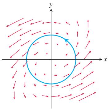
FIGURE 15.22 The vector field F and curve
Simple, not closed
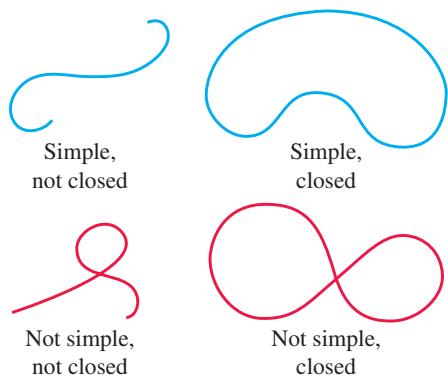
FIGURE 15.23 Distinguishing between curves that are simple and curves that are closed. Closed curves are also called loops.
EXAMPLE 7 Find the circulation of the field
Then
Solution On the circle,
gives
As Figure 15.22 suggests, a fluid with this velocity field is circulating counterclockwise around the circle. The circle is also traversed counterclockwise as t increases from 0 to
Flux Across a Simple Closed Plane Curve
A curve in the xy-plane is simple if it does not cross itself (Figure 15.23). When a curve starts and ends at the same point, it is a closed curve or loop. To find the rate at which a fluid is entering or leaving a region enclosed by a smooth simple closed curve C in the xy-plane, we calculate the line integral over C of
DEFINITION If C is a smooth simple closed curve in the domain of a continuous vector field
in the plane, and if n is the outward-pointing unit normal vector on C, the flux of F across C is 𝐅 = 𝑀 ( 𝑥 , 𝑦 ) 𝐢 + 𝑁 ( 𝑥 , 𝑦 ) 𝐣 F l u x o f 𝐅 a c r o s s 𝐶 = ∫ 𝐶 𝐅 ⋅ 𝐧 𝑑 𝑠 . ( 8 )
Notice the difference between flux and circulation. The flux of F across C is the line integral with respect to arc length of
To evaluate the integral for flux in Equation (8), we begin with a smooth parametrization
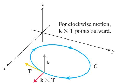
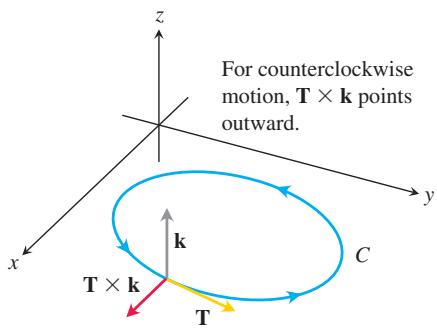
FIGURE 15.24 To find an outward unit normal vector for a smooth simple curve C in the xy-plane that is traversed counterclockwise as t increases, we take
that traces the curve
In terms of components,
If
Hence,
We put a directed circle
Calculating Flux Across a Smooth Closed Plane Curve
The integral can be evaluated from any smooth parametrization
EXAMPLE 8 Find the flux of
Solution The parametrization
we find
The flux of
Exercises 15.2
Vector Fields
Find the gradient fields of the functions in Exercises 1–4.
-
𝑔 ( 𝑥 , 𝑦 , 𝑧 ) = 𝑒 𝑧 − l n ( 𝑥 2 + 𝑦 2 ) -
𝑔 ( 𝑥 , 𝑦 , 𝑧 ) = 𝑥 𝑦 + 𝑦 𝑧 + 𝑥 𝑧 -
Give a formula
𝐅 = 𝑀 ( 𝑥 , 𝑦 ) 𝐢 + 𝑁 ( 𝑥 , 𝑦 ) 𝐣 𝐅 ( 𝑥 , 𝑦 ) ( 0 , 0 ) -
Give a formula
𝐅 = 𝑀 ( 𝑥 , 𝑦 ) 𝐢 + 𝑁 ( 𝑥 , 𝑦 ) 𝐣 𝐹 = 0 ( 0 , 0 ) ( 𝑎 , 𝑏 ) 𝑥 2 + 𝑦 2 = 𝑎 2 + 𝑏 2 | 𝐹 | = √ 𝑎 2 + 𝑏 2
Line Integrals of Vector Fields
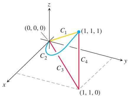
In Exercises 7–12, find the line integrals of F from
a. The straight-line path
b. The curved path
c. The path
-
𝐅 = 3 𝑦 𝐢 + 2 𝑥 𝐣 + 4 𝑧 𝐤 -
𝐅 = [ 1 / ( 𝑥 2 + 1 ) ] 𝐣 -
𝐅 = √ 𝑧 𝐢 − 2 𝑥 𝐣 + √ 𝑦 𝐤 -
𝐅 = 𝑥 𝑦 𝐢 + 𝑦 𝑧 𝐣 + 𝑥 𝑧 𝐤 -
𝐅 = ( 3 𝑥 2 − 3 𝑥 ) 𝐢 + 3 𝑧 𝐣 + 𝐤 -
𝐅 = ( 𝑦 + 𝑧 ) 𝐢 + ( 𝑧 + 𝑥 ) 𝐣 + ( 𝑥 + 𝑦 ) 𝐤
Line Integrals with Respect to
In Exercises 13–16, find the line integrals along the given path C.
-
∫ 𝐶 ( 𝑥 − 𝑦 ) 𝑑 𝑥 𝐶 : 𝑥 = 𝑡 𝑦 = 2 𝑡 + 1 0 ≤ 𝑡 ≤ 3 -
∫ 𝐶 𝑥 𝑦 𝑑 𝑦 𝐶 : 𝑥 = 𝑡 , 𝑦 = 𝑡 2 1 ≤ 𝑡 ≤ 2 -
∫ 𝐶 ( 𝑥 2 + 𝑦 2 ) 𝑑 𝑦
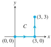
∫ 𝐶 √ 𝑥 + 𝑦 𝑑 𝑥
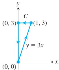
- Along the curve
𝐫 ( 𝑡 ) = 𝑡 𝐢 − 𝐣 + 𝑡 2 𝐤 0 ≤ 𝑡 ≤ 1
a.
c.
- Along the curve
𝐫 ( 𝑡 ) = ( c o s 𝑡 ) 𝐢 + ( s i n 𝑡 ) 𝐣 − ( c o s 𝑡 ) 𝐤 0 ≤ 𝑡 ≤ 𝜋
b.
Work
In Exercises 19–22, find the work done by F over the curve in the direction of increasing t.
𝐅 = 𝑥 𝑦 𝐢 + 𝑦 𝐣 − 𝑦 𝑧 𝐤
a.
Line Integrals in the Plane
-
Evaluate
∫ 𝐶 𝑥 𝑦 𝑑 𝑥 + ( 𝑥 + 𝑦 ) 𝑑 𝑦 𝑦 = 𝑥 2 ( − 1 , 1 ) ( 2 , 4 ) -
Evaluate
∫ 𝐶 ( 𝑥 − 𝑦 ) 𝑑 𝑥 + ( 𝑥 + 𝑦 ) 𝑑 𝑦 ( 0 , 0 ) , ( 1 , 0 ) ( 0 , 1 ) -
Evaluate
∫ 𝐶 𝐅 ⋅ 𝐓 𝑑 𝑠 𝐅 = 𝑥 2 𝐢 − 𝑦 𝐣 𝑥 = 𝑦 2 -
Evaluate
∫ 𝐶 𝐹 ⋅ 𝑑 𝑟 𝐹 = 𝑦 𝑖 − 𝑥 𝑗 𝑥 2 + 𝑦 2 = 1
Work, Circulation, and Flux in the Plane
-
Work Find the work done by the force
𝐅 = 𝑥 𝑦 𝐢 + ( 𝑦 − 𝑥 ) 𝐣 -
Work Find the work done by the gradient of
𝑓 ( 𝑥 , 𝑦 ) = ( 𝑥 + 𝑦 ) 2 𝑥 2 + 𝑦 2 = 4 -
Circulation and flux Find the circulation and flux of the fields
around and across each of the following curves.
a. The circle
b. The ellipse
- Flux across a circle Find the flux of the fields
across the circle
In Exercises 31–34, find the circulation and flux of the field F around and across the closed semicircular path that consists of the semicircular arch
𝐅 = 𝑥 𝐢 + 𝑦 𝐣
- Flow integrals Find the flow of the velocity field
𝐅 = ( 𝑥 + 𝑦 ) 𝐢 − ( 𝑥 2 + 𝑦 2 ) 𝐣 ( 1 , 0 ) ( − 1 , 0 )
a. The upper half of the circle
b. The line segment from
c. The line segment from
-
Flux across a triangle Find the flux of the field
𝐅 ( 1 , 0 ) ( 0 , 1 ) ( − 1 , 0 ) -
The flow of a gas with a density of
𝛿 = 0 . 0 0 1 𝑘 𝑔 / 𝑚 2 𝐫 ( 𝑡 ) = ( − s i n 𝑡 ) 𝐢 + ( c o s 𝑡 ) 𝐣 , 0 ≤ 𝑡 ≤ 2 𝜋 𝐹 = 𝛿 𝑣 𝑣 = 𝑥 𝑖 + 𝑦 2 𝑗 𝐫 ( 𝑡 ) -
The flow of a gas with a density of
𝛿 = 0 . 3 𝑘 𝑔 / 𝑚 2 𝐫 ( 𝑡 ) = ( c o s 𝑡 ) 𝐢 + ( s i n 𝑡 ) 𝐣 , 0 ≤ 𝑡 ≤ 2 𝜋 𝐹 = 𝛿 𝑣 𝑣 = 𝑥 2 𝑖 − 𝑦 𝑗 𝐫 ( 𝑡 ) -
Find the flow of the velocity field
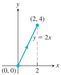
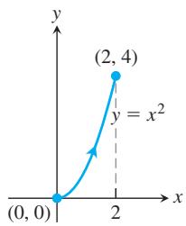
𝐹 = 𝑦 2 𝑖 + 2 𝑥 𝑦 𝑗 ( 0 , 0 ) ( 2 , 4 )
b.
c. Use any path from
- Find the circulation of the field
𝐅 = 𝑦 𝐢 + ( 𝑥 + 2 𝑦 ) 𝐣
a.
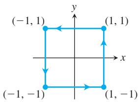
b.
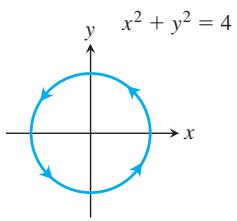
c. Use any closed path different from parts (a) and (b).
-
Find the work done by the force
𝐹 = 𝑦 2 𝑖 + 𝑥 3 𝑗 𝐫 ( 𝑡 ) = 2 𝑡 𝑖 + 𝑡 2 𝑗 0 ≤ 𝑡 ≤ 2 -
Find the work done by the force
𝐅 = 𝑒 𝑦 𝐢 + ( l n 𝑥 ) 𝐣 + 3 𝑧 𝐤 𝐫 ( 𝑡 ) = 𝑒 𝑡 𝐢 + ( l n 𝑡 ) 𝐣 + 𝑡 2 𝐤 , 1 ≤ 𝑡 ≤ 𝑒 -
Find the flow of the velocity field
𝐹 = 𝑥 𝑦 + 1 𝑖 + 𝑦 𝑥 + 1 𝑗 𝐫 ( 𝑡 ) = 𝑡 2 𝐢 + 𝑡 𝐣 , 0 ≤ 𝑡 ≤ 1 -
Find the flow of the velocity field
𝐅 = ( 𝑦 + 𝑧 ) 𝐢 + 𝑥 𝐣 − 𝑦 𝐤 𝐫 ( 𝑡 ) = 𝑒 𝑡 𝐢 − 𝑒 2 𝑡 𝐣 + 𝑒 − 𝑡 𝐤 , 0 ≤ 𝑡 ≤ l n 2 -
Salt water with a density of
𝛿 = 0 . 2 5 𝑔 / 𝑐 𝑚 2 𝐫 ( 𝑡 ) = √ 𝑡 𝑖 + 𝑡 𝐣 , 0 ≤ 𝑡 ≤ 4 𝐹 = 𝛿 𝑣 𝑣 = 𝑥 𝑦 𝐢 + ( 𝑦 − 𝑥 ) 𝐣 𝐫 ( 𝑡 ) -
Propyl alcohol with a density of
𝛿 = 0 . 2 𝑔 / 𝑐 𝑚 2 𝐫 ( 𝑡 ) = ( s i n 𝑡 ) 𝐢 − ( c o s 𝑡 ) 𝐣 , 0 ≤ 𝑡 ≤ 2 𝜋 𝐹 = 𝛿 𝑣 𝐯 = ( 𝑥 − 𝑦 ) 𝐢 + 𝑥 2 𝐣 𝐫 ( 𝑡 )
Vector Fields in the Plane
- Spin field Draw the spin field
(see Figure 15.13) along with its horizontal and vertical components at a representative assortment of points on the circle
- Radial field Draw the radial field
(see Figure 15.12) along with its horizontal and vertical components at a representative assortment of points on the circle
- A field of tangent vectors
a. Find a field
b. How is G related to the spin field F in Figure 15.13?
- A field of tangent vectors
a. Find a field
b. How is
-
Unit vectors pointing toward the origin Find a field
𝐅 = 𝑀 ( 𝑥 , 𝑦 ) 𝐢 + 𝑁 ( 𝑥 , 𝑦 ) 𝐣 ( 𝑥 , 𝑦 ) ≠ ( 0 , 0 ) ( 0 , 0 ) -
Two “central” fields Find a field
𝐅 = 𝑀 ( 𝑥 , 𝑦 ) 𝐢 + 𝑁 ( 𝑥 , 𝑦 ) 𝐣 ( 𝑥 , 𝑦 ) ≠ ( 0 , 0 ) | 𝐹 | ( 𝑥 , 𝑦 ) ( 𝑥 , 𝑦 ) ( 0 , 0 ) -
Work and area Suppose that
𝑓 ( 𝑡 ) 𝑎 ≤ 𝑡 ≤ 𝑏 𝐶 𝐫 ( 𝑡 ) = 𝑡 𝐢 + 𝑓 ( 𝑡 ) 𝐣 𝑎 ≤ 𝑡 ≤ 𝑏 𝐅 = 𝑦 𝐢
and the area of the region bounded by the t-axis, the graph of f, and the lines t = a and t = b? Give reasons for your answer.
- Work done by a radial force with constant magnitude A particle moves along the smooth curve
𝑦 = 𝑓 ( 𝑥 ) ( 𝑎 , 𝑓 ( 𝑎 ) ) ( 𝑏 , 𝑓 ( 𝑏 ) )
Flow Integrals in Space
In Exercises 55–58, F is the velocity field of a fluid flowing through a region in space. Find the flow along the given curve in the direction of increasing t.
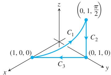
-
Zero circulation Let C be the ellipse in which the plane
2 𝑥 + 3 𝑦 − 𝑧 = 0 𝑥 2 + 𝑦 2 = 1 2 𝐹 = 𝑥 𝑖 + 𝑦 𝑗 + 𝑧 𝑘 -
Flow along a curve The field
𝐹 = 𝑥 𝑦 𝑖 + 𝑦 𝑗 − 𝑦 𝑧 𝑘 ( 0 , 0 , 0 ) ( 1 , 1 , 1 ) 𝑦 = 𝑥 2
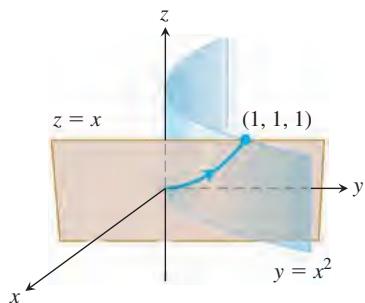
- Flow of a gradient field Find the flow of the field
𝐅 = ∇ ( 𝑥 𝑦 2 𝑧 3 )
a. Once around the curve C in Exercise 58, clockwise as viewed from above;
b. Along the line segment from
COMPUTER EXPLORATIONS
In Exercises 63–68, use a CAS to perform the following steps for finding the work done by force F over the given path:
a. Find
b. Evaluate the force F along the path.
c. Evaluate
-
𝐅 = 𝑥 𝑦 6 𝐢 + 3 𝑥 ( 𝑥 𝑦 5 + 2 ) 𝐣 ; 𝐫 ( 𝑡 ) = ( 2 c o s 𝑡 ) 𝐢 + ( s i n 𝑡 ) 𝐣 , 0 ≤ 𝑡 ≤ 2 𝜋 -
𝐅 = 3 1 + 𝑥 2 𝐢 + 2 1 + 𝑦 2 𝐣 ; 𝐫 ( 𝑡 ) = ( c o s 𝑡 ) 𝐢 + ( s i n 𝑡 ) 𝐣 ,
-
𝐅 = ( 𝑦 + 𝑦 𝑧 c o s 𝑥 𝑦 𝑧 ) 𝐢 + ( 𝑥 2 + 𝑥 𝑧 c o s 𝑥 𝑦 𝑧 ) 𝐣 + ( 𝑧 + 𝑥 𝑦 c o s 𝑥 𝑦 𝑧 ) 𝐤 ; 𝐫 ( 𝑡 ) = ( 2 c o s 𝑡 ) 𝐢 + ( 3 s i n 𝑡 ) 𝐣 + 𝐤 , 0 ≤ 𝑡 ≤ 2 𝜋 -
𝐅 = 2 𝑥 𝑦 𝐢 − 𝑦 2 𝐣 + 𝑧 𝑒 𝑥 𝐤 ; 𝐫 ( 𝑡 ) = − 𝑡 𝐢 + √ 𝑡 𝐣 + 3 𝑡 𝐤 , 1 ≤ 𝑡 ≤ 4 -
𝐅 = ( 2 𝑦 + s i n 𝑥 ) 𝐢 + ( 𝑧 2 + ( 1 / 3 ) c o s 𝑦 ) 𝐣 + 𝑥 4 𝐤 ; 𝐫 ( 𝑡 ) = ( s i n 𝑡 ) 𝐢 + ( c o s 𝑡 ) 𝐣 + ( s i n 2 𝑡 ) 𝐤 , − 𝜋 / 2 ≤ 𝑡 ≤ 𝜋 / 2 -
𝐅 = ( 𝑥 2 𝑦 ) 𝐢 + 1 3 𝑥 3 𝐣 + 𝑥 𝑦 𝐤 ; 𝐫 ( 𝑡 ) = ( c o s 𝑡 ) 𝐢 + ( s i n 𝑡 ) 𝐣 + ( 2 s i n 2 𝑡 − 1 ) 𝐤 , 0 ≤ 𝑡 ≤ 2 𝜋
15.3 Path Independence, Conservative Fields, and Potential Functions
A gravitational field G is a vector field that represents the effect of gravity at a point in space due to the presence of a massive object. The gravitational force on a body of mass m placed in the field is given by F = mG. Similarly, an electric field E is a vector field in space that represents the effect of electric forces on a charged particle placed within it. The force on a body of charge q placed in the field is given by F = qE. In gravitational and electric fields, the amount of work it takes to move a mass or charge from one point to another depends on the initial and final positions of the object—not on which path is taken between these positions. In this section we study vector fields with this independence-of-path property and the calculation of work integrals associated with them.
Path Independence
If
DEFINITIONS Let F be a vector field defined on an open region D in space, and suppose that for any two points A and B in D, the line integral
along a path C from A to B in D is the same over all paths from A to B. Then the integral ∫ 𝐶 𝐹 ⋅ 𝑑 𝑟 is path independent in D and the field F is conservative on D. ∫ 𝐶 𝐹 ⋅ 𝑑 𝑟
The word conservative comes from physics, where it refers to fields in which the principle of conservation of energy holds. When a line integral is independent of the path C from point A to point B, we sometimes represent the integral by the symbol
(a)
(b)
Not simply connected
(c)
(d)
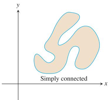
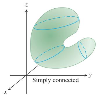
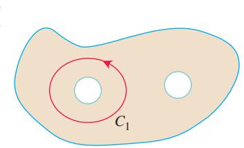
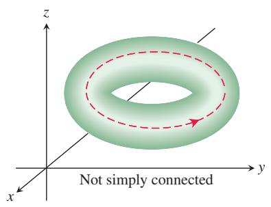
FIGURE 15.25 Four connected regions. In (a) and (b), the regions are simply connected. In (c) and (d), the regions are not simply connected because the curves
Under reasonable differentiability conditions that we will specify, we will show that a field F is conservative if and only if it is the gradient field of a scalar function f—that is, if and only if
DEFINITION If F is a vector field defined on D and
for some scalar function f on D, then f is called a potential function for F. 𝐹 = ∇ 𝑓
A gravitational potential is a scalar function whose gradient field is a gravitational field, an electric potential is a scalar function whose gradient field is an electric field, and so on. As we will see, once we have found a potential function f for a field F, we can evaluate all the line integrals in the domain of F over any path between A and B by
If you think of
Conservative fields have other important properties. For example, saying that F is conservative on D is equivalent to saying that the integral of F around every closed path in D is zero. Certain conditions on the curves, fields, and domains must be satisfied for Equation (1) to be valid. We discuss these conditions next.
Assumptions on Curves, Vector Fields, and Domains
In order for the computations and results we derive below to be valid, we must assume certain properties for the curves, surfaces, domains, and vector fields we consider. We give these assumptions in the statements of theorems, and they also apply to the examples and exercises unless otherwise stated.
The curves we consider are piecewise smooth. Such curves are made up of finitely many smooth pieces connected end to end, as discussed in Section 12.1. For such curves we can compute lengths and, except at finitely many points where the smooth pieces connect, tangent vectors. We consider vector fields F whose components have continuous first partial derivatives.
The domains D we consider are connected. For an open region, this means that any two points in D can be joined by a smooth curve that lies in the region. Some results require D to be simply connected, which means that every loop in D can be contracted to a point in D without ever leaving D. The plane with a disk removed is a two-dimensional region that is not simply connected; a loop in the plane that goes around the disk cannot be contracted to a point without going into the “hole” left by the removed disk (see Figure 15.25c). Similarly, if we remove a line from space, the remaining region D is not simply connected. A curve encircling the line cannot be shrunk to a point while remaining inside D.
Connectivity and simple connectivity are not the same, and neither property implies the other. Think of connected regions as being in “one piece” and of simply connected regions as not having any “loop-catching holes.” All of space itself is both connected and simply connected. Figure 15.25 illustrates some of these properties.
Caution Some of the results in this chapter can fail to hold if applied to situations where the conditions we’ve imposed are not met. In particular, the component test for conservative fields, given later in this section, is not valid on domains that are not simply connected (see Example 5). The condition will be stated when needed.
Line Integrals in Conservative Fields
A gradient field F is obtained by differentiating a scalar function f. A theorem analogous to the Fundamental Theorem of Calculus gives a way to evaluate the line integrals of gradient fields.
Like the Fundamental Theorem of Calculus, Theorem 1 gives a direct way to evaluate line integrals without having to take limits of Riemann sums and without needing to compute a line integral by the procedure used in Section 15.2. Before proving Theorem 1, we give an example.
THEOREM 1—Fundamental Theorem of Line Integrals
Let C be a smooth curve joining the point A to the point B in the plane or in space and parametrized by
EXAMPLE 1 Suppose the force field
Find the work done by
Solution An application of Theorem 1 shows that the work done by F along any smooth curve C joining the two points and not passing through the origin is
The gravitational force due to a planet, and the electric force associated with a charged particle, can both be modeled by the field F given in Example 1 up to a constant that depends on the units of measurement. When used to model gravity, the function f in Example 1 represents gravitational potential energy. The sign of f is negative, and f approaches
Proof of Theorem 1 Suppose that A and B are two points in the region D and that
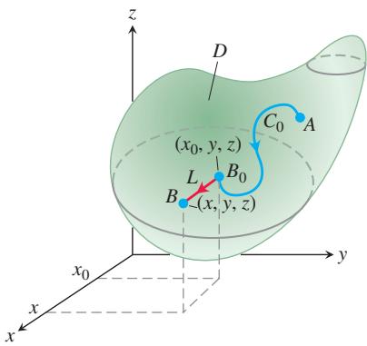
FIGURE 15.26 The function
We see from Theorem 1 that the line integral of a gradient field
THEOREM 2—Conservative Fields Are Gradient Fields
Let
Theorem 2 says that
Proof of Theorem 2 If F is a gradient field, then
On the other hand, suppose that
Suppose that B has coordinates
Differentiating, we have
Only the last term on the right depends on x, so
Now we parametrize
by the Fundamental Theorem of Calculus. The partial derivatives
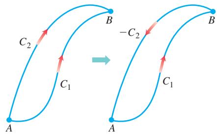
FIGURE 15.27 If we have two paths from A to B, one of them can be reversed to make a loop.
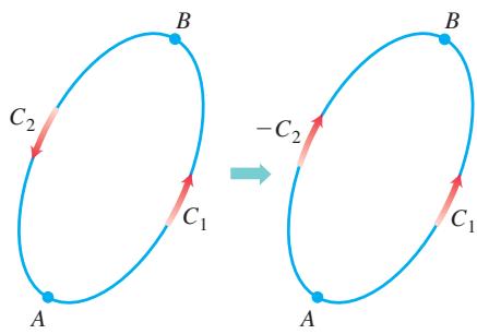
FIGURE 15.28 If A and B lie on a loop, we can reverse part of the loop to make two paths from A to B.
EXAMPLE 2 Find the work done by the conservative field
in moving an object along any smooth curve C joining the point
Solution With
A very useful property of line integrals in conservative fields comes into play when the path of integration is a closed curve, or loop. We often use the notation
THEOREM 3—Loop Property of Conservative Fields The following statements are equivalent.
∮ 𝐶 𝐹 ⋅ 𝑑 𝑟 = 0 - The field F is conservative on D.
Proof that Part 1
Thus, the integrals over
Proof that Part 2
The following diagram summarizes the results of Theorems 2 and 3.
Two questions arise:
-
How do we know whether a given vector field F is conservative?
-
If
𝐅 𝑓 𝐅 = ∇ 𝑓
Finding Potentials for Conservative Fields
The test for a vector field being conservative involves the equivalence of certain first partial derivatives of the field components.
Component Test for Conservative Fields
Let
We can view the component test as saying that on a simply connected region, the vector
is zero if and only if F is conservative. This interesting vector curl F is called the curl of F. We study it in Sections 15.4 and 15.7.
Proof that Equations (2) hold if
Hence,
The others in Equations (2) are proved similarly.
The second half of the proof, that Equations (2) imply that
Once we know that
for
as illustrated in the next example.
EXAMPLE 3 Show that
Solution The natural domain of
and calculate
The partial derivatives are continuous, so these equalities tell us that
We find
We integrate the first equation with respect to x, holding y and z fixed, to get
We write the constant of integration as a function of y and z because its value may depend on y and z, though not on x. We then calculate
so
We now calculate
SO
Hence,
We found infinitely many potential functions of
EXAMPLE 4 Show that
Solution We apply the Component Test in Equations (2) and find immediately that
The two are unequal, so F is not conservative. No further testing is required.
EXAMPLE 5 Show that the vector field
satisfies the equations in the Component Test but is not conservative over its natural domain. Explain why this is possible.
Solution We have
So it may appear that the field
To show that
Next we find
Since the line integral of
Example 5 shows that the Component Test does not apply when the domain of the field is not simply connected. However, if we change the domain in the example so that it is restricted to the ball of radius 1 centered at the point
Exact Differential Forms
It is often convenient to express work and circulation integrals in the differential form
discussed in Section 15.2. Such line integrals are relatively easy to evaluate if
Theorem 1
Thus,
just as with differentiable functions of a single variable.
DEFINITIONS Any expression
is a differential form. A differential form is exact on a domain D in space if 𝑀 ( 𝑥 , 𝑦 , 𝑧 ) 𝑑 𝑥 + 𝑁 ( 𝑥 , 𝑦 , 𝑧 ) 𝑑 𝑦 + 𝑃 ( 𝑥 , 𝑦 , 𝑧 ) 𝑑 𝑧 𝑀 𝑑 𝑥 + 𝑁 𝑑 𝑦 + 𝑃 𝑑 𝑧 = 𝜕 𝑓 𝜕 𝑥 𝑑 𝑥 + 𝜕 𝑓 𝜕 𝑦 𝑑 𝑦 + 𝜕 𝑓 𝜕 𝑧 𝑑 𝑧 = 𝑑 𝑓
for some scalar function f throughout D.
Notice that if
Component Test for Exactness of M dx + N dy + P dz
The differential form
This is equivalent to saying that the field
EXAMPLE 6 Show that
over any path from
Solution Note that the domain of
These equalities tell us that
for some function
We find
From the first equation we get
The second equation tells us that
Hence, g is a function of z alone, and
The third of Equations (5) tells us that
Therefore,
The value of the line integral is independent of the path taken from
Exercises 15.3
Testing for Conservative Fields
Which fields in Exercises 1–6 are conservative, and which are not?
Finding Potential Functions
In Exercises 7–12, find a potential function f for the field F.
Exact Differential Forms
In Exercises 13–17, show that the differential forms in the integrals are exact. Then evaluate the integrals.
-
∫ ( 2 , 3 , − 6 ) ( 0 , 0 , 0 ) 2 𝑥 𝑑 𝑥 + 2 𝑦 𝑑 𝑦 + 2 𝑧 𝑑 𝑧 -
∫ ( 3 , 5 , 0 ) ( 1 , 1 , 2 ) 𝑦 𝑧 𝑑 𝑥 + 𝑥 𝑧 𝑑 𝑦 + 𝑥 𝑦 𝑑 𝑧 -
∫ ( 1 , 2 , 3 ) ( 0 , 0 , 0 ) 2 𝑥 𝑦 𝑑 𝑥 + ( 𝑥 2 − 𝑧 2 ) 𝑑 𝑦 − 2 𝑦 𝑧 𝑑 𝑧 -
∫ ( 3 , 3 , 1 ) ( 0 , 0 , 0 ) 2 𝑥 𝑑 𝑥 − 𝑦 2 𝑑 𝑦 − 4 1 + 𝑧 2 𝑑 𝑧 -
∫ ( 0 , 1 , 1 ) ( 1 , 0 , 0 ) s i n 𝑦 c o s 𝑥 𝑑 𝑥 + c o s 𝑦 s i n 𝑥 𝑑 𝑦 + 𝑑 𝑧
Finding Potential Functions to Evaluate Line Integrals
Although they are not defined on all of space
-
∫ ( 1 , 𝜋 / 2 , 2 ) ( 0 , 2 , 1 ) 2 c o s 𝑦 𝑑 𝑥 + ( 1 𝑦 − 2 𝑥 s i n 𝑦 ) 𝑑 𝑦 + 1 𝑧 𝑑 𝑧 -
∫ ( 1 , 2 , 3 ) ( 1 , 1 , 1 ) 3 𝑥 2 𝑑 𝑥 + 𝑧 2 𝑦 𝑑 𝑦 + 2 𝑧 l n 𝑦 𝑑 𝑧 -
∫ ( 2 , 1 , 1 ) ( 1 , 2 , 1 ) ( 2 𝑥 l n 𝑦 − 𝑦 𝑧 ) 𝑑 𝑥 + ( 𝑥 2 𝑦 − 𝑥 𝑧 ) 𝑑 𝑦 − 𝑥 𝑦 𝑑 𝑧 -
∫ ( 2 , 2 , 2 ) ( 1 , 1 , 1 ) 1 𝑦 𝑑 𝑥 + ( 1 𝑧 − 𝑥 𝑦 2 ) 𝑑 𝑦 − 𝑦 𝑧 2 𝑑 𝑧 -
∫ ( 2 , 2 , 2 ) ( − 1 , − 1 , − 1 ) 2 𝑥 𝑑 𝑥 + 2 𝑦 𝑑 𝑦 + 2 𝑧 𝑑 𝑧 𝑥 2 + 𝑦 2 + 𝑧 2
Applications and Examples
- Revisiting Example 6 Evaluate the integral
from Example 6 by finding parametric equations for the line segment from
- Evaluate
along the line segment C joining
Independence of path Show that the values of the integrals in Exercises 25 and 26 do not depend on the path taken from A to B.
-
∫ 𝐵 𝐴 𝑧 2 𝑑 𝑥 + 2 𝑦 𝑑 𝑦 + 2 𝑥 𝑧 𝑑 𝑧 -
∫ 𝐵 𝐴 𝑥 𝑑 𝑥 + 𝑦 𝑑 𝑦 + 𝑧 𝑑 𝑧 √ 𝑥 2 + 𝑦 2 + 𝑧 2
In Exercises 27 and 28, find a potential function for
-
𝐅 = 2 𝑥 𝑦 𝐢 + ( 1 − 𝑥 2 𝑦 2 ) 𝐣 , { ( 𝑥 , 𝑦 ) : 𝑦 > 0 } -
𝐅 = ( 𝑒 𝑥 l n 𝑦 ) 𝐢 + ( 𝑒 𝑥 𝑦 + s i n 𝑧 ) 𝐣 + ( 𝑦 c o s 𝑧 ) 𝐤 -
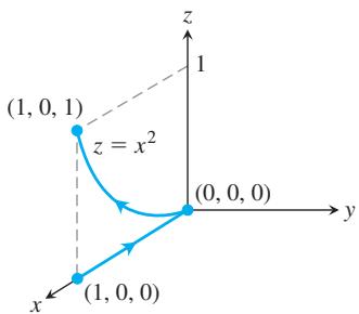
Work along different paths Find the work done by
𝐅 = ( 𝑥 2 + 𝑦 ) 𝐢 + ( 𝑦 2 + 𝑥 ) 𝐣 + 𝑧 𝑒 𝑧 𝐤 ( 1 , 0 , 0 ) ( 1 , 0 , 1 )
a. The line segment
- Work along different paths Find the work done by
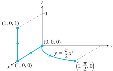
𝐅 = 𝑒 𝑦 𝑧 𝐢 + ( 𝑥 𝑧 𝑒 𝑦 𝑧 + 𝑧 c o s 𝑦 ) 𝐣 + ( 𝑥 𝑦 𝑒 𝑦 𝑧 + s i n 𝑦 ) 𝐤 ( 1 , 0 , 1 ) ( 1 , 𝜋 / 2 , 0 )
a. The line segment
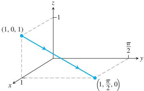
b. The line segment from
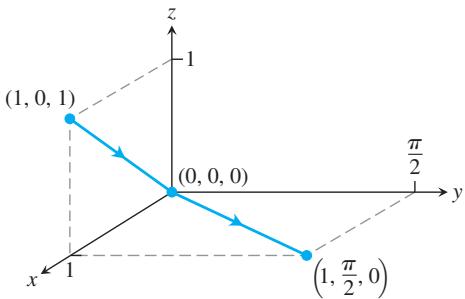
c. The line segment from
- Evaluating a work integral two ways Let
𝐅 = ∇ ( 𝑥 3 𝑦 2 ) 𝐶 𝑥 𝑦 ( − 1 , 1 ) ( 1 , 1 ) ( − 1 , 1 ) ( 0 , 0 ) ( 0 , 0 ) ( 1 , 1 ) ∫ 𝐶 𝐅 ⋅ 𝑑 𝑟
a. Find parametrizations for the segments that make up C and evaluate the integral.
b. Use
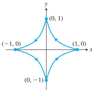
- Integral along different paths Evaluate the line integral
∫ 𝐶 2 𝑥 c o s 𝑦 𝑑 𝑥 − 𝑥 2 s i n 𝑦 𝑑 𝑦 𝐶
a. The parabola
b. The line segment from
c. The x-axis from
d. The astroid
- a. Exact differential form How are the constants
𝑎 , 𝑏 𝑐
b. Gradient field For what values of
be a gradient field?
- Gradient of a line integral Suppose that
𝐅 = ∇ 𝑓
Show that
-
Path of least work You have been asked to find the path along which a force field F will perform the least work in moving a particle between two locations. A quick calculation on your part shows F to be conservative. How should you respond? Give reasons for your answer.
-
A revealing experiment By experiment, you find that a force field
𝐅 𝐶 1 𝐴 𝐵 𝐶 2 𝐴 𝐵 𝐅 -
Work by a constant force Show that the work done by a constant force field
𝐅 = 𝑎 𝑖 + 𝑏 𝑗 + 𝑐 𝑘 𝐴 𝐵 𝑊 = 𝐅 ⋅ ⟶ 𝐴 𝐵 -
Gravitational field
a. Find a potential function for the gravitational field
15.4 Green’s Theorem in the Plane
b. Let
If
The discussion is given in terms of velocity fields of fluid flows (a fluid is a liquid or a gas) because they are easy to visualize. However, Green’s Theorem applies to any vector field, independent of any particular interpretation of the field, provided the assumptions of the theorem are satisfied. We introduce two new ideas for Green’s Theorem: circulation density around an axis perpendicular to the plane and divergence (or flux density).
Spin Around an Axis: The k-Component of Curl
Suppose that
that, along with its interior, lies entirely in
and the rectangle A in Figure 15.29 (where we assume both components of F are positive).
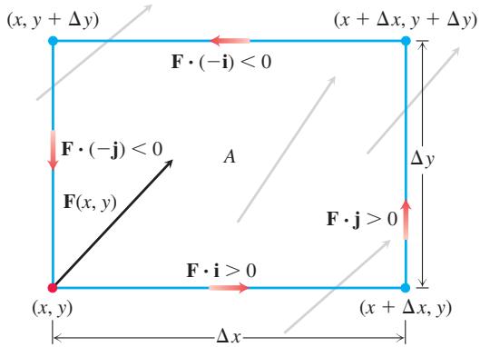
FIGURE 15.29 The rate at which a fluid flows along the bottom edge of a rectangular region A in the direction i is approximately
The circulation rate of F around the boundary of A is the sum of flow rates along the sides in the tangential direction. For the bottom edge, the flow rate is approximately
This is the scalar component of the velocity
Bottom:
Right:
Left:
We sum opposite pairs to get
Top and bottom:
Right and left:
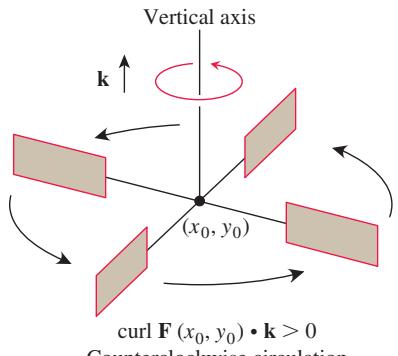
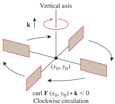
FIGURE 15.30 In the flow of an incompressible fluid over a plane region, the k-component of the curl measures the rate of the fluid’s rotation at a point. The k-component of the curl is positive at points where the rotation is counterclockwise and negative where the rotation is clockwise.
Adding these last two equations gives the net circulation rate relative to the counterclockwise orientation,
We now divide by
We let
If we see a counterclockwise rotation looking downward onto the xy-plane from the tip of the unit k vector, then the circulation density is positive (Figure 15.30).
DEFINITION The circulation density of a vector field
at the point 𝐅 = 𝑀 𝐢 + 𝑁 𝐣 is the scalar expression ( 𝑥 , 𝑦 ) 𝜕 𝑁 𝜕 𝑥 − 𝜕 𝑀 𝜕 𝑦 . ( 1 )
The expression in Equation (1) is the the k-component of the curl of F, which was introduced in Equation (3) of Section 15.3:
If water is moving about a region in the xy-plane in a thin layer, then the k-component of the curl at a point
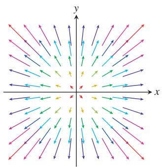
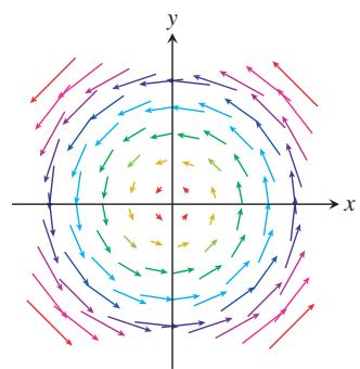
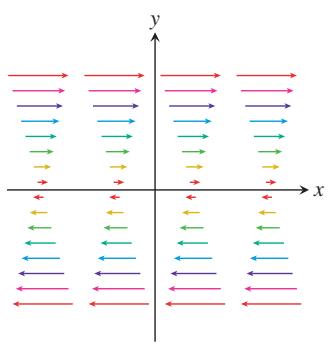
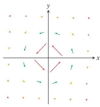
EXAMPLE 1 The following vector fields represent the velocity of a gas flowing in the xy-plane. Find the circulation density of each vector field and interpret its physical meaning. Figure 15.31 displays the vector fields.
(a) Uniform expansion or compression:
(b) Uniform rotation:
(c) Shearing flow:
(d) Whirlpool effect:
Solution
(a) Uniform expansion: (curl
(b) Rotation: (curl
(a)
(b)
(c)
(d)
FIGURE 15.31 Velocity fields of a gas flowing in the plane (Example 1).
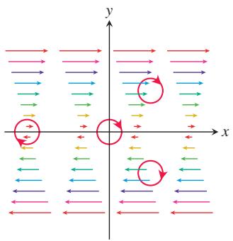
(c) Shear: (curl
FIGURE 15.32 A shearing flow pushes the fluid clockwise around each point (Example 1c).
(d) Whirlpool:
The circulation density is 0 at every point away from the origin (where the vector field is undefined and the whirlpool effect blows up), and the gas is not circulating at any point for which the vector field is defined.
One form of Green’s Theorem tells us how circulation density can be used to calculate the line integral for flow in the
Divergence
Consider again the velocity field
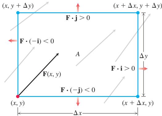
FIGURE 15.33 The rate at which the fluid leaves the rectangular region A across the bottom edge in the direction of the outward normal -j is approximately
The rate at which fluid leaves the rectangle across the bottom edge is approximately (Figure 15.33)
This is the scalar component of the velocity at
Fluid Flow Rates:
Bottom:
Summing opposite pairs gives
Top and bottom:
Right and left:
Adding these last two equations gives the net effect of the flow rates, or the
Flux across rectangle boundary
We now divide by
div
Sink: div
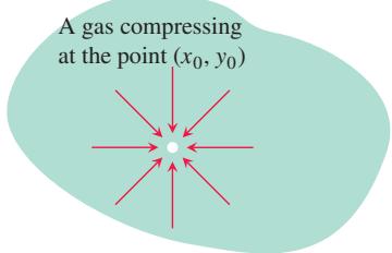
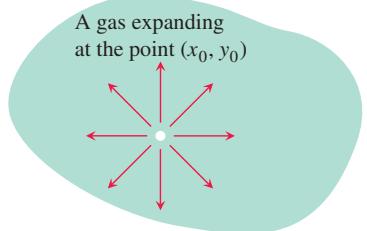
FIGURE 15.34 If a gas is expanding at a point
Finally, we let
DEFINITION The divergence (flux density) of a vector field
at the point 𝐅 = 𝑀 𝐢 + 𝑁 𝐣 is ( 𝑥 , 𝑦 ) d i v 𝐅 = 𝜕 𝑀 𝜕 𝑥 + 𝜕 𝑁 𝜕 𝑦 . ( 2 )
A gas is compressible, unlike a liquid, and the divergence of its velocity field measures to what extent it is expanding or compressing at each point. Intuitively, if a gas is expanding at the point
EXAMPLE 2 Find the divergence, and interpret what it means, for each vector field in Example 1 representing the velocity of a gas flowing in the xy-plane.
Solution
(a)
(b) div
(c) div
(d) div
Cases (b), (c), and (d) of Figure 15.31 are plausible models for the two-dimensional flow of a liquid. In fluid dynamics, when the velocity field of a flowing fluid always has divergence equal to zero, as in those cases, the flow is said to be incompressible.
Two Forms for Green’s Theorem
A simple closed curve C can be traversed in two possible directions. (Recall that a curve is simple if it does not cross itself.) The curve is traversed counterclockwise, and said to be positively oriented, if the region it encloses is always to the left when moving along the curve. If the curve is traversed clockwise, then the enclosed region is on the right when moving along the curve, and the curve is said to be negatively oriented. The line integral of a vector field F along C reverses sign if we change the orientation. We use the notation
for the line integral when the simple closed curve C is traversed counterclockwise, with its positive orientation.
In one form, Green’s Theorem says that the counterclockwise circulation of a vector field around a simple closed curve is the double integral of the k-component of the curl of the field over the region enclosed by the curve. Recall the defining Equation (5) for circulation in Section 15.2.
Circulation around
(curl
Flux of
THEOREM 4—Green’s Theorem (Circulation-Curl or Tangential Form)
Let C be a piecewise smooth, simple closed curve enclosing a region R in the plane. Let
A second form of Green’s Theorem says that the outward flux of a vector field across a simple closed curve in the plane equals the double integral of the divergence of the field over the region enclosed by the curve. Recall the formulas for flux in Equations (8) and (9) in Section 15.2.
THEOREM 5—Green’s Theorem (Flux-Divergence or Normal Form)
Let C be a piecewise smooth, simple closed curve enclosing a region R in the plane. Let
The two forms of Green’s Theorem are equivalent. Applying Equation (3) to the field
Both forms of Green’s Theorem can be viewed as two-dimensional generalizations of the Fundamental Theorem of Calculus from Section 5.4. The counterclockwise circulation of
EXAMPLE 3 Verify both forms of Green’s Theorem for the vector field
and the region R bounded by the unit circle
Solution First we evaluate the counterclockwise circulation of
Therefore,
This gives the left side of Equation (3). Next we find the curl integral, the right side of Equation (3). Since M = x - y and N = x, we have
Therefore,
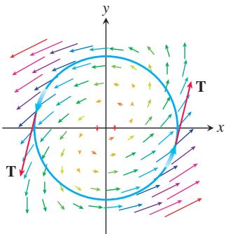
Thus, the right and left sides of Equation (3) both equal
FIGURE 15.35 The vector field in Example 3 has a counterclockwise circulation of
Figure 15.35 displays the vector field and circulation around C.
Now we compute the two sides of Equation (4) in the flux-divergence form of Green’s Theorem, starting with the outward flux:
Next we compute the divergence integral:
Hence the right and left sides of Equation (4) both equal
Using Green’s Theorem to Evaluate Line Integrals
If we construct a closed curve
EXAMPLE 4 Evaluate the line integral
where C is the boundary of the square
Solution We can use either form of Green’s Theorem to change the line integral into a double integral over the square, where
- With the Tangential Form Equation (3): Taking
𝑀 = − 𝑦 2 𝑁 = 𝑥 𝑦
- With the Normal Form Equation (4): Taking M = xy,
𝑁 = 𝑦 2
EXAMPLE 5 Calculate the outward flux of the vector field
Solution Calculating the flux with a line integral would take four integrations, one for each side of the square. With Green’s Theorem, we can change the line integral to one double integral. With
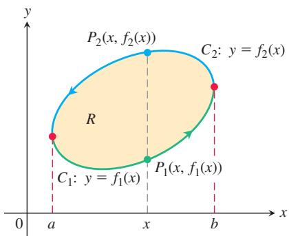
FIGURE 15.36 The boundary curve C is made up of
Proof of Green’s Theorem for Special Regions
Let
Figure 15.36 shows C made up of two directed parts:
For any
(c)
We can then integrate this with respect to x from a to b:
Therefore, reversing the order of the equations, we have
(6)
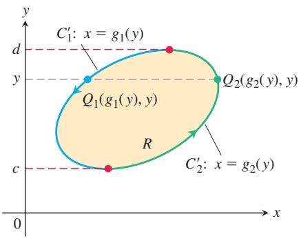
Equation (6) is half the result we need for Equation (5). We derive the other half by integrating
Summing Equations (6) and (7) gives Equation (5). This concludes the proof.
FIGURE 15.37 The boundary curve
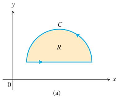
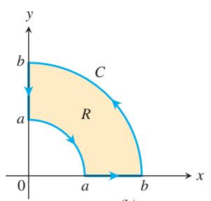
Green’s Theorem also holds for more general regions, such as those shown in Figure 15.38. Notice that the region in Figure 15.38c is not simply connected. The curves
(b)
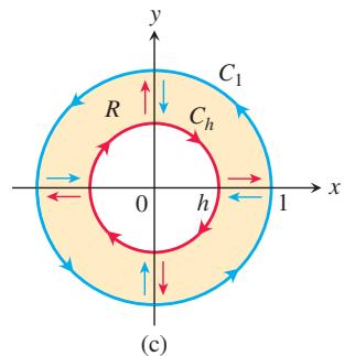
FIGURE 15.38 Other regions to which Green’s Theorem applies. In (c) the axes convert the region into four simply connected regions, and we sum the line integrals along the oriented boundaries.
Exercises 15.4
Computing the k-Component of Curl(F)
In Exercises 1–6, find the k-component of
-
𝐅 = ( 𝑥 + 𝑦 ) 𝐢 + ( 2 𝑥 𝑦 ) 𝐣 -
𝐅 = ( 𝑥 2 − 𝑦 ) 𝐢 + ( 𝑦 2 ) 𝐣 -
𝐅 = ( 𝑥 𝑒 𝑦 ) 𝐢 + ( 𝑦 𝑒 𝑥 ) 𝐣 -
𝐅 = ( 𝑥 2 𝑦 ) 𝐢 + ( 𝑥 𝑦 2 ) 𝐣 -
𝐅 = ( 𝑦 s i n 𝑥 ) 𝐢 + ( 𝑥 s i n 𝑦 ) 𝐣 -
𝐅 = ( 𝑥 / 𝑦 ) 𝐢 − ( 𝑦 / 𝑥 ) 𝐣
Verifying Green’s Theorem
In Exercises 7–10, verify the conclusion of Green’s Theorem by evaluating both sides of Equations (3) and (4) for the field
Circulation and Flux
In Exercises 11–20, use Green’s Theorem to find the counterclockwise circulation and outward flux for the field F and the curve C.
𝐅 = ( 𝑥 − 𝑦 ) 𝐢 + ( 𝑦 − 𝑥 ) 𝐣
C: The square bounded by x = 0, x = 1, y = 0, and y = 1
𝐅 = ( 𝑥 2 + 4 𝑦 ) 𝐢 + ( 𝑥 + 𝑦 2 ) 𝐣
C: The square bounded by x = 0, x = 1, y = 0, and y = 1
𝐅 = ( 𝑦 2 − 𝑥 2 ) 𝐢 + ( 𝑥 2 + 𝑦 2 ) 𝐣
C: The triangle bounded by y = 0, x = 3, and y = x
𝐅 = ( 𝑥 + 𝑦 ) 𝐢 − ( 𝑥 2 + 𝑦 2 ) 𝐣
C: The triangle bounded by y = 0, x = 1, and y = x
-
𝐅 = ( 𝑥 𝑦 + 𝑦 2 ) 𝐢 + ( 𝑥 − 𝑦 ) 𝐣 -
𝐅 = ( 𝑥 + 3 𝑦 ) 𝐢 + ( 2 𝑥 − 𝑦 ) 𝐣
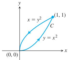
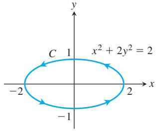
𝐅 = 𝑥 3 𝑦 2 𝐢 + 1 2 𝑥 4 𝑦 𝐣
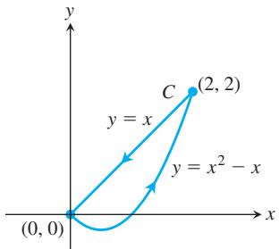
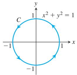
𝐅 = ( 𝑥 + 𝑒 𝑥 s i n 𝑦 ) 𝐢 + ( 𝑥 + 𝑒 𝑥 c o s 𝑦 ) 𝐣
C: The right-hand loop of the lemniscate
𝐅 = ( t a n − 1 𝑦 𝑥 ) 𝐢 + l n ( 𝑥 2 + 𝑦 2 ) 𝐣
C: The boundary of the region defined by the polar coordinate inequalities
-
Find the counterclockwise circulation and outward flux of the field
𝐹 = 𝑥 𝑦 𝐢 + 𝑦 2 𝐣 𝑦 = 𝑥 2 -
Find the counterclockwise circulation and the outward flux of the field
𝐅 = ( − s i n 𝑦 ) 𝐢 + ( 𝑥 c o s 𝑦 ) 𝐣 0 ≤ 𝑥 ≤ 𝜋 / 2 0 ≤ 𝑦 ≤ 𝜋 / 2 -
Find the outward flux of the field
across the cardioid
- Find the counterclockwise circulation of
𝐅 = ( 𝑦 + 𝑒 𝑥 l n 𝑦 ) 𝐢 + ( 𝑒 𝑥 / 𝑦 ) 𝐣 𝑦 = 3 − 𝑥 2 𝑦 = 𝑥 4 + 1
Work
In Exercises 25 and 26, find the work done by F in moving a particle once counterclockwise around the given curve.
𝐅 = 2 𝑥 𝑦 3 𝐢 + 4 𝑥 2 𝑦 2 𝐣
C: The boundary of the “triangular” region in the first quadrant enclosed by the x-axis, the line x = 1, and the curve
𝐅 = ( 4 𝑥 − 2 𝑦 ) 𝐢 + ( 2 𝑥 − 4 𝑦 ) 𝐣
C: The circle
Using Green’s Theorem
Apply Green’s Theorem to evaluate the integrals in Exercises 27–30.
∮ 𝐶 ( 𝑦 2 𝑑 𝑥 + 𝑥 2 𝑑 𝑦 )
C: The boundary of the triangle enclosed by the lines
∮ 𝐶 ( 3 𝑦 𝑑 𝑥 + 2 𝑥 𝑑 𝑦 )
C: The boundary of
∮ 𝐶 ( 6 𝑦 + 𝑥 ) 𝑑 𝑥 + ( 𝑦 + 2 𝑥 ) 𝑑 𝑦
C: The circle
∮ 𝐶 ( 2 𝑥 + 𝑦 2 ) 𝑑 𝑥 + ( 2 𝑥 𝑦 + 3 𝑦 ) 𝑑 𝑦
C: Any simple closed curve in the plane for which Green’s Theorem holds
Calculating Area with Green’s Theorem If a simple closed curve
Green’s Theorem Area Formula
The reason is that, by Equation (4) run backward,
Use the Green’s Theorem area formula given above to find the areas of the regions enclosed by the curves in Exercises 31–34.
-
The circle
𝐫 ( 𝑡 ) = ( 𝑎 c o s 𝑡 ) 𝐢 + ( 𝑎 s i n 𝑡 ) 𝐣 , 0 ≤ 𝑡 ≤ 2 𝜋 -
The ellipse
𝐫 ( 𝑡 ) = ( 𝑎 c o s 𝑡 ) 𝐢 + ( 𝑏 s i n 𝑡 ) 𝐣 , 0 ≤ 𝑡 ≤ 2 𝜋 -
The astroid
𝐫 ( 𝑡 ) = ( c o s 3 𝑡 ) 𝐢 + ( s i n 3 𝑡 ) 𝐣 , 0 ≤ 𝑡 ≤ 2 𝜋 -
One arch of the cycloid
𝑥 = 𝑡 − s i n 𝑡 𝑦 = 1 − c o s 𝑡 -
Let
𝐶
a.
b.
- Integral dependent only on area Show that the value of
around any square depends only on the area of the square and not on its location in the plane.
- Evaluate the integral
for any closed path
- Evaluate the integral
for any closed path
- Area as a line integral Show that if
𝑅 𝐶
then
for all closed curves
- Maximizing work Among all smooth, simple closed curves in the plane, oriented counterclockwise, find the one along which the work done by
is greatest. (Hint: Where is (curl F) · k positive?)
- Regions with many holes Green’s Theorem holds for a region
𝑅 𝑅
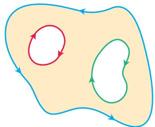
a. Let
b. Let
has two possible values, depending on whether
-
Bendixson’s criterion The streamlines of a planar fluid flow are the smooth curves traced by the fluid’s individual particles. The vectors
𝐅 = 𝑀 ( 𝑥 , 𝑦 ) 𝐢 + 𝑁 ( 𝑥 , 𝑦 ) 𝐣 𝑅 𝑀 𝑥 + 𝑁 𝑦 ≠ 0 𝑅 𝑅 𝑅 𝑀 𝑥 + 𝑁 𝑦 ≠ 0 -
Establish Equation (7) to finish the proof of the special case of Green’s Theorem.
-
Curl component of conservative fields Can anything be said about the curl component of a conservative two-dimensional vector field? Give reasons for your answer.
COMPUTER EXPLORATIONS
In Exercises 49–52, use a CAS and Green’s Theorem to find the counterclockwise circulation of the field F around the simple closed curve C. Perform the following CAS steps.
a. Plot C in the xy-plane.
b. Determine the integrand
c. Determine the (double integral) limits of integration from your plot in part (a), and evaluate the curl integral for the circulation.
-
𝐅 = ( 2 𝑥 − 𝑦 ) 𝐢 + ( 𝑥 + 3 𝑦 ) 𝐣 , 𝐶 𝑥 2 + 4 𝑦 2 = 4 -
𝐅 = ( 2 𝑥 3 − 𝑦 3 ) 𝐢 + ( 𝑥 3 + 𝑦 3 ) 𝐣 , 𝐶 : 𝑥 2 4 + 𝑦 2 9 = 1 -
𝐹 = 𝑥 − 1 𝑒 𝑦 𝑖 + ( 𝑒 𝑦 l n 𝑥 + 2 𝑥 ) 𝑗 ,
C: The boundary of the region defined by
𝐹 = 𝑥 𝑒 𝑦 𝑖 + ( 4 𝑥 2 l n 𝑦 ) 𝑗 ,
C: The triangle with vertices
15.5 Surfaces and Area
We have described curves in the plane in three different ways.
Explicit form:
Implicit form:
Parametric vector form:
We have analogous descriptions of surfaces in space.
Explicit form:
Implicit form:
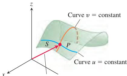
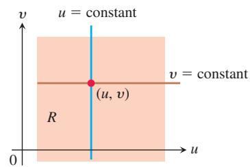
FIGURE 15.39 A parametrized surface S expressed as a vector function of two variables defined on a region R.
There is also a parametric form for surfaces that gives the position of a point on the surface as a vector function of two variables. We discuss this new form in this section and apply the form to obtain the area of a surface as a double integral. Double integral formulas for areas of surfaces given in implicit and explicit forms are then obtained as special cases of the more general parametric formula.
Parametrizations of Surfaces
Suppose
is a continuous vector function that is defined on a region R in the uv-plane and is one-to-one on the interior of R (Figure 15.39). We call the range of r the surface S defined or traced by r. Equation (1) together with the domain R constitutes a parametrization of the surface. The variables u and v are the parameters, and R is the parameter domain. To simplify our discussion, we take R to be a rectangle defined by inequalities of the form
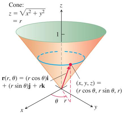
FIGURE 15.40 The cone in Example 1 can be parametrized using cylindrical coordinates.
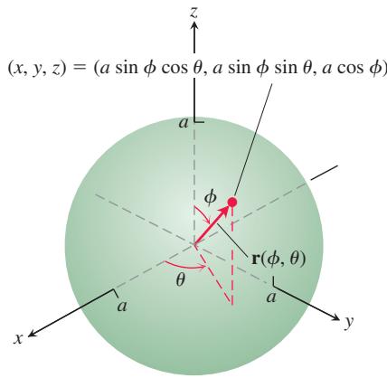
FIGURE 15.41 The sphere in Example 2 can be parametrized using spherical coordinates.
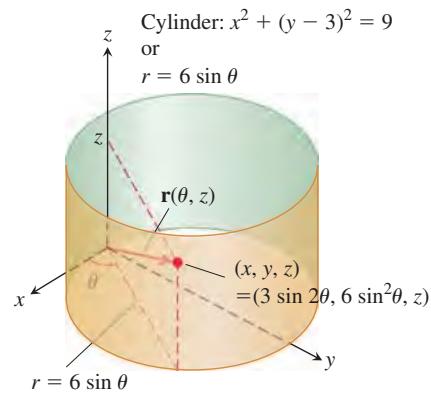
FIGURE 15.42 The cylinder in Example 3 can be parametrized using cylindrical coordinates.
EXAMPLE 1 Find a parametrization of the cone
Solution Here, cylindrical coordinates provide a parametrization. A typical point
The parametrization is one-to-one on the interior of the domain, though not on the boundary where r = 0 (mapped to the tip of the cone) or where
EXAMPLE 2 Find a parametrization of the sphere
Solution Spherical coordinates provide what we need. A typical point
Again, the parametrization is one-to-one on the interior of the domain, though not on its boundary.
EXAMPLE 3 Find a parametrization of the cylinder
Solution In cylindrical coordinates, a point
or
A typical point on the cylinder therefore has
Taking
which is one-to-one on the interior of the domain.
Surface Area
Our goal is to find a double integral that gives the area of a curved surface S based on the parametrization
We need S to be smooth for the construction we now describe. The definition of smoothness involves the partial derivatives of r with respect to u and v:
DEFINITION A parametrized surface
is smooth if 𝐫 ( 𝑢 , 𝑣 ) = 𝑓 ( 𝑢 , 𝑣 ) 𝐢 + 𝑔 ( 𝑢 , 𝑣 ) 𝐣 + ℎ ( 𝑢 , 𝑣 ) 𝐤 and 𝑟 𝑢 are continuous and if 𝑟 𝑣 is never zero on the interior of the parameter domain. 𝑟 𝑢 × 𝑟 𝑣
The condition that
Now consider a small rectangle
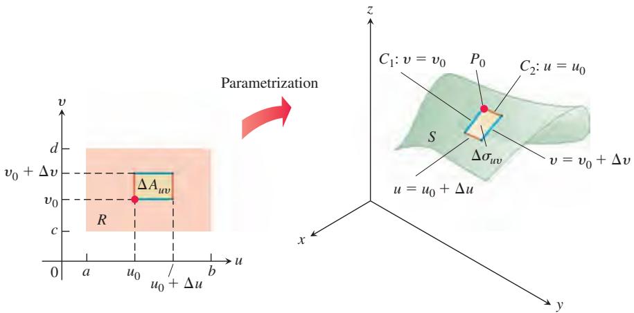
FIGURE 15.43 A rectangular area element
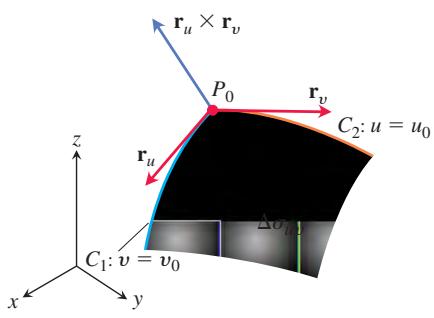
FIGURE 15.44 A magnified view of a surface patch element
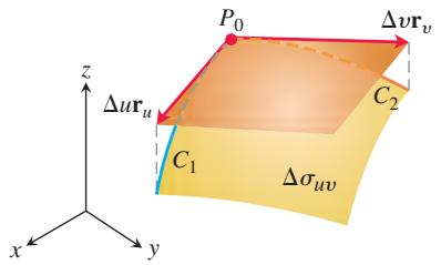
FIGURE 15.45 The area of the parallelogram determined by the vectors
Figure 15.44 shows an enlarged view of
We next approximate the surface patch element
A partition of the region R in the uv-plane by rectangular regions
As
DEFINITION The area of the smooth surface
𝐫 ( 𝑢 , 𝑣 ) = 𝑓 ( 𝑢 , 𝑣 ) 𝐢 + 𝑔 ( 𝑢 , 𝑣 ) 𝐣 + ℎ ( 𝑢 , 𝑣 ) 𝐤 , 𝑎 ≤ 𝑢 ≤ 𝑏 , 𝑐 ≤ 𝑣 ≤ 𝑑 is
𝐴 = ∬ 𝑅 | 𝐫 𝑢 × 𝐫 𝑣 | 𝑑 𝐴 = ∫ 𝑑 𝑐 ∫ 𝑏 𝑎 | 𝐫 𝑢 × 𝐫 𝑣 | 𝑑 𝑢 𝑑 𝑣 . ( 4 )
We can abbreviate the integral in Equation (4) by writing
Surface Area Differential for a Parametrized Surface
Surface area differential, also called surface area element
Differential formula for surface area
EXAMPLE 4 Find the surface area of the cone in Example 1 (Figure 15.40).
Solution In Example 1, we found the parametrization
To apply Equation (4), we first find
Thus,
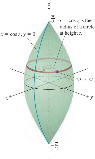
FIGURE 15.46 The “football” surface in Example 6 obtained by rotating the curve x = cos z about the z-axis.
EXAMPLE 5 Find the surface area of a sphere of radius a.
Solution We use the parametrization from Example 2:
For
Thus,
because
This gives the well-known formula for the surface area of a sphere.
EXAMPLE 6 Let S be the “football” surface formed by rotating the curve
Solution Example 2 suggests finding a parametrization of S based on its rotation around the z-axis. If we rotate a point
Next we use Equation (5) to find the surface area of S. Differentiation of the parametrization gives
and
Computing the cross product, we have
Taking the magnitude of the cross product gives
From Equation (4) the surface area is given by the integral
To evaluate the integral, we substitute
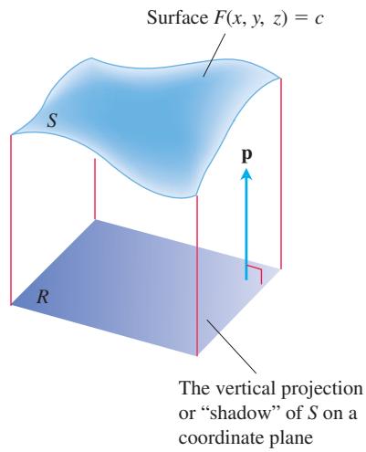
FIGURE 15.47 As we soon see, the area of a surface S in space can be calculated by evaluating a related double integral over the vertical projection or “shadow” of S on a coordinate plane. The unit vector p is normal to the plane.
Implicit Surfaces
Surfaces are often presented as level sets of a function, described by an equation such as
for some constant c. Such a level surface does not come with an explicit parametrization and is called an implicitly defined surface. Implicit surfaces arise, for example, as equipotential surfaces in electric or gravitational fields. Figure 15.47 shows a piece of such a surface. It may be difficult to find explicit formulas for the functions f, g, and h that describe the surface in the form
Figure 15.47 shows a piece of an implicit surface S that lies above its “shadow” region R in the plane beneath it. The surface is defined by the equation
Assume that the normal vector p is the unit vector k, so the region R in Figure 15.47 lies in the xy-plane. By assumption, we then have
gives a parametrization of the surface S. We use Equation (4) to find the area of S.
Calculating the partial derivatives of r, we find
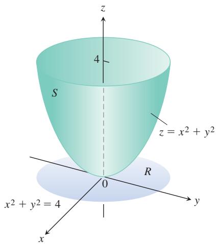
FIGURE 15.48 The area of this parabolic surface is calculated in Example 7.
Applying the Chain Rule for implicit differentiation (see Equation (2) in Section 13.4) to
Substitution of these derivatives into the derivatives of
From a routine calculation of the cross product, we find
Therefore, the surface area differential is given by
We obtain similar calculations if instead the vector
Formula for the Surface Area of an Implicit Surface
The area of the surface
where
Thus, the area is the double integral over
We reached Equation (7) under the assumption that
EXAMPLE 7 Find the area of the surface cut from the bottom of the paraboloid
Solution We sketch the surface S and the region R below it in the xy-plane (Figure 15.48). The surface S is part of the level surface
At any point
In the region R, dA = dx dy. Therefore,
Example 7 illustrates how to find the surface area for a function
EXAMPLE 8 Derive the surface area differential
Solution
(a) We parametrize the surface by taking
Computing the partial derivatives gives
Then
(b) We define the implicit function
The surface area differential derived in Example 8 gives the following formula for calculating the surface area of the graph of a function defined explicitly as
Formula for the Surface Area of a Graph
EXERCISES 15.5
Finding Parametrizations
In Exercises 1–16, find a parametrization of the surface. (There are many correct ways to do these, so your answers may not be the same as those in the back of the text.)
-
The paraboloid
𝑧 = 𝑥 2 + 𝑦 2 , 𝑧 ≤ 4 -
The paraboloid
𝑧 = 9 − 𝑥 2 − 𝑦 2 , 𝑧 ≥ 0 -
Cone frustum The first-octant portion of the cone
𝑧 = √ 𝑥 2 + 𝑦 2 / 2 𝑧 = 0 𝑧 = 3 -
Cone frustum The portion of the cone
𝑧 = 2 √ 𝑥 2 + 𝑦 2 -
Spherical cap The cap cut from the sphere
𝑥 2 + 𝑦 2 + 𝑧 2 = 9 𝑧 = √ 𝑥 2 + 𝑦 2 -
Spherical cap The portion of the sphere
𝑥 2 + 𝑦 2 + 𝑧 2 = 4 𝑧 = √ 𝑥 2 + 𝑦 2 -
Spherical band The portion of the sphere
𝑥 2 + 𝑦 2 + 𝑧 2 = 3 𝑧 = √ 3 / 2 𝑧 = − √ 3 / 2 -
Spherical cap The upper portion cut from the sphere
𝑥 2 + 𝑦 2 + 𝑧 2 = 8 𝑧 = − 2 -
Parabolic cylinder between planes The surface cut from the parabolic cylinder
𝑧 = 4 − 𝑦 2 𝑥 = 0 , 𝑥 = 2 𝑧 = 0 -
Parabolic cylinder between planes The surface cut from the parabolic cylinder
𝑦 = 𝑥 2 𝑧 = 0 , 𝑧 = 3 𝑦 = 2 -
Circular cylinder band The portion of the cylinder
𝑦 2 + 𝑧 2 = 9 -
Circular cylinder band The portion of the cylinder
𝑥 2 + 𝑧 2 = 4 -
Tilted plane inside cylinder The portion of the plane
𝑥 + 𝑦 + 𝑧 = 1
a. Inside the cylinder
b. Inside the cylinder
- Tilted plane inside cylinder The portion of the plane
𝑥 − 𝑦 + 2 𝑧 = 2
a. Inside the cylinder
b. Inside the cylinder
-
Circular cylinder band The portion of the cylinder
( 𝑥 − 2 ) 2 + 𝑧 2 = 4 -
Circular cylinder band The portion of the cylinder
𝑦 2 + ( 𝑧 − 5 ) 2 = 2 5
Surface Area of Parametrized Surfaces
In Exercises 17–26, use a parametrization to express the area of the surface as a double integral. Then evaluate the integral. (There are many correct ways to set up the integrals, so your integrals may not be the same as those in the back of the text. They should have the same values, however.)
-
Tilted plane inside cylinder The portion of the plane
𝑦 + 2 𝑧 = 2 𝑥 2 + 𝑦 2 = 1 -
Plane inside cylinder The portion of the plane
𝑧 = − 𝑥 𝑥 2 + 𝑦 2 = 4 -
Cone frustum The portion of the cone
𝑧 = 2 √ 𝑥 2 + 𝑦 2 𝑧 = 2 𝑧 = 6 -
Cone frustum The portion of the cone
𝑧 = √ 𝑥 2 + 𝑦 2 / 3 𝑧 = 1 𝑧 = 4 / 3 -
Circular cylinder band The portion of the cylinder
𝑥 2 + 𝑦 2 = 1 -
Circular cylinder band The portion of the cylinder
𝑥 2 + 𝑧 2 = 1 0 𝑦 = − 1 𝑦 = 1 -
Parabolic cap The cap cut from the paraboloid
𝑧 = 2 − 𝑥 2 − 𝑦 2 𝑧 = √ 𝑥 2 + 𝑦 2 -
Parabolic band The portion of the paraboloid
𝑧 = 𝑥 2 + 𝑦 2 𝑧 = 1 𝑧 = 4 -
Sawed-off sphere The lower portion cut from the sphere
𝑥 2 + 𝑦 2 + 𝑧 2 = 2 𝑧 = √ 𝑥 2 + 𝑦 2 -
Spherical band The portion of the sphere
𝑥 2 + 𝑦 2 + 𝑧 2 = 4 𝑧 = − 1 𝑧 = √ 3
Planes Tangent to Parametrized Surfaces
The tangent plane at a point
-
Cone The cone
𝐫 ( 𝑟 , 𝜃 ) = ( 𝑟 c o s 𝜃 ) 𝐢 + ( 𝑟 s i n 𝜃 ) 𝐣 + 𝑟 𝐤 , 𝑟 ≥ 0 , 0 ≤ 𝜃 ≤ 2 𝜋 𝑃 0 ( √ 2 , √ 2 , 2 ) ( 𝑟 , 𝜃 ) = ( 2 , 𝜋 / 4 ) -
Hemisphere The hemisphere surface
𝐫 ( 𝜙 , 𝜃 ) = ( 4 s i n 𝜙 c o s 𝜃 ) 𝐢 + ( 4 s i n 𝜙 s i n 𝜃 ) 𝐣 + ( 4 c o s 𝜙 ) 𝐤 , 0 ≤ 𝜙 ≤ 𝜋 / 2 , 0 ≤ 𝜃 ≤ 2 𝜋 , 𝑃 0 ( √ 2 , √ 2 , 2 √ 3 ) ( 𝜙 , 𝜃 ) = ( 𝜋 / 6 , 𝜋 / 4 ) -
Circular cylinder The circular cylinder
𝐫 ( 𝜃 , 𝑧 ) = ( 3 s i n 2 𝜃 ) 𝐢 + ( 6 s i n 2 𝜃 ) 𝐣 + 𝑧 𝐤 , 0 ≤ 𝜃 ≤ 𝜋 𝑃 0 ( 3 √ 3 / 2 , 9 / 2 , 0 ) ( 𝜃 , 𝑧 ) = ( 𝜋 / 3 , 0 ) -
Parabolic cylinder The parabolic cylinder surface
𝐫 ( 𝑥 , 𝑦 ) = 𝑥 𝐢 + 𝑦 𝐣 − 𝑥 2 𝐤 , − ∞ < 𝑥 < ∞ , − ∞ < 𝑦 < ∞ , 𝑃 0 ( 1 , 2 , − 1 ) ( 𝑥 , 𝑦 ) = ( 1 , 2 )
More Parametrizations of Surfaces
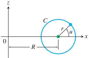
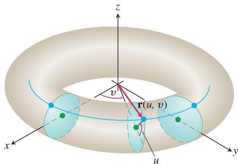
- a. A torus of revolution (doughnut) is obtained by rotating a circle C in the xz-plane about the z-axis in space. (See the accompanying figure.) If C has radius r > 0 and center
( 𝑅 , 0 , 0 )
where
b. Show that the surface area of the torus is
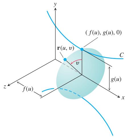
- Parametrization of a surface of revolution Suppose that the parametrized curve
𝐶 : ( 𝑓 ( 𝑢 ) , 𝑔 ( 𝑢 ) ) 𝑥 𝑔 ( 𝑢 ) > 0 𝑎 ≤ 𝑢 ≤ 𝑏
a. Show that
is a parametrization of the resulting surface of revolution, where
b. Find a parametrization for the surface obtained by revolving the curve
- a. Parametrization of an ellipsoid The parametrization
𝑥 = 𝑎 c o s 𝜃 𝑦 = 𝑏 s i n 𝜃 0 ≤ 𝜃 ≤ 2 𝜋 ( 𝑥 2 / 𝑎 2 ) + ( 𝑦 2 / 𝑏 2 ) = 1 𝜃 𝜙
is a parametrization of the ellipsoid
b. Write an integral for the surface area of the ellipsoid, but do not evaluate the integral.
- Hyperboloid of one sheet
a. Find a parametrization for the hyperboloid of one sheet
b. Generalize the result in part (a) to the hyperboloid
-
(Continuation of Exercise 34.) Find a Cartesian equation for the plane tangent to the hyperboloid
𝑥 2 + 𝑦 2 − 𝑧 2 = 2 5 ( 𝑥 0 , 𝑦 0 , 0 ) 𝑥 2 0 + 𝑦 2 0 = 2 5 -
Hyperboloid of two sheets Find a parametrization of the hyperboloid of two sheets
( 𝑧 2 / 𝑐 2 ) − ( 𝑥 2 / 𝑎 2 ) − ( 𝑦 2 / 𝑏 2 ) = 1
Surface Area for Implicit and Explicit Forms
-
Find the area of the surface cut from the paraboloid
𝑥 2 + 𝑦 2 − 𝑧 = 0 𝑧 = 2 -
Find the area of the band cut from the paraboloid
𝑥 2 + 𝑦 2 − 𝑧 = 0 -
Find the area of the region cut from the plane
𝑥 + 2 𝑦 + 2 𝑧 = 5 𝑥 = 𝑦 2 𝑥 = 2 − 𝑦 2 -
Find the area of the portion of the surface
𝑥 2 − 2 𝑧 = 0 𝑥 = √ 3 -
Find the area of the surface
𝑥 2 − 2 𝑦 − 2 𝑧 = 0 -
Find the area of the cap cut from the sphere
𝑥 2 + 𝑦 2 + 𝑧 2 = 2 𝑧 = √ 𝑥 2 + 𝑦 2 -
Find the area of the ellipse cut from the plane
𝑧 = 𝑐 𝑥 𝑐 𝑥 2 + 𝑦 2 = 1 -
Find the area of the upper portion of the cylinder
𝑥 2 + 𝑧 2 = 1 𝑥 = ± 1 / 2 𝑦 = ± 1 / 2 -
Find the area of the portion of the paraboloid
𝑥 = 4 − 𝑦 2 − 𝑧 2 1 ≤ 𝑦 2 + 𝑧 2 ≤ 4 -
Find the area of the surface cut from the paraboloid
𝑥 2 + 𝑦 + 𝑧 2 = 2 -
Find the area of the surface
𝑥 2 − 2 l n 𝑥 + √ 1 5 𝑦 − 𝑧 = 0 1 ≤ 𝑥 ≤ 2 , 0 ≤ 𝑦 ≤ 1 -
Find the area of the surface
2 𝑥 3 / 2 + 2 𝑦 3 / 2 − 3 𝑧 = 0 0 ≤ 𝑥 ≤ 1 0 ≤ 𝑦 ≤ 1
Find the area of the surfaces in Exercises 49–54.
-
The surface cut from the bottom of the paraboloid
𝑧 = 𝑥 2 + 𝑦 2 𝑧 = 3 -
The surface cut from the “nose” of the paraboloid
𝑥 = 1 − 𝑦 2 − 𝑧 2 -
The portion of the cone
𝑧 = √ 𝑥 2 + 𝑦 2 𝑥 2 + 𝑦 2 = 1 9 𝑥 2 + 4 𝑦 2 = 3 6 𝑥 2 / 𝑎 2 + 𝑦 2 / 𝑏 2 = 1 𝜋 𝑎 𝑏 -
The triangle cut from the plane
2 𝑥 + 6 𝑦 + 3 𝑧 = 6 -
The surface in the first octant cut from the cylinder
𝑦 = ( 2 / 3 ) 𝑧 3 / 2 𝑥 = 1 𝑦 = 1 6 / 3 -
The portion of the plane
𝑦 + 𝑧 = 4 𝑥 = 4 − 𝑧 2 -
Use the parametrization
and Equation (5) to derive a formula for
- Let S be the surface obtained by rotating the smooth curve
𝑦 = 𝑓 ( 𝑥 ) 𝑎 ≤ 𝑥 ≤ 𝑏 𝑓 ( 𝑥 ) ≥ 0
a. Show that the vector function
is a parametrization of S, where
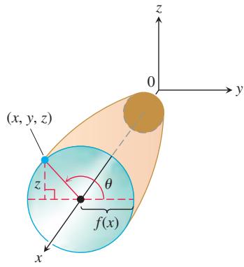
b. Use Equation (4) to show that the surface area of this surface of revolution is given by
15.6 Surface Integrals
To compute the mass of a surface, the flow of a liquid across a curved membrane, or the total electrical charge on a surface, we need to integrate a function over a curved surface in space. Such a surface integral is the two-dimensional extension of the line integral concept used to integrate over a one-dimensional curve. Like line integrals, surface integrals arise in two forms. The first occurs when we integrate a scalar function over a surface, such as integrating a mass density function defined on a surface to find its total mass. This form corresponds to line integrals of scalar functions defined in Section 15.1 and can be used to find the mass of a thin wire. The second form involves surface integrals of vector fields, analogous to the line integrals for vector fields defined in Section 15.2. An example occurs when we want to measure the net flow of a fluid across a surface submerged in the fluid (just as we previously defined the flux of F across a curve). In this section we investigate these ideas and their applications.
Surface Integrals
Suppose that the function
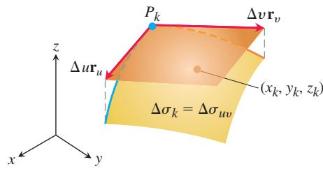
FIGURE 15.49 The area of the patch
Assume, as in Section 15.5, that the surface
In Figure 15.49, we see how a subdivision of R (considered as a rectangle for simplicity) divides the surface S into corresponding curved surface elements, or patches, of area
As we did for the subdivisions when defining double integrals in Section 14.2, we number the surface element patches in some order with their areas given by
Depending on how we pick
Notice the analogy with the definition of the double integral (Section 14.2) and with the line integral (Section 15.1). If
The formula for evaluating the surface integral depends on the manner in which S is described—parametrically, implicitly, or explicitly—as discussed in Section 15.5.
Formulas for a Surface Integral of a Scalar Function
- For a smooth surface S defined parametrically as
and a continuous function
- For a surface S given implicitly by
𝐹 ( 𝑥 , 𝑦 , 𝑧 ) = 𝑐
where p is a unit vector normal to R and
- For a surface
𝑆 𝑧 = 𝑓 ( 𝑥 , 𝑦 ) 𝑓 𝑅 𝐺 𝑆 𝑅
The surface integral in Equation (1) takes on different meanings in different applications. If G has the constant value 1, the integral gives the area of S. If G gives the mass density of a thin shell of material modeled by S, the integral gives the mass of the shell. If G gives the charge density of a thin shell, the integral gives the total charge.
EXAMPLE 1 Integrate
Solution Using Equation (2) and the calculations from Example 4 in Section 15.5, we have
Surface integrals behave like other double integrals, the integral of the sum of two functions being the sum of their integrals and so on. The domain Additivity Property takes the form
When S is partitioned by smooth curves into a finite number of smooth patches with non-overlapping interiors (i.e., if S is piecewise smooth), then the integral over S is the sum of the integrals over the patches. Thus, the integral of a function over the surface of a cube is the sum of the integrals over the faces of the cube. We integrate over a “turtle shell” of welded plates by integrating over one plate at a time and adding the results.
EXAMPLE 2 Integrate
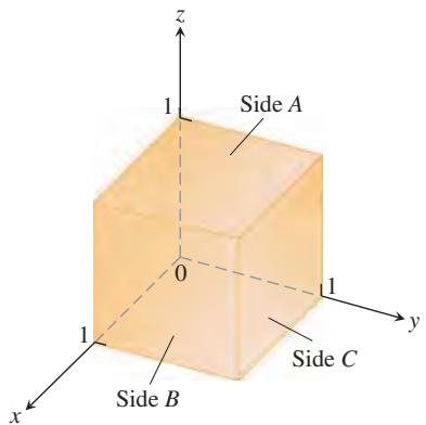
FIGURE 15.50 The cube in Example 2.
Solution We integrate xyz over each of the six sides and add the results. Since xyz = 0 on the sides that lie in the coordinate planes, the integral over the surface of the cube reduces to
Side A is the surface
and
Symmetry tells us that the integrals of xyz over sides B and C are also 1/4. Hence,
EXAMPLE 3 Integrate
Solution The surface is displayed in Figure 15.46, and in Example 6 of Section 15.5 we found the parametrization
where v represents the angle of rotation from the xz-plane about the z-axis. Substituting this parametrization into the expression for G gives
The surface area differential for the parametrization was found to be (Example 6, Section 15.5)
These calculations give the surface integral
EXAMPLE 4 Evaluate
FIGURE 15.51 The surface S in Example 4.
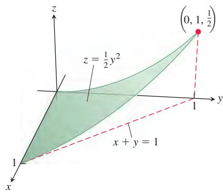
Solution The function G on the surface S is given by
With
and
(a)
(b)
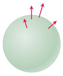
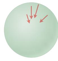
FIGURE 15.52 (a) An outward-pointing vector field and (b) an inward-pointing vector field give the two possible orientations of a sphere.
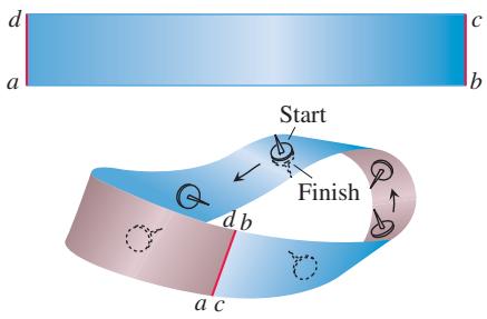
FIGURE 15.53 To make a Möbius band, take a rectangular strip of paper abcd, give the end bc a single twist, and paste the ends of the strip together to match a with c and b with d. The Möbius band is a nonorientable, or one-sided, surface.
Orientation of a Surface
A curve C with a parametrization
To specify an orientation on a surface in space S, we do something similar, but this time we specify a normal vector at each point on the surface. A parametrization of a surface
Each point on the sphere in Figure 15.52 has one normal vector pointing inward, toward the center of the sphere, and another opposite normal vector pointing outward. We specify one of two possible orientations for the sphere by choosing either the inward vector at each point, or alternatively the outward vector at each point.
When we can choose a continuous field of unit normal vectors
A surface together with its normal field n, or, equivalently, a surface with a consistent choice of sides, is called an oriented surface. The vector n at any point gives the positive direction or positively oriented side at that point (Figure 15.52). Not all surfaces can be oriented. The Möbius band in Figure 15.53 is an example of a surface that is not orientable. No matter how you try to construct a continuous unit normal vector field (shown as the shafts of thumbtacks in the figure), starting at one point and moving the vector continuously around the surface in the manner shown will return it to the starting point, but pointing in the opposite direction. No choice of a vectors can give a continuous normal vector field on the Möbius band, so the Möbius band is not orientable.
Surface Integrals of Vector Fields
In Section 15.2 we defined the line integral of a vector field along a path
DEFINITION Let F be a vector field in three-dimensional space with continuous components defined over a smooth surface S having a chosen field of normal unit vectors n orienting S. Then the surface integral of F over S is
∬ 𝑆 𝐅 ⋅ 𝐧 𝑑 𝜎 . ( 5 )
This integral is also called the flux of the vector field F across S.
If F is the velocity field of a three-dimensional fluid flow, then the flux of F across S is the net rate at which fluid is crossing S per unit time in the chosen positive direction n defined by the orientation of S. Fluid flows are discussed in more detail in Section 15.7.
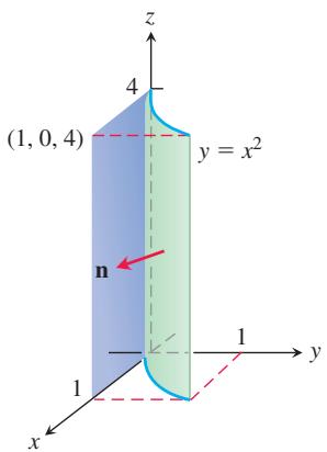
FIGURE 15.54 Finding the flux through the surface of a parabolic cylinder (Example 5).
Computing a Surface Integral for a Parametrized Surface
EXAMPLE 5 Find the flux of
Flux Across a Parametrized Surface
Flux = ±∫∫_R F · (r_u × r_v) du dv
Solution On the surface we have x = x,
can be used to find unit normal vectors to the surface,
We can equally well choose the unit normal vectors
On the surface we have
Thus,
The flux of F outward through the surface is
There is a simple formula for the flux of F across a parametrized surface
and
it follows that
The other choice of unit normal vector, -n, would add a negative sign to this formula. The choice of n or -n depends on the direction in which we choose to measure the flux across the surface.
This integral for flux simplifies the computation in Example 5 by eliminating the need to compute the canceled factor
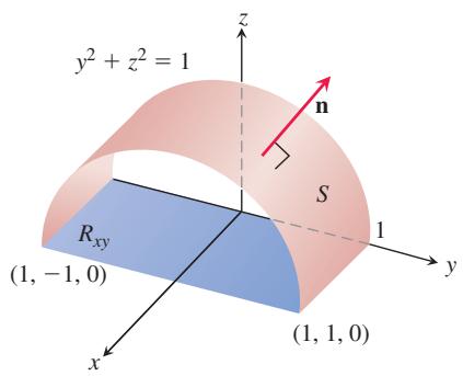
FIGURE 15.55 Calculating the flux of a vector field through the surface S. The area of the shadow region
we obtain directly
in Example 5.
Computing a Surface Integral for a Level Surface
If S is part of a level surface
depending on which one gives the preferred direction. The corresponding flux is
EXAMPLE 6 Find the flux of
Solution The normal field on S (Figure 15.55) in the specified direction may be calculated from the gradient of
With
We can drop the absolute value bars because
The value of
The surface projects onto the shadow region
Moments and Masses of Thin Shells
Thin shells of material like bowls, metal drums, and domes are modeled with surfaces. Their moments and masses are calculated with the formulas in Table 15.3. The derivations are similar to those in Section 6.6. The formulas resemble those for line integrals in Table 15.1, Section 15.1.
TABLE 15.3 Mass and moment formulas for very thin shells
Mass:
First moments about the coordinate planes:
Coordinates of center of mass:
Moments of inertia about coordinate axes:
FIGURE 15.56 The center of mass of a thin hemispherical shell of constant density lies on the axis of symmetry halfway from the base to the top (Example 7).
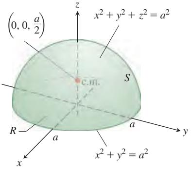
EXAMPLE 7 Find the center of mass of a thin hemispherical shell of radius a and constant density
Solution We model the shell with the hemisphere
(Figure 15.56). The symmetry of the surface about the
The mass of the shell is
To evaluate the integral for
Then
The shell’s center of mass is the point
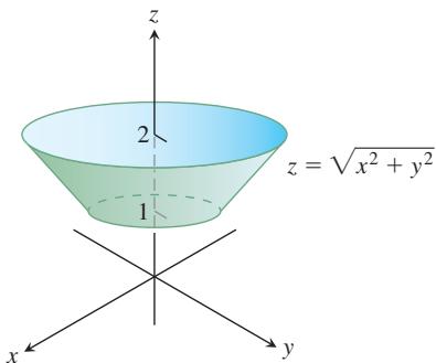
and
FIGURE 15.57 The cone frustum formed when the cone
EXAMPLE 8 Find the center of mass of a thin shell of density
Solution Since the surface and the density function
Therefore,
The shell’s center of mass is the point
EXERCISES 15.6
Surface Integrals of Scalar Functions
In Exercises 1–8, integrate the given function over the given surface.
-
Parabolic cylinder
𝐺 ( 𝑥 , 𝑦 , 𝑧 ) = 𝑥 𝑦 = 𝑥 2 0 ≤ 𝑥 ≤ 2 0 ≤ 𝑧 ≤ 3 -
Circular cylinder
𝐺 ( 𝑥 , 𝑦 , 𝑧 ) = 𝑧 𝑦 2 + 𝑧 2 = 4 , 𝑧 ≥ 0 , 1 ≤ 𝑥 ≤ 4 -
Sphere
𝐺 ( 𝑥 , 𝑦 , 𝑧 ) = 𝑥 2 𝑥 2 + 𝑦 2 + 𝑧 2 = 1 -
Hemisphere
𝐺 ( 𝑥 , 𝑦 , 𝑧 ) = 𝑧 2 𝑥 2 + 𝑦 2 + 𝑧 2 = 𝑎 2 𝑧 ≥ 0 -
Portion of plane
𝐹 ( 𝑥 , 𝑦 , 𝑧 ) = 𝑧 𝑥 + 𝑦 + 𝑧 = 4 0 ≤ 𝑥 ≤ 1 0 ≤ 𝑦 ≤ 1 -
Cone
𝐹 ( 𝑥 , 𝑦 , 𝑧 ) = 𝑧 − 𝑥 𝑧 = √ 𝑥 2 + 𝑦 2 0 ≤ 𝑧 ≤ 1 -
Parabolic dome
𝐻 ( 𝑥 , 𝑦 , 𝑧 ) = 𝑥 2 √ 5 − 4 𝑧 𝑧 = 1 − 𝑥 2 − 𝑦 2 𝑧 ≥ 0 -
Spherical cap
𝐻 ( 𝑥 , 𝑦 , 𝑧 ) = 𝑦 𝑧 𝑥 2 + 𝑦 2 + 𝑧 2 = 4 𝑧 = √ 𝑥 2 + 𝑦 2 -
Integrate
𝐺 ( 𝑥 , 𝑦 , 𝑧 ) = 𝑥 + 𝑦 + 𝑧 𝑥 = 𝑎 𝑦 = 𝑎 𝑧 = 𝑎 -
Integrate
𝐺 ( 𝑥 , 𝑦 , 𝑧 ) = 𝑦 + 𝑧 𝑦 + 𝑧 = 1 -
Integrate
𝐺 ( 𝑥 , 𝑦 , 𝑧 ) = 𝑥 𝑦 𝑧 -
Integrate
𝐺 ( 𝑥 , 𝑦 , 𝑧 ) = 𝑥 𝑦 𝑧 𝑥 = ± 𝑎 𝑦 = ± 𝑏 𝑧 = ± 𝑐 -
Integrate
𝐺 ( 𝑥 , 𝑦 , 𝑧 ) = 𝑥 + 𝑦 + 𝑧 2 𝑥 + 2 𝑦 + 𝑧 = 2 -
Integrate
𝐺 ( 𝑥 , 𝑦 , 𝑧 ) = 𝑥 √ 𝑦 2 + 4 𝑦 2 + 4 𝑧 = 1 6 𝑥 = 0 , 𝑥 = 1 𝑧 = 0 -
Integrate
𝐺 ( 𝑥 , 𝑦 , 𝑧 ) = 𝑧 − 𝑥 𝑧 = 𝑥 + 𝑦 2 ( 0 , 0 , 0 ) ( 1 , 1 , 0 ) ( 0 , 1 , 0 )
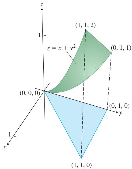
- Integrate
𝐺 ( 𝑥 , 𝑦 , 𝑧 ) = 𝑥
- Integrate
𝐺 ( 𝑥 , 𝑦 , 𝑧 ) = 𝑥 𝑦 𝑧 ( 1 , 0 , 0 ) ( 0 , 2 , 0 ) ( 0 , 1 , 1 )
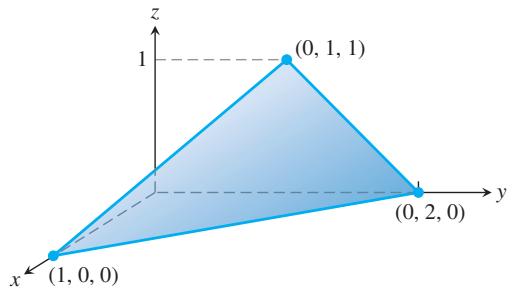
- Integrate
𝐺 ( 𝑥 , 𝑦 , 𝑧 ) = 𝑥 − 𝑦 − 𝑧 𝑥 + 𝑦 = 1 𝑧 = 0 𝑧 = 1
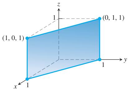
Finding Flux or Surface Integrals of Vector Fields
In Exercises 19–28, use a parametrization to find the flux
-
Parabolic cylinder
𝐹 = 𝑧 2 𝑖 + 𝑥 𝑗 − 3 𝑧 𝑘 𝑧 = 4 − 𝑦 2 -
Parabolic cylinder
𝐹 = 𝑥 2 𝑗 − 𝑥 𝑧 𝑘 𝑦 = 𝑥 2 , − 1 ≤ 𝑥 ≤ 1 -
Sphere
𝐅 = 𝑧 𝐤 𝑥 2 + 𝑦 2 + 𝑧 2 = 𝑎 2 -
Sphere
𝐹 = 𝑥 𝐢 + 𝑦 𝐣 + 𝑧 𝐤 𝑥 2 + 𝑦 2 + 𝑧 2 = 𝑎 2 -
Plane
𝐅 = 2 𝑥 𝑦 𝐢 + 2 𝑦 𝑧 𝐣 + 2 𝑥 𝑧 𝐤 𝑥 + 𝑦 + 𝑧 = 2 𝑎 0 ≤ 𝑥 ≤ 𝑎 0 ≤ 𝑦 ≤ 𝑎 -
Cylinder
𝐅 = 𝑥 𝐢 + 𝑦 𝐣 + 𝑧 𝐤 𝑥 2 + 𝑦 2 = 1 𝑧 = 0 𝑧 = 𝑎 𝑧 -
Cone
𝐹 = 𝑥 𝑦 𝐢 − 𝑧 𝐤 𝑧 = √ 𝑥 2 + 𝑦 2 0 ≤ 𝑧 ≤ 1 -
Cone
𝐹 = 𝑦 2 𝑖 + 𝑥 𝑧 𝑗 − 𝑘 𝑧 = 2 √ 𝑥 2 + 𝑦 2 0 ≤ 𝑧 ≤ 2 -
Cone frustum
𝐹 = − 𝑥 𝑖 − 𝑦 𝑗 + 𝑧 2 𝑘 𝑧 = √ 𝑥 2 + 𝑦 2 -
Paraboloid
𝐹 = 4 𝑥 𝑖 + 4 𝑦 𝑗 + 2 𝑘 𝑧 = 𝑥 2 + 𝑦 2
In Exercises 29 and 30, find the surface integral of the field F over the portion of the given surface in the specified direction.
-
𝐅 ( 𝑥 , 𝑦 , 𝑧 ) = − 𝐢 + 2 𝐣 + 3 𝐤 𝑧 = 0 0 ≤ 𝑥 ≤ 2 0 ≤ 𝑦 ≤ 3 𝐤 -
𝐅 ( 𝑥 , 𝑦 , 𝑧 ) = 𝑦 𝑥 2 𝐢 − 2 𝐣 + 𝑥 𝑧 𝐤 𝑦 = 0 , − 1 ≤ 𝑥 ≤ 2 , 2 ≤ 𝑧 ≤ 7 , − 𝐣
In Exercises 31–36, use Equation (7) to find the surface integral of the field F over the portion of the sphere
-
𝐅 ( 𝑥 , 𝑦 , 𝑧 ) = 𝑧 𝐤 -
𝐅 ( 𝑥 , 𝑦 , 𝑧 ) = − 𝑦 𝐢 + 𝑥 𝐣 -
𝐅 ( 𝑥 , 𝑦 , 𝑧 ) = 𝑦 𝐢 − 𝑥 𝐣 + 𝐤 -
𝐅 ( 𝑥 , 𝑦 , 𝑧 ) = 𝑧 𝑥 𝐢 + 𝑧 𝑦 𝐣 + 𝑧 2 𝐤 -
𝐅 ( 𝑥 , 𝑦 , 𝑧 ) = 𝑥 𝐢 + 𝑦 𝐣 + 𝑧 𝐤 -
𝐅 ( 𝑥 , 𝑦 , 𝑧 ) = 𝑥 𝐢 + 𝑦 𝐣 + 𝑧 𝐤 √ 𝑥 2 + 𝑦 2 + 𝑧 2 -
Find the flux of the field
𝐅 ( 𝑥 , 𝑦 , 𝑧 ) = 𝑧 2 𝐢 + 𝑥 𝐣 − 3 𝑧 𝐤 𝑧 = 4 − 𝑦 2 𝑥 = 0 𝑥 = 1 𝑧 = 0 𝑥 -
Find the flux of the field
𝐅 ( 𝑥 , 𝑦 , 𝑧 ) = 4 𝑥 𝐢 + 4 𝑦 𝐣 + 2 𝐤 𝑧 = 𝑥 2 + 𝑦 2 -
Let S be the portion of the cylinder
𝑦 = 𝑒 𝑥 𝑅 𝑦 𝑧 : 1 ≤ 𝑦 ≤ 2 , 0 ≤ 𝑧 ≤ 1 𝐅 ( 𝑥 , 𝑦 , 𝑧 ) = − 2 𝐢 + 2 𝑦 𝐣 + 𝑧 𝐤
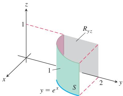
-
Let S be the portion of the cylinder
𝑦 = l n 𝑥 𝑅 𝑥 𝑧 : 1 ≤ 𝑥 ≤ 𝑒 , 0 ≤ 𝑧 ≤ 1 𝐹 = 2 𝑦 𝑗 + 𝑧 𝑘 -
Find the outward flux of the field
𝐹 = 2 𝑥 𝑦 𝑖 + 2 𝑦 𝑧 𝑗 + 2 𝑥 𝑧 𝑘 -
Find the outward flux of the field
𝐹 = 𝑥 𝑧 𝑖 + 𝑦 𝑧 𝑗 + 𝑘 𝑥 2 + 𝑦 2 + 𝑧 2 ≤ 2 5
Moments and Masses
-
Centroid Find the centroid of the portion of the sphere
𝑥 2 + 𝑦 2 + 𝑧 2 = 𝑎 2 -
Centroid Find the centroid of the surface cut from the cylinder
𝑦 2 + 𝑧 2 = 9 𝑧 ≥ 0 -
Thin shell of constant density Find the center of mass and the moment of inertia about the z-axis of a thin shell of constant density
𝛿 𝑥 2 + 𝑦 2 − 𝑧 2 = 0
15.7 Stokes’ Theorem
- Conical surface of constant density Find the moment of inertia about the z-axis of a thin shell of constant density
𝛿 4 𝑥 2 + 4 𝑦 2 − 𝑧 2 = 0 𝑧 ≥ 0 𝑥 2 + 𝑦 2 = 2 𝑥
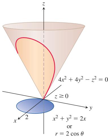
-
Spherical shells Find the moment of inertia about a diameter of a thin spherical shell of radius a and constant density
𝛿 -
Conical Surface Find the centroid of the lateral surface of a solid cone of base radius
𝑎 ℎ -
A surface S lies on the plane
2 𝑥 + 3 𝑦 + 6 𝑧 = 1 2 ( 0 , 0 ) ( 1 , 0 ) ( 0 , 2 ) ( 1 , 2 ) ( 𝑥 , 𝑦 , 𝑧 ) 𝛿 ( 𝑥 , 𝑦 , 𝑧 ) = 4 𝑥 𝑦 + 6 𝑧 m g / c m 2 -
A surface S lies on the paraboloid
𝑧 = 1 2 𝑥 2 + 1 2 𝑦 2 ( 0 , 0 ) ( 2 , 0 ) ( 2 , 4 ) ( 𝑥 , 𝑦 , 𝑧 ) 𝛿 ( 𝑥 , 𝑦 , 𝑧 ) = 9 𝑥 𝑦 𝑔 / 𝑐 𝑚 2
To calculate the counterclockwise circulation of a two-dimensional vector field
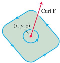
FIGURE 15.58 The circulation vector at a point
∇ is the symbol “del.”
The Curl Vector Field
Suppose that
This information is a consequence of Stokes’ Theorem, the generalization to space of the circulation-curl form of Green’s Theorem.
Notice that
The symbol
We often use this cross product notation to write the curl symbolically as “del cross F.”
EXAMPLE 1 Find the curl of
Solution We use Equation (3) and the determinant form for the cross product, which gives,
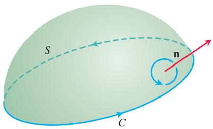
FIGURE 15.59 The orientation of the bounding curve C gives it a right-hand relation to the normal field n. If the thumb of a right hand points along n, the fingers curl in the direction of C.
As we will see, the operator
In this setting it is read sometimes as “del f” and sometimes as “grad f.”
Stokes’ Theorem
Stokes’ Theorem generalizes Green’s Theorem to three dimensions. The circulation-curl form of Green’s Theorem relates the counterclockwise circulation of a vector field around a simple closed curve
THEOREM 6—Stokes’ Theorem
Let
Notice from Equation (4) that if two different oriented surfaces
Both curl integrals equal the counterclockwise circulation integral on the left side of Equation (4) as long as the unit normal vectors
If
Under these conditions, Stokes’ equation becomes
which is the circulation-curl form of the equation in Green’s Theorem. Conversely, by reversing these steps we can rewrite the circulation-curl form of Green’s Theorem for two-dimensional fields in del notation as
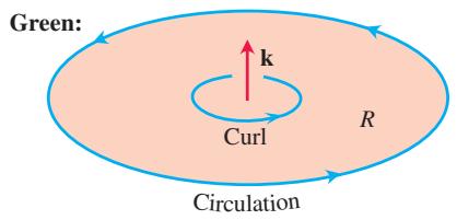
(5)
FIGURE 15.60 When applied to curves and surfaces in the plane, Stokes’ Theorem gives the circulation-curl version of Green’s Theorem. But Stokes’ Theorem also applies more generally, to curves and surfaces not lying in the plane.
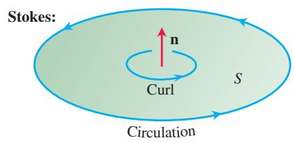
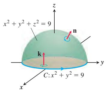
FIGURE 15.61 A hemisphere and a disk, each with boundary C (Examples 2 and 3).
See Figure 15.60.
EXAMPLE 2 Evaluate both sides of Equation (4) for the hemisphere
Solution The hemisphere looks much like the surface in Figure 15.59 with the bounding circle C in the xy-plane (see Figure 15.61). We calculate the counterclockwise circulation around C (as viewed from above) using the parametrization
When evaluating the right side of Equation (4), we choose the orientation of the unit normal vector so that it points away from the origin, giving it a right-hand relation to the prescribed orientation of the curve C (see Figure 15.61). We have
and
The circulation around the circle equals the integral of the curl over the hemisphere, as it should from Stokes’ Theorem.
The surface integral in Stokes’ Theorem can be computed using any surface having boundary curve
EXAMPLE 3 Calculate the circulation around the bounding circle C in Example 2, using the disk of radius 3 centered at the origin in the xy-plane as the surface S (instead of the hemisphere). See Figure 15.61.
Solution As in Example 2,
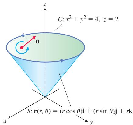
FIGURE 15.62 The curve C and cone S in Example 4.
and
a simpler calculation than before.
EXAMPLE 4 Find the circulation of the field
Solution Stokes’ Theorem enables us to find the circulation by integrating over the surface of the cone. Traversing
We parametrize the cone as
We then have
Accordingly,
and the circulation is
EXAMPLE 5 The cone used in Example 4 is not the easiest surface to use for calculating the circulation around the bounding circle C lying in the plane z = 2. If instead we use the flat disk of radius 2 centered on the z-axis and lying in the plane z = 2, then the normal vector to the surface S is n = k (chosen to give a counterclockwise direction for the curve C). Just as in the computation for Example 4, we still have
This result agrees with the circulation value found in Example 4.
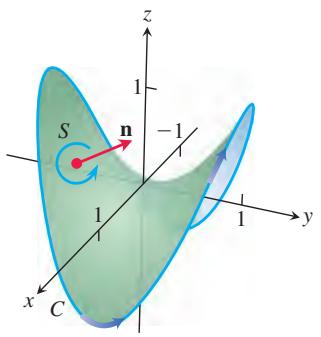
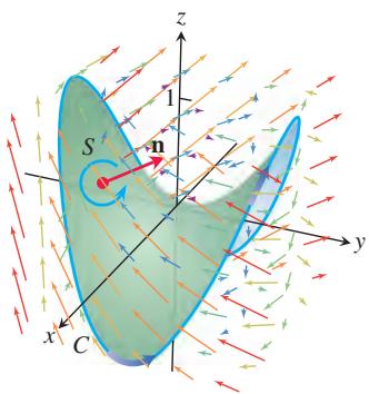
FIGURE 15.63 The surface and vector field for Example 6.
EXAMPLE 6 Find a parametrization for the surface S formed by the part of the hyperbolic paraboloid
Solution As the unit circle is traversed in the xy-plane, the z-coordinate of the surface with the curve C as boundary is given by
with
Along the curve
The counterclockwise circulation along C is the value of the line integral
We now compute the same quantity by integrating
We next compute
and
Note that the k-component is always nonnegative. Therefore, we take
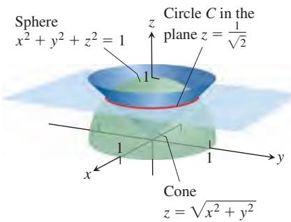
FIGURE 15.64 Circulation curve C in Example 7.
We now obtain
So the surface integral of
EXAMPLE 7 Calculate the circulation of the vector field
along the curve of intersection of the sphere
Solution The sphere and cone intersect when
so that
Paddle Wheel Interpretation of ∇ × 𝐅
Suppose that F is the velocity field of a fluid moving in a region R in space containing the closed curve C. Then
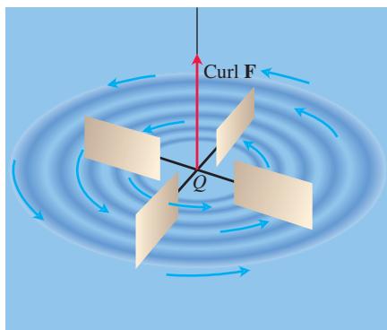
FIGURE 15.65 A small paddle wheel in a fluid spins fastest at point Q when its axle points in the direction of curl F.
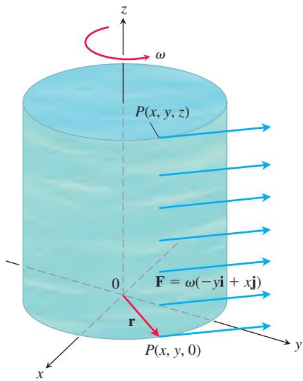
FIGURE 15.66 A steady rotational flow parallel to the xy-plane, with constant angular velocity ω in the positive (counterclockwise) direction (Example 8).
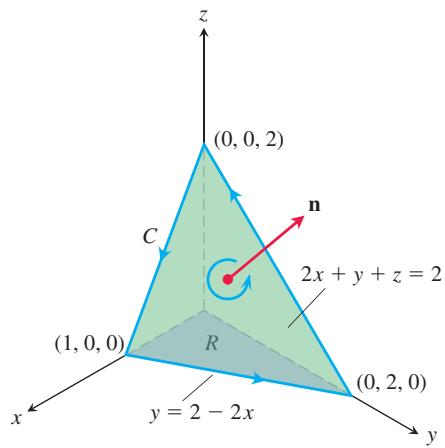
FIGURE 15.67 The planar surface in Example 9.
is the circulation of the fluid around C. By Stokes’ Theorem, the circulation is equal to the flux of
Suppose we fix a point Q in the region R and a direction u at Q. Take C to be a circle of radius
If we apply Stokes’ Theorem and replace the surface integral by a line integral over C, we get
The left-hand side of Equation (6) has its maximum value when u is the direction of
which is the circulation around C divided by the area of the disk (circulation density). Suppose that a small paddle wheel of radius
EXAMPLE 8 A fluid of constant density rotates around the z-axis with velocity
Solution With
and therefore
Solving this last equation for
which is consistent with Equation (6) when
EXAMPLE 9 Use Stokes’ Theorem to evaluate
Solution The plane is the level surface
is consistent with the counterclockwise motion around C. To apply Stokes’ Theorem, we find
On the plane, z equals
and
FIGURE 15.68 The portion of the elliptic paraboloid in Example 10, showing its curve of intersection C with the plane
The surface area differential is
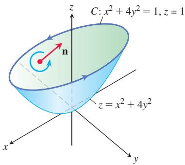
The circulation is
EXAMPLE 10 Let the surface S be the elliptic paraboloid
Solution We use Stokes’ Theorem to calculate the curl integral by finding the equivalent counterclockwise circulation of F around the curve of intersection C of the paraboloid
To compute the circulation integral
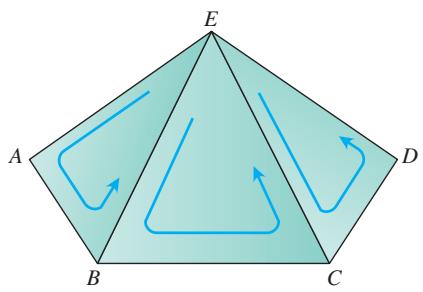
(a)
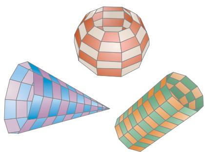
(b)
FIGURE 15.69 (a) Part of a polyhedral surface. (b) Other polyhedral surfaces.
and
Then
Therefore, by Stokes’ Theorem the flux of the curl across S in the direction n for the field F is
Proof Outline of Stokes’ Theorem for Polyhedral Surfaces
Let S be a polyhedral surface consisting of a finite number of plane regions or faces. (See Figure 15.69 for examples.) We apply Green’s Theorem to each separate face of S. There are two types of faces:
-
Those that are surrounded on all sides by other faces.
-
Those that have one or more edges that are not adjacent to other faces.
The boundary of S consists of those edges of the type 2 faces that are not adjacent to other faces. In Figure 15.69a, the triangles EAB, BCE, and CDE represent a part of S, with ABCD part of the boundary of the surface, boundary(S). Although Green’s Theorem was stated for curves in the xy-plane, a generalized form applies to curves that lie in a plane in space. In the generalized form, the theorem asserts that the line integral of F around the curve enclosing the plane region R normal to n equals the double integral of (curl F n ) ⋅ over R. Applying this generalized form to the three triangles of Figure 15.69a in turn, and adding the results, gives
The three line integrals on the left-hand side of Equation (7) combine into a single line integral taken around the periphery ABCDE because the integrals along interior segments cancel in pairs. For example, the integral along segment BE in triangle ABE is opposite in sign to the integral along the same segment in triangle EBC. The same holds for segment CE. Hence, Equation (7) reduces to
When we apply Green’s Theorem to all the faces and add the results, we get
(b)
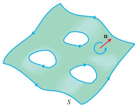
FIGURE 15.70 Stokes’ Theorem also holds for oriented surfaces with holes. Consistent with the orientation of S, the outer curve is traversed counterclockwise around n, and the inner curves surrounding the holes are traversed clockwise.
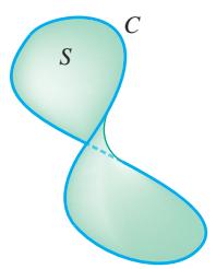
(a)
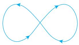
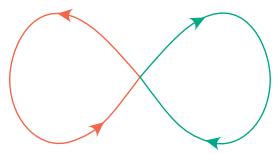
FIGURE 15.71 (a) In a simply connected open region in space, a simple closed curve C is the boundary of a smooth surface S. (b) Smooth curves that cross themselves can be divided into loops to which Stokes’ Theorem applies.
This is Stokes’ Theorem for the polyhedral surface S in Figure 15.69a. More general polyhedral surfaces are shown in Figure 15.69b, and the proof can be extended to them. General smooth surfaces can be obtained as limits of polyhedral surfaces.
Stokes’ Theorem for Surfaces with Holes
Stokes’ Theorem holds for an oriented surface S that has one or more holes (Figure 15.70). The surface integral over S of the normal component of
An Important Identity
The following identity arises frequently in mathematics and the physical sciences.
Forces arising in the study of electromagnetism and gravity are often associated with a potential function
If the second partial derivatives are continuous, the mixed second derivatives in parentheses are equal (Theorem 2, Section 13.3) and the vector is zero.
Conservative Fields and Stokes’ Theorem
In Section 15.3, we found that a field F being conservative in an open region D in space is equivalent to the integral of F around every closed loop in D being zero. This, in turn, is equivalent in simply connected open regions to saying that
THEOREM 7— Curl F 0= Related to the Closed-Loop Property If
Sketch of a Proof Theorem 7 can be proved in two steps. The first step is for simple closed curves (loops that do not cross themselves), like the one in Figure 15.71a. A theorem from topology, a branch of advanced mathematics, states that every smooth simple closed curve C in a simply connected open region D is the boundary of a smooth two-sided surface S that also lies in D. Hence, by Stokes’ Theorem,
The second step is for curves that cross themselves, like the one in Figure 15.71b. The idea is to break these into simple loops spanned by orientable surfaces, apply Stokes Theorem one loop at a time, and add the results.
The following diagram summarizes the results for conservative fields defined on connected, simply connected open regions. For such regions, the four statements are equivalent to each other.
Exercises 15.7
In Exercises 1–6, find the curl of each vector field F.
𝐅 = ( 𝑥 + 𝑦 − 𝑧 ) 𝐢 + ( 2 𝑥 − 𝑦 + 3 𝑧 ) 𝐣 + ( 3 𝑥 + 2 𝑦 + 𝑧 ) 𝐤
Using Stokes’ Theorem to Find Line Integrals
In Exercises 7–12, use the surface integral in Stokes’ Theorem to calculate the circulation of the field F around the curve C in the indicated direction.
C: The ellipse
C: The circle
C: The boundary of the triangle cut from the plane
C: The boundary of the triangle cut from the plane x
𝐅 = ( 𝑦 2 + 𝑧 2 ) 𝐢 + ( 𝑥 2 + 𝑦 2 ) 𝐣 + ( 𝑥 2 + 𝑦 2 ) 𝐤
C: The square bounded by the lines
C: The intersection of the cylinder
Integral of the Curl Vector Field
- Let n be the unit normal in the direction away from the origin of the elliptic shell
and let
Find the value of
(Hint: One parametrization of the ellipse at the base of the shell is x = = ≤ ≤3 cos , 2 sin , 0 2 .)t y t t π
- Let n be the unit normal in the direction away from the origin of the parabolic shell
and let
Find the value of
-
Let S be the cylinder
𝑥 2 + 𝑦 2 = 𝑎 2 , 0 ≤ 𝑧 ≤ ℎ , 𝑥 2 + 𝑦 2 ≤ 𝑎 2 , 𝑧 = ℎ 𝐅 = − 𝑦 𝐢 + 𝑥 𝐣 + 𝑥 2 𝐤 ∇ × 𝐅 -
Evaluate
where S is the hemisphere
- Suppose
𝐅 = ∇ × 𝐀
Determine the flux of F through the hemisphere
- Repeat Exercise 17 for the flux of F across the entire unit sphere.
Stokes’ Theorem for Parametrized Surfaces
In Exercises 19–24, use the surface integral in Stokes’ Theorem to calculate the flux of the curl of the field F across the surface S.
𝐅 = 2 𝑧 𝐢 + 3 𝑥 𝐣 + 5 𝑦 𝐤
in the direction away from the origin.
𝐅 = ( 𝑦 − 𝑧 ) 𝐢 + ( 𝑧 − 𝑥 ) 𝐣 + ( 𝑥 + 𝑧 ) 𝐤
in the direction away from the origin.
𝐅 = 𝑥 2 𝑦 𝐢 + 2 𝑦 3 𝑧 𝐣 + 3 𝑧 𝐤
in the direction away from the z-axis.
𝐅 = ( 𝑥 − 𝑦 ) 𝐢 + ( 𝑦 − 𝑧 ) 𝐣 + ( 𝑧 − 𝑥 ) 𝐤
in the direction away from the z-axis.
𝐅 = 3 𝑦 𝐢 + ( 5 − 2 𝑥 ) 𝐣 + ( 𝑧 2 − 2 ) 𝐤
in the direction away from the origin.
𝐅 = 𝑦 2 𝐢 + 𝑧 2 𝐣 + 𝑥 𝐤
φ θ φ θ φ θ φ( ) ( ) ( ) ( )= + +S: , 2 sin cos 2 sin sin 2 cos , r i j k
in the direction away from the origin.
Theory and Examples
- Let C be the smooth curve
𝐫 ( 𝑡 ) = ( 2 c o s 𝑡 ) 𝐢 + ( 2 s i n 𝑡 ) 𝐣 + ( 3 − 2 c o s 3 𝑡 ) 𝐤 𝑥 2 + 𝑦 2 = 4 𝑧 ≥ 0 , 𝐅 = 𝑦 𝐢 − 𝑥 𝐣 + 𝑥 2 𝐤 .
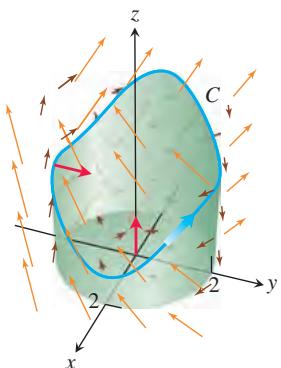
-
Verify Stokes’ Theorem for the vector field
𝐅 = 2 𝑥 𝑦 𝐢 + 𝑥 𝐣 𝛼 + 𝛼 ( 𝑦 + 𝑧 ) 𝐤 𝑧 = 4 − 𝑥 2 − 𝑦 2 , 𝑧 ≥ 0 -
Zero circulation Use Equation (8) and Stokes’ Theorem to show that the circulations of the following fields around the boundary of any smooth orientable surface in space are zero.
- Zero circulation Let
𝑓 ( 𝑥 , 𝑦 , 𝑧 ) = ( 𝑥 2 + 𝑦 2 + 𝑧 2 ) − 1 / 2 𝐅 = ∇ 𝑓 𝑥 2 + 𝑦 2 = 𝑎 2 𝐫 = ( 𝑎 c o s 𝑡 ) 𝐢 + ( 𝑎 s i n 𝑡 ) 𝐣 , 0 ≤ 𝑡 ≤ 2 𝜋
b. by applying Stokes’ Theorem.
- Let C be a simple closed smooth curve in the plane
2 𝑥 + 2 𝑦 + 𝑧 = 2 ,
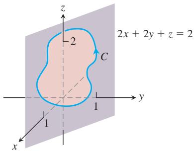
depends only on the area of the region enclosed by C and not on the position or shape of C.
-
Show that if
𝐅 = 𝑥 𝐢 + 𝑦 𝐣 + 𝑧 𝐤 ∇ × 𝐅 = 𝟎 -
Find a vector field with twice-differentiable components whose curl is xi
+ 𝑦 𝐣 + 𝑧 𝐤 -
Does Stokes’ Theorem say anything special about circulation in a field whose curl is zero? Give reasons for your answer.
-
Let R be a region in the xy-plane that is bounded by a piecewise smooth simple closed curve C, and suppose that the density is
𝛿 = 1 𝐼 𝑥 𝐼 Δ v .
where
- Zero curl, yet the field is not conservative Show that the curl of
is zero but that
is not zero if C is the circle
15.8 The Divergence Theorem and a Unified Theory
The divergence form of Green’s Theorem in the plane states that the net outward flux of a vector field across a simple closed curve can be calculated by integrating the divergence of the field over the region enclosed by the curve. The corresponding theorem in three dimensions, called the Divergence Theorem, states that the net outward flux of a vector field across a closed surface in space can be calculated by integrating the divergence of the field over the solid region enclosed by the surface. In this section we prove the Divergence Theorem and show how it simplifies the calculation of flux, which is the integral of the field over the closed oriented surface. We also derive Gauss’s law for flux in an electric field and the continuity equation of hydrodynamics. Finally, we summarize the chapter’s vector integral theorems in a single unifying principle generalizing the Fundamental Theorem of Calculus.
Divergence in Three Dimensions
The divergence of a vector field
The symbol “div
Div F has the same physical interpretation in three dimensions as it has in two. If F is the velocity field of a flowing gas, the value of div F at a point
EXAMPLE 1 The following vector fields represent the velocity of a gas flowing in space. Find the divergence of each vector field and interpret its physical meaning. Figure 15.72 displays the vector fields.
(a) Expansion:
(b) Compression:
(c) Rotation about the z-axis:
(d) Shearing along parallel horizontal planes:
Solution
(a) div
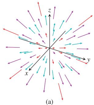
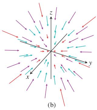
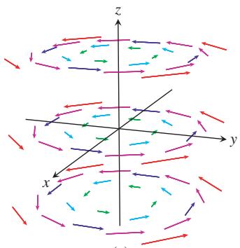
(c)
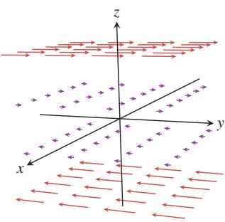
(d)
FIGURE 15.72 Velocity fields of a gas flowing in space (Example 1).
(b) div
(c) div
(d) div
Divergence Theorem
The Divergence Theorem says that under suitable conditions, the outward flux of a vector field across a closed surface equals the triple integral of the divergence of the field over the three-dimensional region enclosed by the surface.
THEOREM 8—Divergence Theorem
Let F be a vector field whose components have continuous first partial derivatives, and let S be a piecewise smooth oriented closed surface. The flux of F across S in the direction of the surface’s outward unit normal field n equals the triple integral of the divergence ∇ ⋅ F over the solid region D enclosed by the surface:
EXAMPLE 2 Evaluate both sides of Equation (2) for the expanding vector field
Solution The outer unit normal to S, calculated from the gradient of
It follows that
Therefore, the outward flux is
For the right-hand side of Equation (2), the divergence of F is
so we obtain the divergence integral,
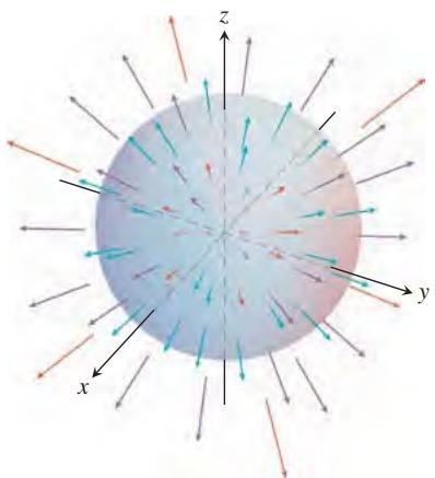
FIGURE 15.73 A uniformly expanding vector field and a sphere (Example 2).
Many vector fields of interest in applied science have zero divergence at each point. A common example is the velocity field of a circulating incompressible liquid, since it is neither expanding nor contracting. Other examples include constant vector fields
COROLLARY The outward flux across a piecewise smooth oriented closed surface S is zero for any vector field F having zero divergence at every point of the region enclosed by the surface.
EXAMPLE 3 Find the flux of
Solution Instead of calculating the flux as a sum of six separate integrals, one for each face of the cube, we can calculate the flux by integrating the divergence
over the cube’s interior:
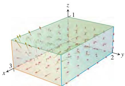
FIGURE 15.74 The integral of div F over this region equals the total flux across the six sides (Example 4).
EXAMPLE 4
(a) Calculate the flux of the vector field
out of the box-shaped region
(b) Integrate div F over this region and show that the result is the same value as in part (a), as asserted by the Divergence Theorem.
Solution
(a) The region D has six sides. We calculate the flux across each side in turn. Consider the top side in the plane z = 1, having outward normal n k = . The flux across this side is given by
The outward flux across the other sides is computed similarly, and the results are summarized in the following table.
| Side | Unit normal n | F · n | Flux across side |
| x = 0 | -i | 0 | |
| x = 3 | i | 18 | |
| y = 0 | -j | 0 | |
| y = 2 | j | 18 | |
| z = 0 | -k | 0 | |
| z = 1 | k |
The total outward flux is obtained by adding the terms for each of the six sides:
(b) We first compute the divergence of F, obtaining
The integral of the divergence of F over D is
As asserted by the Divergence Theorem, the integral of the divergence over D equals the outward flux across the boundary surface of D. ■
Divergence and the Curl
If F is a vector field on three-dimensional space, then the curl
THEOREM 9
Proof From the definitions of the divergence and curl, we have
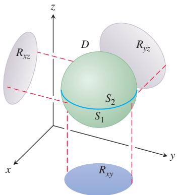
FIGURE 15.75 We prove the Divergence Theorem for the kind of threedimensional region shown here.
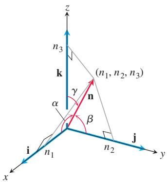
FIGURE 15.76 The components of n are the cosines of the angles α,
because the mixed second partial derivatives cancel by the Mixed Derivative Theorem in Section 13.3.
Theorem 9 has some interesting applications. If a vector field G = curl F, then the field G must have divergence 0. Saying this another way, if div
Proof of the Divergence Theorem for Special Regions
To prove the Divergence Theorem, we take the components of
with
The components of the unit normal vector
Thus the unit normal vector is given by
and
In component form, the Divergence Theorem states that
We prove the theorem by establishing the following three equations:
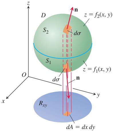
FIGURE 15.77 The region D enclosed by the surfaces
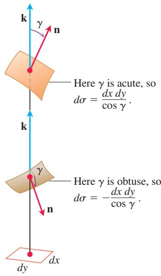
FIGURE 15.78 An enlarged view of the area patches in Figure 15.77. The relations dσ γ= ±dx dy cos come from Eq. (7) in Section 15.5 with
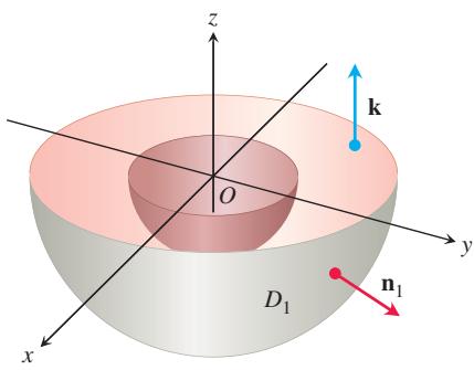
FIGURE 15.79 The lower half of the solid region between two concentric spheres.
Proof of Equation (5) We prove Equation (5) by converting the surface integral on the left to a double integral over the projection
See Figure 15.78. On
Therefore,
This proves Equation (5). The proofs for Equations (3) and (4) follow the same pattern; just permute
Divergence Theorem for Other Regions
The Divergence Theorem can be extended to regions that can be partitioned into a finite number of simple regions of the type just discussed and to regions that can be defined as limits of simpler regions in certain ways. For an example of one step in such a splitting process, suppose that
The unit normal
As we follow
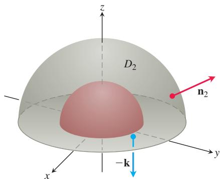
FIGURE 15.80 The upper half of the solid region between two concentric spheres.
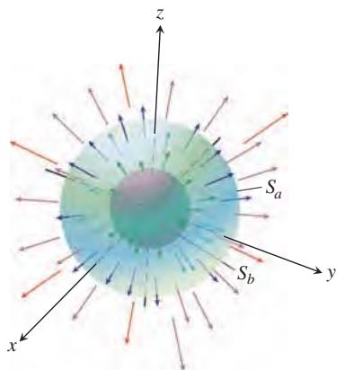
FIGURE 15.81 Two concentric spheres in an expanding vector field. The outer sphere
with D the region between the spheres, S the boundary of D consisting of two spheres, and n the unit normal to S directed outward from D.
EXAMPLE 5 Find the net outward flux of the field
across the boundary of the region D:
Solution The flux can be calculated by integrating
and
Similarly,
Hence,
So the net outward flux of F across the boundary of D is zero by the corollary to the Divergence Theorem. There is more to learn about this vector field F, though. The flux leaving D across the inner sphere
To find it, we evaluate the flux integral directly for an arbitrary sphere
Hence, on the sphere,
and
The outward flux of F in Equation (8) across any sphere centered at the origin is
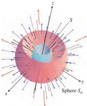
FIGURE 15.82 A sphere
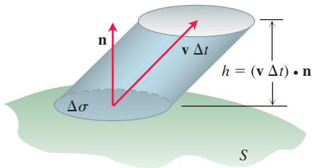
FIGURE 15.83 The fluid that flows upward through the patch
Gauss’s Law: One of the Four Great Laws of Electromagnetic Theory
In electromagnetic theory, the electric field created by a point charge q located at the origin is
where
The calculations in Example 5 show that the outward flux of E across any sphere centered at the origin is
when
So the flux of E across S in the direction away from the origin must be the same as the flux of E across
Continuity Equation of Hydrodynamics
Let D be a region in space bounded by a closed oriented surface
If the functions involved have continuous first partial derivatives, the equation evolves naturally from the Divergence Theorem, as we now demonstrate.
First, the integral
is the rate at which mass leaves D across S (leaves because n is the outer normal). To see why, consider a patch of area
The mass of this volume of fluid is about
so the rate at which mass is flowing out of D across the patch is about
This leads to the approximation
as an estimate of the average rate at which mass flows across S. Finally, letting
which for our particular flow is
Now let B be a solid sphere centered at a point Q in the flow. The average value of
It is a consequence of the continuity of the divergence that
The last term of the equation describes decrease in mass per unit volume.
Now let the radius of B approach zero while the center Q stays fixed. The left side of Equation (9) converges to
The continuity equation “explains” ∇ ⋅ F: The divergence of F at a point is the rate at which the density of the fluid is decreasing there. The Divergence Theorem
now says that the net decrease in density of the fluid in region D (divergence integral) is accounted for by the mass transported across the surface S (outward flux integral). So, the theorem is a statement about conservation of mass (Exercise 35).
Unifying the Integral Theorems
If we think of a two-dimensional field
Similarly,
With the equations of Green’s Theorem expressed in del notation, we can see their relationships to the equations in Stokes’ Theorem and the Divergence Theorem, all summarized here.
Green’s Theorem and Its Generalization to Three Dimensions
Tangential form of Green’s Theorem:
Stokes’ Theorem:
Normal form of Green’s Theorem:
Divergence Theorem:
Notice how Stokes’ Theorem generalizes the tangential (curl) form of Green’s Theorem from a flat surface in the plane to a surface in three-dimensional space. In each case, the surface integral of curl F over the interior of the oriented surface equals the circulation of F around the boundary.
Likewise, the Divergence Theorem generalizes the normal (flux) form of Green’s Theorem from a two-dimensional region in the plane to a three-dimensional region in space. In each case, the integral of ∇ ⋅ F over the interior of the region equals the total flux of the field across the boundary enclosing the region.
All these results can be thought of as forms of a single fundamental theorem. The Fundamental Theorem of Calculus in Section 5.4 says that if f(x) is differentiable on

FIGURE 15.84 The outward unit normals at the boundary of
If we let
The Fundamental Theorem now says that
The Fundamental Theorem of Calculus, the normal form of Green’s Theorem, and the Divergence Theorem all say that the integral of the differential operator ∇ ⋅ operating on a field F over a region equals the sum of the normal field components over the boundary enclosing the region. (Here we are interpreting the line integral in Green’s Theorem and the surface integral in the Divergence Theorem as “sums” over the boundary.)
Stokes’ Theorem and the tangential form of Green’s Theorem say that, when things are properly oriented, the surface integral of the differential operator
The beauty of these interpretations is the observance of a single unifying principle, which we can state as follows.
A Unifying Fundamental Theorem of Vector Integral Calculus
The integral of a differential operator acting on a field over a region equals the sum of the field components appropriate to the operator over the boundary of the region.
EXERCISES 15.8
Calculating Divergence
In Exercises 1–8, find the divergence of the field.
-
F = − + + + − + + − ( ) ( ) ( ) x y z x y z x y z i j k 2 3 2 2
-
𝐅 = ( 𝑥 l n 𝑦 ) 𝐢 + ( 𝑦 l n 𝑧 ) 𝐣 + ( 𝑧 l n 𝑥 ) 𝐤 -
𝐅 = 𝑦 𝑒 𝑥 𝑦 𝑧 𝐢 + 𝑧 𝑒 𝑥 𝑦 𝑧 𝐣 + 𝑥 𝑒 𝑥 𝑦 𝑧 𝐤 -
𝐅 = s i n ( 𝑥 𝑦 ) 𝐢 + c o s ( 𝑦 𝑧 ) 𝐣 + t a n ( 𝑥 𝑧 ) 𝐤 -
The spin field in Figure 15.13
-
The radial field in Figure 15.12
-
The gravitational field in Figure 15.9 and Exercise 38a in Section 15.3
-
The velocity field
𝐯 ( 𝑥 , 𝑦 , 𝑧 ) = ( 𝑎 2 − 𝑥 2 − 𝑦 2 )
Calculating Flux Using the Divergence Theorem
In Exercises 9–20, use the Divergence Theorem to find the outward flux of F across the boundary of the region D.
-
Cube
𝐅 = ( 𝑦 − 𝑥 ) 𝐢 + ( 𝑧 − 𝑦 ) 𝐣 + ( 𝑦 − 𝑥 ) 𝐤 𝑥 = ± 1 , 𝑦 = ± 1 , -
𝐅 = 𝑥 2 𝐢 + 𝑦 2 𝐣 + 𝑧 2 𝐤
a. Cube D: The cube cut from the first octant by the planes
c. Cylindrical can D: The region cut from the solid cylinder
- Cylinder and paraboloid
𝐅 = y 𝐢 + 𝑥 y 𝐣 − 𝑧 𝐤
D: The region inside the solid cylinder
-
Ball
𝐅 = 𝑥 2 𝐢 + 𝑥 𝑧 𝐣 + 3 𝑧 𝐤 𝑥 2 + 𝑦 2 + 𝑧 2 ≤ 4 -
Portion of bal
𝐅 = 𝑥 2 𝐢 − 2 𝑥 𝑦 𝐣 + 3 𝑥 𝑧 𝐤
D: The region cut from the first octant by the ball
-
Cylindrical can
𝐅 = ( 6 𝑥 2 + 2 𝑥 𝑦 ) 𝐢 + ( 2 𝑦 + 𝑥 2 𝑧 ) 𝐣 + 4 𝑥 2 𝑦 3 𝐤 𝑥 2 + 𝑦 2 = 4 -
Wedge
𝐅 = 2 𝑥 𝑧 𝐢 − 𝑥 𝑦 𝐣 − 𝑧 2 𝐤 𝑦 + 𝑧 = 4 𝑥 2 + 𝑦 2 = 1 6
-
Thick sphere
𝐅 = √ 𝑥 2 + 𝑦 2 + 𝑧 2 ( 𝑥 𝐢 + 𝑦 𝐣 + 𝑧 𝐤 ) 1 ≤ 𝑥 2 + 𝑦 2 + 𝑧 2 ≤ 2 -
Thick sphere
𝐅 = ( 𝑥 𝐢 + 𝑦 𝐣 + 𝑧 𝐤 ) / √ 𝑥 2 + 𝑦 2 + 𝑧 2 1 ≤ 𝑥 2 + 𝑦 2 + 𝑧 2 ≤ 4 -
Thick sphere
𝐅 = ( 5 𝑥 3 + 1 2 𝑥 𝑦 2 ) 𝐢 + ( 𝑦 3 + 𝑒 𝑦 s i n 𝑧 ) 𝐣 + ( 5 𝑧 3 + 𝑒 𝑦 c o s 𝑧 ) 𝐤 𝑥 2 + 𝑦 2 + 𝑧 2 = 1 𝑥 2 + 𝑦 2 + 𝑧 2 = 2 -
Thick cylinder
𝐅 = l n ( 𝑥 2 + 𝑦 2 ) 𝐢 − ( 2 𝑧 𝑥 a r c t a n 𝑦 𝑥 ) 𝐣 + 𝑧 √ 𝑥 2 + 𝑦 2 𝐤 1 ≤ 𝑥 2 + 𝑦 2 ≤ 2 , − 1 ≤ 𝑧 ≤ 2
Theory and Examples
- a. Show that the outward flux of the position vector field F = xi j k+ +y z through a smooth closed surface S is three times the volume of the region enclosed by the surface.
b. Let n be the outward unit normal vector field on S. Show that it is not possible for F to be orthogonal to n at every point of S.
- The base of the closed cubelike surface shown here is the unit square in the xy-plane. The four sides lie in the planes
𝑥 = 0 , 𝑥 = 1 , 𝑦 = 0 , a n d 𝑦 = 1 L e t 𝐅 = 𝑥 𝐢 − 2 𝑦 𝐣 + ( 𝑧 + 3 ) 𝐤 𝐵 i s − 3 .
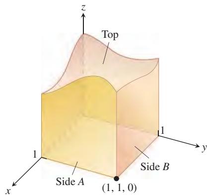
-
Let
𝐅 = ( 𝑦 c o s 2 𝑥 ) 𝐢 + ( 𝑦 2 s i n 2 𝑥 ) 𝐣 + ( 𝑥 2 𝑦 + 𝑧 ) 𝐤 𝐅 = ∇ × 𝐀 \ b o l d s y m b o l ? -
Outward flux of a gradient field Let S be the surface of the portion of the ball
𝑥 2 + 𝑦 2 + 𝑧 2 ≤ 𝑎 2 𝑓 ( 𝑥 , 𝑦 , 𝑧 ) = l n √ 𝑥 2 + 𝑦 2 + 𝑧 2
- Let F be a field whose components have continuous first partial derivatives throughout a portion of space containing a region D bounded by a smooth closed surface S.
. I f | 𝐅 | ≤ 1
Give reasons for your answer.
-
Maximum flux Among all rectangular boxes defined by the inequalities
0 ≤ 𝑥 ≤ 𝑎 , 0 ≤ 𝑦 ≤ 𝑏 , 0 ≤ 𝑧 ≤ 1 𝐅 = ( − 𝑥 2 − 4 𝑥 𝑦 ) 𝐢 − 6 𝑦 𝑧 𝐣 + 1 2 𝑧 𝐤 -
Calculate the net outward flux of the vector field
over the surface S surrounding the region D bounded by the planes
-
Compute the net outward flux of the vector field
𝐅 = ̂ ( 𝑥 𝐢 + 𝑦 𝐣 + 𝑧 𝐤 ) / ( 𝑥 2 + 𝑦 2 + 𝑧 2 ) 3 / 2 9 𝑥 2 + 4 𝑦 2 + 6 𝑧 2 = 3 6 -
Let F be a differentiable vector field, and let
𝑔 ( 𝑥 , 𝑦 , 𝑧 )
b.
- Let
𝐅 1 𝐅 2 𝑏
For differentiable vector fields
a. ∇ × × = ⋅ ∇ − ⋅ ∇ + ∇ ⋅ − ( ) ( ) ( ) ( ) F F F F F F F F 1 2 2 1 1 2 2 1 (∇ ⋅ F F)1 2
b.
- Harmonic functions A function
𝑓 ( 𝑥 , 𝑦 , 𝑧 )
throughout D.
a. Suppose that f is harmonic throughout a bounded region D enclosed by a smooth surface S and that n is the chosen unit normal vector on S. Show that the integral over S of
b. Show that if f is harmonic on
Equation (10) is Green’s first formula. (Hint: Apply the Divergence Theorem to the field
- Green’s second formula (Continuation of Exercise 33.) Interchange f and
𝑔
This equation is Green’s second formula.
- Conservation of mass Let
𝐯 ( 𝑡 , 𝑥 , 𝑦 , 𝑧 ) 𝑝 ( 𝑡 , 𝑥 , 𝑦 , 𝑧 )
where S is the surface enclosing
a. Give a physical interpretation of the conservation of mass law if v is a velocity flow field and p represents the density of the fluid at point
b. Use the Divergence Theorem and Leibniz’s Rule,
to show that the Law of Conservation of Mass is equivalent to the continuity equation,
(In the first term
CHAPTER 15 Questions to Guide Your Review
-
What are line integrals of scalar functions? How are they evaluated? Give examples.
-
What is the flow of a vector field along a curve? What is the work done by a vector field moving an object along a curve? How do you calculate the work done? Give examples.
-
How can you use line integrals to find the centers of mass of springs or wires? Explain.
-
What is a vector field? What is the line integral of a vector field? What is a gradient field? Give examples.
-
What is a potential function? Show by example how to find a potential function for a conservative field.
-
What is the Fundamental Theorem of line integrals? Explain how it is related to the Fundamental Theorem of Calculus.
-
What is special about path independent fields?
-
Specify three properties that are special about conservative fields. How can you tell when a field is conservative?
-
What is a differential form? What does it mean for such a form to be exact? How do you test for exactness? Give examples.
-
What is Green’s Theorem? Discuss how the two forms of Green’s Theorem extend the Net Change Theorem in Chapter 5.
-
The heat diffusion equation Let
𝑇 ( 𝑡 , 𝑥 , 𝑦 , 𝑧 ) ( 𝑥 , 𝑦 , 𝑧 ) 𝜌 , 𝑐 𝜌 𝑇
J
where
-
How do you calculate the area of a parametrized surface in space? Of an implicitly defined surface
𝐹 ( 𝑥 , 𝑦 , 𝑧 ) = 0 ? 𝑧 = 𝑓 ( 𝑥 , 𝑦 ) ? -
How do you integrate a scalar function over a parametrized surface? Over surfaces that are defined implicitly or in explicit form? Give examples.
-
What is an oriented surface? What is the surface integral of a vector field in three-dimensional space over an oriented surface? How is it related to the net outward flux of the field? Give examples.
-
What is the curl of a vector field? How can you interpret it?
-
What is Stokes’ Theorem? Explain how it generalizes Green’s Theorem to three dimensions.
-
What is the divergence of a vector field? How can you interpret it?
-
What is the Divergence Theorem? Explain how it generalizes Green’s Theorem to three dimensions.
-
How are Green’s Theorem, Stokes’ Theorem, and the Divergence Theorem related to the Fundamental Theorem of Calculus for ordinary single integrals?
CHAPTER 15 Practice Exercises
Evaluating Line Integrals
- The accompanying figure shows two polygonal paths in space joining the origin to the point (1, 1, 1 . Integrate)
𝑓 ( 𝑥 , 𝑦 , 𝑧 ) = 2 𝑥 − 3 𝑦 2 − 2 𝑧 + 3
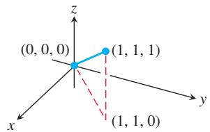
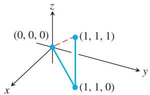
Path 1
Path 2
- The accompanying figure shows three polygonal paths joining the origin to the point (1, 1, 1 . Integrate)
𝑓 ( 𝑥 , 𝑦 , 𝑧 ) = 𝑥 2 + 𝑦 − 𝑧
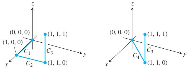
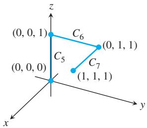
- Integrate
𝑓 ( 𝑥 , 𝑦 , 𝑧 ) = √ 𝑥 2 + 𝑧 2
- Integrate
𝑓 ( 𝑥 , 𝑦 , 𝑧 ) = √ 𝑥 2 + 𝑦 2
Evaluate the integrals in Exercises 5 and 6.
-
Integrate
𝐅 = − ( 𝑦 s i n 𝑧 ) 𝐢 + ( 𝑥 𝑧 ) 𝐣 + ( 𝑥 ) 𝑥 2 + 𝑦 2 + 𝑧 2 = 5 𝑧 = − 1 -
Integrate
𝐅 = 3 𝑥 2 𝑦 𝐢 + ( 𝑥 3 + 1 ) 𝐣 + 9 𝑧 2 𝐤 𝑥 2 + 𝑦 2 + 𝑧 2 = 9 𝑥 = 2
Evaluate the integrals in Exercises 9 and 10.
- ∫ 8 sin 8 cos x y dx y x dy −
C is the square cut from the first quadrant by the lines
∫ 𝐶 𝑦 2 𝑑 𝑥 + 𝑥 2 𝑑 𝑦
C is the circle
Finding and Evaluating Surface Integrals
-
Area of an elliptic region Find the area of the elliptic region cut from the plane
𝑥 + 𝑦 + 𝑧 = . 𝑥 2 + 𝑦 2 = 1 -
Area of a parabolic cap Find the area of the cap cut from the paraboloid
𝑦 2 + 𝑧 2 = 3 𝑥 𝑥 = 1 -
Area of a spherical cap Find the area of the cap cut from the top of the sphere
𝑥 2 + 𝑦 2 + 𝑧 2 = 1 ¯ 𝑧 = √ 2 / 2 -
a. Hemisphere cut by cylinder Find the area of the surface cut from the hemisphere
𝑥 2 + 𝑦 2 + 𝑧 2 = 4 , 𝑧 ≥ 0 , 𝑥 2 + 𝑦 2 = 2 𝑥
b. Find the area of the portion of the cylinder that lies inside the hemisphere. (Hint: Project onto the xz-plane. Or evaluate the integral
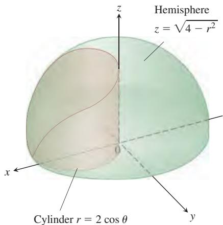
-
Area of a triangle Find the area of the triangle in which the plane
( 𝑥 / 𝑎 ) + ( 𝑦 / 𝑏 ) + ( 𝑧 / 𝑐 ) = 1 ( 𝑎 , 𝑏 , 𝑐 > 0 ) -
Parabolic cylinder cut by planes Integrate
over the surface cut from the parabolic cylinder
-
Circular cylinder cut by planes Integrate
𝑔 ( 𝑥 , 𝑦 , 𝑧 ) = 𝑥 4 𝑦 ( 𝑦 2 + 𝑧 2 ) 𝑦 2 + 𝑧 2 = 2 5 𝑥 = 0 𝑥 = 1 𝑧 = 3 -
Area of Wyoming The state of Wyoming is bounded by the meridians 1
1 1 ∘ 3 ′ 1 0 4 ∘ 3 ′ 4 1 ∘ 4 5 ∘ 𝑅 = 6 3 7 0 k m
Parametrized Surfaces
Find parametrizations for the surfaces in Exercises 19–24. (There are many ways to do these, so your answers may not be the same as those in the back of the text.)
-
Spherical band The portion of the sphere
𝑥 2 + 𝑦 2 + 𝑧 2 = 3 6 𝑧 = − 3 𝑧 = 3 √ 3 -
Parabolic cap The portion of the paraboloid
𝑧 = − ( 𝑥 2 + 𝑦 2 ) / 2 𝑧 = − 2 -
Cone The cone
𝑧 = 1 + √ 𝑥 2 + 𝑦 2 , 𝑧 ≤ 3 -
Plane above square The portion of the plane
4 𝑥 + 2 𝑦 + 4 𝑧 = 0 ≤ 𝑥 ≤ 2 , 0 ≤ 𝑦 ≤ 2 , -
Portion of paraboloid The portion of the paraboloid
𝑦 = 2 ( 𝑥 2 + 𝑧 2 ) , 𝑦 ≤ 2 -
Portion of hemisphere The portion of the hemisphere
𝑥 2 + 𝑦 2 + 𝑧 2 = 1 0 , 𝑦 ≥ 0 , -
Surface area Find the area of the surface
-
Surface integral Integrate
𝑓 ( 𝑥 , 𝑦 , 𝑧 ) = 𝑥 𝑦 − 𝑧 2 -
Area of a helicoid Find the surface area of the helicoid
𝐫 ( 𝑟 , 𝜃 ) = 𝜃 ) 𝐢 + ( 𝑟 s i n 𝜃 ) 𝐣 + 𝜃 𝐤 , 0 ≤ 𝜃 ≤ 2 𝜋 , 0 ≤ 𝑟 ≤ 1 ,
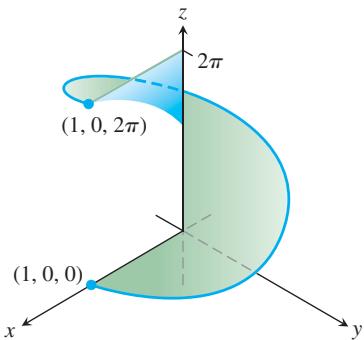
- Surface integral Evaluate the integral
∫ ∫ 𝑆 √ 𝑥 2 + 𝑦 2 + 1 𝑑 𝑦
Conservative Fields
Which of the fields in Exercises 29–32 are conservative, and which are not?
-
𝐅 = 𝑥 𝐢 + 𝑦 𝐣 + 𝑧 𝐤 -
𝐅 = ( 𝑥 𝐢 + 𝑦 𝐣 + 𝑧 𝐤 ) / ( 𝑥 2 + 𝑦 2 + 𝑧 2 ) 3 / 2 -
𝐅 = 𝑥 𝑒 𝑦 𝐢 + 𝑦 𝑒 𝑧 𝐣 + 𝑧 𝑒 𝑥 𝐤 -
𝐅 = ( 𝐢 + 𝑧 𝐣 + 𝑦 𝐤 ) / ( 𝑥 + 𝑦 𝑧 )
Find potential functions for the fields in Exercises 33 and 34.
-
𝐅 = 2 𝐢 + ( 2 𝑦 + 𝑧 ) 𝐣 + ( 𝑦 + 1 ) 𝐤 -
𝐅 = ( 𝑧 c o s 𝑥 𝑧 ) 𝐢 + 𝑒 𝑦 𝐣 + ( 𝑥 c o s 𝑥 𝑧 ) 𝐤
Work and Circulation
In Exercises 35 and 36, find the work done by each field along the paths from (0, 0, 0 to ) (1, 1, 1 in Exercise 1. )
-
F = + + 2xy x i j k2
-
F = + + 2xy x i j k 2
-
Finding work in two ways Find the work done by
over the plane curve r
a. By using the parametrization of the curve to evaluate the work integral.
b. By evaluating a potential function for F.
- Flow along different paths Find the flow of the field
𝐅 = ∇ ( 𝑥 2 𝑧 𝑒 𝑦 )
a. once around the ellipse C in which the plane
b. along the curved boundary of the helicoid in Exercise 27 from (1, 0, 0 to ) (1, 0, 2 .π)
In Exercises 39 and 40, use the curl integral in Stokes’ Theorem to find the circulation of the field F around the curve C in the indicated direction.
- Circulation around an ellipse
𝐅 = 𝑦 2 𝐢 − 𝑦 𝐣 + 3 𝑧 2 𝐤
C: The ellipse in which the plane
- Circulation around a circle
𝐅 = ( 𝑥 2 + 𝑦 ) 𝐢 + ( 𝑥 + 𝑦 ) 𝐣 + ( 4 𝑦 2 − 𝑧 ) 𝐤
C: The circle in which the plane
Masses and Moments
-
Wire with different densities Find the mass of a thin wire lying along the curve
𝐫 ( 𝑡 ) = √ 2 𝑡 𝐢 + √ 2 𝑡 𝐣 + ( 4 − 𝑡 2 ) 𝐤 , 0 ≤ 𝑡 ≤ 1 , ( 𝐚 ) 𝛿 = 3 𝑡 ( 𝐛 ) 𝛿 = 1 -
Wire with variable density Find the center of mass of a thin wire lying along the curve
𝐫 ( 𝑡 ) = 𝑡 𝐢 + 2 𝑡 𝐣 + ( 2 / 3 ) 𝑡 3 / 2 𝐤 , 0 ≤ 𝑡 ≤ 2 , 𝛿 = 3 √ 5 + 𝑡 . -
Wire with variable density Find the center of mass and the moments of inertia about the coordinate axes of a thin wire lying along the curve
if the density at t is
-
Center of mass of an arch A slender metal arch lies along the semicircle
𝑦 = √ 𝑎 2 − 𝑥 2 ( 𝑥 , 𝑦 ) 𝛿 ( 𝑥 , 𝑦 ) = 2 𝑎 − 𝑦 . -
Wire with constant density A wire of constant density
𝛿 = 1 𝐫 ( 𝑡 ) = ( 𝑒 𝑡 c o s 𝑡 ) 𝐢 + ( 𝑒 𝑡 s i n 𝑡 ) 𝐣 + 𝑒 𝑡 𝐤 , 0 ≤ 𝑡 ≤ l n 2 . -
Helical wire with constant density Find the mass and center of mass of a wire of constant density δ that lies along the helix
𝐫 ( 𝑡 ) = ( 2 s i n 𝑡 ) 𝐢 + ( 2 c o s 𝑡 ) 𝐣 + 3 𝑡 𝐤 , 0 ≤ 𝑡 ≤ 2 𝜋 -
Inertia and center of mass of a shell Find
𝐼 𝑧 𝛿 ( 𝑥 , 𝑦 , 𝑧 ) = 𝑧 𝑥 2 + 𝑦 2 + 𝑧 2 = 2 5 𝑧 = 3 -
Moment of inertia of a cube Find the moment of inertia about the z-axis of the surface of the cube cut from the first octant by the planes
𝑥 = 1 , 𝑦 = 1 , a n d 𝑧 = 1 𝛿 = 1
Flux Across a Plane Curve or Surface
Use Green’s Theorem to find the counterclockwise circulation and outward flux for the fields and curves in Exercises 49 and 50.
- Square
𝐅 = ( 2 𝑥 𝑦 + 𝑥 ) 𝐢 + ( 𝑥 𝑦 − 𝑦 ) 𝐣
C: The square bounded by
- Triangle
𝐅 = ( 𝑦 − 6 𝑥 2 ) 𝐢 + ( 𝑥 + 𝑦 2 ) 𝐣
C: The triangle made by the lines
- Zero line integral Show that
for any closed curve C to which Green’s Theorem applies.
- a. Outward flux and area Show that the outward flux of the position vector field
𝐅 = 𝑥 𝐢 + 𝑦 𝐣
b. Let n be the outward unit normal vector to a closed curve to which Green’s Theorem applies. Show that it is not possible for F = + x y i j to be orthogonal to n at every point of C.
In Exercises 53–56, find the outward flux of F across the boundary of D.
- Cube
𝐅 = 2 𝑥 𝑦 𝐢 + 2 𝑦 𝑧 𝐣 + 2 𝑥 𝑧 𝐤
D: The cube cut from the first octant by the planes x = = =1, 1, and 1y z
- Spherical cap
𝐅 = 𝑥 𝑧 𝐢 + 𝑦 𝑧 𝐣 + 𝐤
D: The entire surface of the upper cap cut from the ball
- Spherical cap
𝐅 = − 2 𝑥 𝐢 − 3 𝑦 𝐣 + 𝑧 𝐤
D: The upper region cut from the ball
- Cone and cylinder
𝐅 = ( 6 𝑥 + 𝑦 ) 𝐢 − ( 𝑥 + 𝑧 ) 𝐣 + 4 𝑦 𝑧 𝐤
D: The region in the first octant bounded by the cone
-
Hemisphere, cylinder, and plane Let S be the surface that is bounded on the left by the hemisphere
𝑥 2 + 𝑦 2 + 𝑧 2 = 𝑎 2 , 𝑦 ≤ 0 𝑥 2 + 𝑧 2 = 𝑎 2 , 0 ≤ 𝑦 ≤ 𝑎 𝐅 = y 𝐢 + 𝑧 𝐣 + 𝑥 𝐤 -
Cylinder and planes Find the outward flux of the field
𝐅 = 3 𝑥 𝑧 2 𝐢 + 𝑦 𝐣 − 𝑧 3 𝐤 𝑥 2 + 4 𝑦 2 = 1 6 -
Cylindrical can Use the Divergence Theorem to find the flux of
𝐅 = 𝑥 𝑦 2 𝐢 + 𝑥 2 𝑦 𝐣 + 𝑥 2 + 𝑦 2 = 1 -
Hemisphere Find the flux of
𝐅 = ( 3 𝑧 + 1 ) 𝑥 2 + 𝑦 2 + 𝑧 2 = 𝑎 2 , 𝑧 ≥ 0 , ( 𝐚 )
CHAPTER 15 Additional and Advanced Exercises
Finding Areas with Green’s Theorem
Use the Green’s Theorem area formula in Exercises 15.4 to find the areas of the regions enclosed by the curves in Exercises 1–4.
- The limaçon
𝑥 = 2 c o s 𝑡 − c o s 2 𝑡 , 𝑦 = 2 s i n 𝑡 , 0 ≤ 𝑡 ≤ 2 𝜋
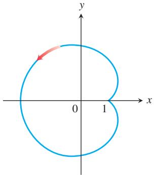
- The deltoid
𝑥 = 2 c o s 𝑡 + c o s 2 𝑡 , 𝑦 = 2 s i n 𝑡 − s i n 2 𝑡 , 0 ≤ 𝑡 ≤ 2 𝜋
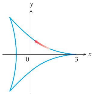
- The eight curve
𝑥 = ( 1 / 2 ) 0 ≤ 𝑡 ≤ 𝜋
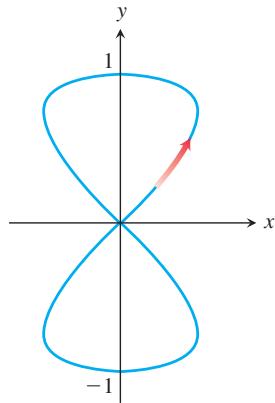
- The teardrop x = − = ≤ ≤ 2 cos sin 2 , sin , 0 2 a t a t y b t t π
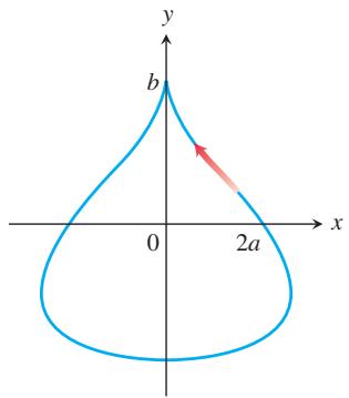
Theory and Applications
- a. Give an example of a vector field
𝐅 ( 𝑥 , 𝑦 , 𝑧 )
b. Give an example of a vector field
c. Give an example of a vector field
-
Find all points
( 𝑎 , 𝑏 , 𝑐 ) 𝑥 2 + 𝑦 2 + 𝑧 2 = 𝑅 2 𝐅 = 𝑦 𝑧 2 𝐢 + 𝑥 𝑧 2 𝐣 + 2 𝑥 ) 𝐅 ( 𝑎 , 𝑏 , 𝑐 ) ≠ 𝟎 . -
Find the mass of a spherical shell of radius R such that at each point
( 𝑥 , 𝑦 , 𝑧 ) 𝛿 ( 𝑥 , 𝑦 , 𝑧 ) ( 𝑎 , 𝑏 , 𝑐 ) -
Find the mass of a helicoid
-
Among all rectangular regions
0 ≤ 𝑥 ≤ 𝑎 , 0 ≤ 𝑦 ≤ 𝑏 , 𝐅 = ( 𝑥 2 + 4 𝑥 𝑦 ) 𝐢 − 6 𝑦 𝐣 -
Find an equation for the plane through the origin such that the circulation of the flow field
𝐅 = 𝑧 𝐢 + 𝑥 𝐣 + 𝛀 . 𝑥 2 + 𝑦 2 + 𝑧 2 = 4 -
A string lies along the circle
𝑥 2 + 𝑦 2 = 4 ( 2 , 0 ) t o ( 0 , 2 ) 𝜌 ( 𝑥 , 𝑦 ) = 𝑥 𝑦
a. Partition the string into a finite number of subarcs to show that the work done by gravity to move the string straight down to the x-axis is given by
where
b. Find the total work done by evaluating the line integral in part (a).
c. Show that the total work done equals the work required to move the string’s center of mass ( x y, straight down to the ) x-axis.
- A thin sheet lies along the portion of the plane
𝑥 + 𝑦 + 𝑧 = 1 𝛿 ( 𝑥 , 𝑦 , 𝑧 ) = 𝑥 𝑦
a. Partition the sheet into a finite number of subpieces to show that the work done by gravity to move the sheet straight down to the xy-plane is given by
where
b. Find the total work done by evaluating the surface integral in part (a).
c. Show that the total work done equals the work required to move the sheet’s center of mass ( x y z , , straight down to the) xy-plane.
- Archimedes’ principle If an object such as a ball is placed in a liquid, it will either sink to the bottom, float, or sink a certain distance and remain suspended in the liquid. Suppose a fluid has constant weight density w and that the fluid’s surface coincides with the plane
𝑧 = 4 𝑥 2 + 𝑦 2 + ( 𝑧 − 2 ) 2 ≤ 1
a. Show that the surface integral giving the magnitude of the total force on the ball due to the fluid’s pressure is
b. Since the ball is not moving, it is being held up by the buoyant force of the liquid. Show that the magnitude of the buoyant force on the sphere is
where n is the outer unit normal at
c. Use the Divergence Theorem to find the magnitude of the buoyant force in part (b).
- Fluid force on a curved surface A cone in the shape of the surface
𝑧 = √ 𝑥 2 + 𝑦 2 , 0 ≤ 𝑧 ≤ 2 , 𝑧 = 1 𝑧 = 2
Evaluate the integral.
- Faraday’s law If
𝐄 ( 𝑡 , 𝑥 , 𝑦 , 𝑧 ) 𝐁 ( 𝑡 , 𝑥 , 𝑦 , 𝑧 ) ( 𝑥 , 𝑦 , 𝑧 ) ∇ × 𝐄 = − 𝜕 𝐁 / 𝜕 𝑡 ∇ × 𝐄 𝜕 𝐁 / 𝜕 𝑡 ( 𝑥 , 𝑦 , 𝑧 )
where C represents a wire loop through which current flows counterclockwise with respect to the surface’s unit normal n, giving rise to the voltage
around C. The surface integral on the right side of the equation is called the magnetic flux, and S is any oriented surface with boundary C.
- Let
be the gravitational force field defined for
- If
𝑓 ( 𝑥 , 𝑦 , 𝑧 ) 𝑔 ( 𝑥 , 𝑦 , 𝑧 )
-
Suppose that
∇ ⋅ 𝐅 1 = ∇ ⋅ 𝐅 2 ∇ × 𝐅 1 = ∇ × 𝐅 2 𝐅 1 ⋅ 𝐧 = 𝐅 2 ⋅ 𝐧 𝐅 1 = 𝐅 2 -
Prove or disprove that if ∇ ⋅ =F 0 and
∇ × 𝐅 = 𝟎 𝐅 = 𝟎 -
Let S be an oriented surface parametrized by
𝐫 ( 𝑢 , 𝑣 ) 𝑑 𝜎 𝜎 = 𝐫 𝑢 𝑑 𝑢 × 𝐫 𝑣 𝑑 \ b o l d s y m b o l 𝜎 = | 𝑑 \ b o l d s y m b o l 𝜎 |
where
- Show that the volume V of a region D in space enclosed by the oriented surface S with outward normal n satisfies the identity
where r is the position vector of the point
CHAPTER 15 Technology Application Projects
Mathematica/Maple Projects
Projects can be found within MyLab Math.
• Work in Conservative and Nonconservative Force Fields Explore integration over vector fields and experiment with conservative and nonconservative force functions along different paths in the field.
• How Can You Visualize Green’s Theorem? Explore integration over vector fields and use parametrizations to compute line integrals. Both forms of Green’s Theorem are explored.
• Visualizing and Interpreting the Divergence Theorem Verify the Divergence Theorem by formulating and evaluating certain divergence and surface integrals.