Chapter 10: Parametric Equations and Polar Coordinates
OVERVIEW In this chapter we study new ways to describe curves in the plane. Instead of considering a curve as the graph of a function or equation, we think of it as the path of a moving particle whose position is changing over time. Then each of the x- and y-coordinates of the particle’s position becomes a function of a third variable t. We can also change the way in which points in the plane themselves are described by using polar coordinates rather than the rectangular or Cartesian system. Both of these new tools are useful for describing motion, like that of planets and satellites, or projectiles moving in the plane or in space.
10.1 Parametrizations of Plane Curves
Parametric Equations
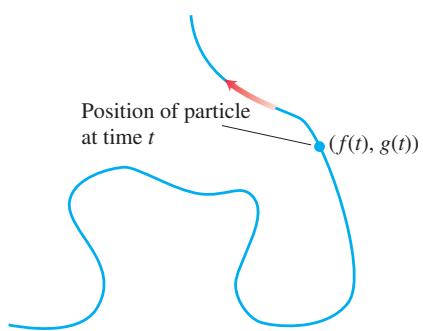
FIGURE 10.1 The curve or path traced by a particle moving in the xy-plane is not always the graph of a function or single equation.
Figure 10.1 shows the path of a moving particle in the xy-plane. Notice that the path fails the vertical line test, so it cannot be described as the graph of a function of the variable x. However, we can describe the path by a pair of equations,
DEFINITION If x and y are given as functions
𝑥 = 𝑓 ( 𝑡 ) , 𝑦 = 𝑔 ( 𝑡 ) over an interval I of t-values, then the set of points
defined by these equations is a parametric curve. The equations are parametric equations for the curve. ( 𝑥 , 𝑦 ) = ( 𝑓 ( 𝑡 ) , 𝑔 ( 𝑡 ) )
The variable t is a parameter for the curve, and its domain I is the parameter interval. If I is a closed interval,
EXAMPLE 1 Sketch the curve defined by the parametric equations
Solution We make a table of values (Table 10.1), plot the points
TABLE 10.1 Values of
| t | x | y |
| 0 | 0 | 0 |
| 1 | 1 | 1 |
| 2 | 0 | 2 |
| 3 | -1 | 3 |
| 4 | 0 | 4 |
| 5 | 1 | 5 |
| 6 | 0 | 6 |
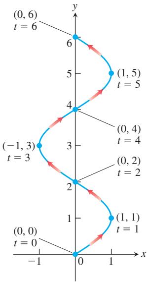
FIGURE 10.2 The curve given by the parametric equations
EXAMPLE 2 Sketch the curve defined by the parametric equations
Solution We make a table of values (Table 10.2), plot the points ( )x y, , and draw a smooth curve through them (Figure 10.3). We think of the curve as the path that a particle moves along the curve in the direction of the arrows. Although the time intervals in the table are equal, the consecutive points plotted along the curve are not at equal arc length distances. The reason for this is that the particle slows down as it gets nearer to the y-axis along the lower branch of the curve as t increases, and then speeds up after reaching the y-axis at 0, 1( ) and moving along the upper branch. Since the interval of values for t is all real numbers, there is no initial point or terminal point for the curve.
TABLE 10.2 Values of
| t | x | y |
| -3 | 9 | -2 |
| -2 | 4 | -1 |
| -1 | 1 | 0 |
| 0 | 0 | 1 |
| 1 | 1 | 2 |
| 2 | 4 | 3 |
| 3 | 9 | 4 |
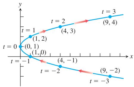
FIGURE 10.3 The curve given by the parametric equations
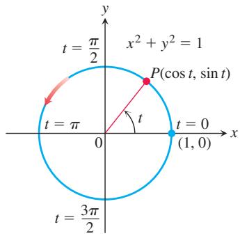
FIGURE 10.4 The equations x = cos t and
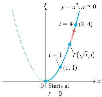
FIGURE 10.5 The equations
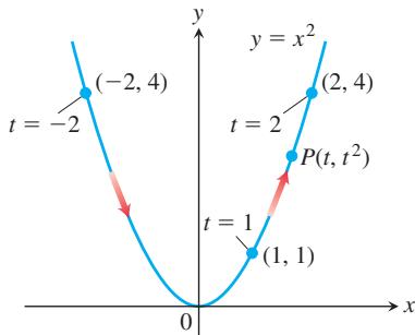
FIGURE 10.6 The path defined by
For this example we can use algebraic manipulation to eliminate the parameter t and obtain an algebraic equation for the curve in terms of x and y alone. We solve
The equation
EXAMPLE 3 Graph the parametric curves
Solution
(a) Since
(b) For
EXAMPLE 4 The position
Identify the path traced by the particle and describe the motion.
Solution We try to identify the path by eliminating t between the equations
Thus, the particle’s position coordinates satisfy the equation
It would be a mistake, however, to conclude that the particle’s path is the entire parabola
The graph of any function
EXAMPLE 5 A parametrization of the graph of the function
When
TABLE 10.3 Values of
| t | 1/t | x | y |
| 0.1 | 10.0 | 10.1 | -9.9 |
| 0.2 | 5.0 | 5.2 | -4.8 |
| 0.4 | 2.5 | 2.9 | -2.1 |
| 1.0 | 1.0 | 2.0 | 0.0 |
| 2.0 | 0.5 | 2.5 | 1.5 |
| 5.0 | 0.2 | 5.2 | 4.8 |
| 10.0 | 0.1 | 10.1 | 9.9 |
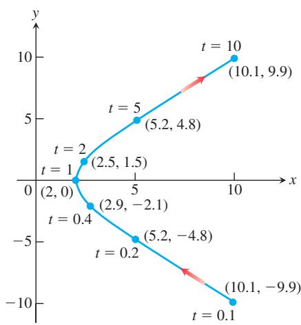
FIGURE 10.7 The curve for
Notice that a parametrization also specifies when a particle moving along the curve is located at a specific point along the curve. In Example 4, the point 2, 4( ) is reached when
EXAMPLE 6 Find a parametrization for the line through the point
Solution A Cartesian equation of the line is
parametrizes the line. This parametrization differs from the one we would obtain by the natural parametrization in Example 5 when
EXAMPLE 7 Sketch and identify the path traced by the point
Solution We make a brief table of values in Table 10.3, plot the points, and draw a smooth curve through them, as we did in Example 1. Next we eliminate the parameter t from the equations. The procedure is more complicated than in Example 2. Taking the difference between x and y as given by the parametric equations, we find that
If we add the two parametric equations, we get
We can then eliminate the parameter t by multiplying these last equations together:
Expanding the expression on the left-hand side, we obtain a standard equation for a hyperbola (Section 10.6):
Thus the coordinates of all the points
Examples 4, 5, and 6 illustrate that a given curve, or portion of it, can be represented by different parametrizations. In the case of Example 7, we can also represent the righthand branch of the hyperbola by the parametrization
which is obtained by solving Equation (1) for
HISTORICAL BIOGRAPHY
Christiaan Huygens (1629–1695)
Huygens was born in the Hague, Netherlands. He studied mathematics at the University of Leiden. Huygens was a follower of Descartes. He published his important geometrical results in Theoremata de quadratura hyperboles, ellipses et circuli and De circuli magnitudine inventa (1654). Later, he considered the subject of probability and published Tractatus de ratiociniis in aleae ludo (1657).
To know more, visit the companion Website.
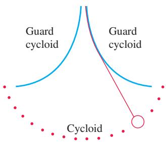
FIGURE 10.8 In Huygens’ pendulum clock, the bob swings in a cycloid, so the frequency is independent of the amplitude.
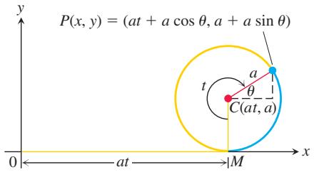
FIGURE 10.9 The position of
This parametrization follows from the trigonometric identity
As t runs between
Cycloids
The problem with a pendulum clock whose bob swings in a circular arc is that the frequency of the swing depends on the amplitude of the swing. The wider the swing, the longer it takes the bob to return to center (its lowest position).
This does not happen if the bob can be made to swing in a curve called a cycloid. In 1673, Christiaan Huygens designed a pendulum clock whose bob would swing in a cycloid, a curve we define in Example 8. He hung the bob from a fine wire constrained by guards that caused it to draw up as it swung away from center (Figure 10.8). We describe the path parametrically in the next example.
EXAMPLE 8 A wheel of radius a rolls along a horizontal straight line. Find parametric equations for the path traced by a point P on the wheel’s circumference. The path is called a cycloid.
Solution We take the line to be the x-axis, mark a point
To express
This makes
The equations we seek are
These are usually written with the a factored out:
Figure 10.10 shows the first arch of the cycloid and part of the next.
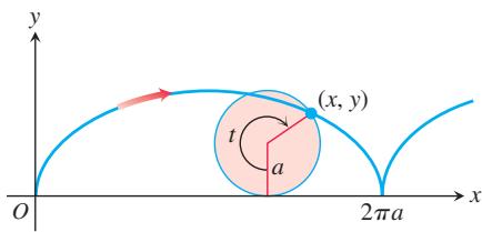
FIGURE 10.10 The cycloid curve x = − = − a t t y a t ( ) ( ) sin , 1 cos , for
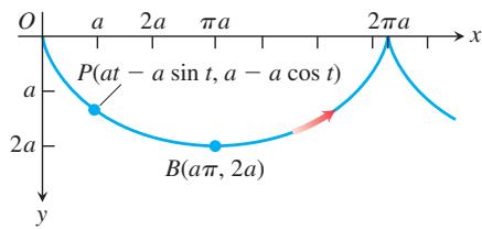
FIGURE 10.11 When Figure 10.10 is turned upside down, the y-axis points downward, indicating the direction of the gravitational force. Equations (2) still describe the curve parametrically.
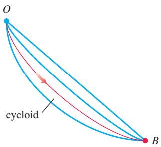
FIGURE 10.12 The cycloid is the unique curve that minimizes the time it takes for a frictionless bead to slide from point O to point B.
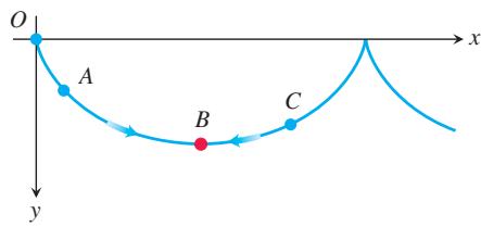
FIGURE 10.13 Beads released simultaneously on the upside-down cycloid at O, A, and C will reach B at the same time.
Brachistochrones and Tautochrones
If we turn Figure 10.10 upside down, Equations (2) still apply and the resulting curve (Figure 10.11) has two interesting physical properties. The first relates to the origin O and the point B at the bottom of the first arch. Among all smooth curves joining these points, the cycloid is the curve along which a frictionless bead, subject only to the force of gravity, will slide from O to B the fastest. This makes the cycloid a brachistochrone (“brah-kisstoe-krone”), or shortest-time curve for these points. The second property is that even if you start the bead partway down the curve toward
Are there any other brachistochrones joining O and B, or is the cycloid the only one? We can formulate this as a mathematical question in the following way. At the start, the kinetic energy of the bead is zero since its velocity (speed) is zero. The work done by gravity in moving the bead from
Thus, the speed of the bead when it reaches
or
The time
What curves
At first sight, we might guess that the straight line joining O and B would give the shortest time, but perhaps not. There might be some advantage in having the bead fall vertically at first to build up its speed faster. With a higher speed, the bead could travel a longer path and still reach B first. Indeed, this is the right idea. The solution, from a branch of mathematics known as the calculus of variations, is that the original cycloid from O to B is the one and only brachistochrone for O and B (Figure 10.12).
In the next section we show how to find the arc length differential ds for a parametrized curve. Once we know how to find
Exercises 10.1
Finding Cartesian from Parametric Equations
Exercises 1–18 give parametric equations and parameter intervals for the motion of a particle in the xy-plane. Identify the particle’s path by finding a Cartesian equation for it. Graph the Cartesian equation. (The graphs will vary with the equation used.) Indicate the portion of the graph traced by the particle and the direction of motion.
-
𝑥 = 3 𝑡 , 𝑦 = 9 𝑡 2 , − ∞ < 𝑡 < ∞ -
𝑥 = − √ 𝑡 , 𝑦 = 𝑡 , 𝑡 ≥ 0 -
𝑥 = 2 𝑡 − 5 , 𝑦 = 4 𝑡 − 7 , − ∞ < 𝑡 < ∞ -
𝑥 = 3 − 3 𝑡 , 𝑦 = 2 𝑡 , 0 ≤ 𝑡 ≤ 1 -
𝑥 = c o s 2 𝑡 , 𝑦 = s i n 2 𝑡 , 0 ≤ 𝑡 ≤ 𝜋 -
𝑥 = c o s ( 𝜋 − 𝑡 ) , 𝑦 = s i n ( 𝜋 − 𝑡 ) , 0 ≤ 𝑡 ≤ 𝜋 -
𝑥 = 4 c o s 𝑡 , 𝑦 = 2 s i n 𝑡 , 0 ≤ 𝑡 ≤ 2 𝜋
E.
-
𝑥 = 4 s i n 𝑡 , 𝑦 = 5 c o s 𝑡 , 0 ≤ 𝑡 ≤ 2 𝜋 -
𝑥 = s i n 𝑡 , 𝑦 = c o s 2 𝑡 , − 𝜋 2 ≤ 𝑡 ≤ 𝜋 2 -
𝑥 = 1 + s i n 𝑡 , 𝑦 = c o s 𝑡 − 2 , 0 ≤ 𝑡 ≤ 𝜋
-
𝑥 = − c o s h 𝑡 , 𝑦 = s i n h 𝑡 , − ∞ < 𝑡 < ∞ -
𝑥 = 2 s i n h 𝑡 , 𝑦 = 2 c o s h 𝑡 , − ∞ < 𝑡 < ∞
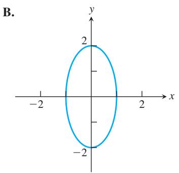
In Exercises 19–24, match the parametric equations with the parametric curves labeled A through F.
-
𝑥 = 1 − s i n 𝑡 , 𝑦 = 1 + c o s 𝑡 -
𝑥 = c o s 𝑡 , 𝑦 = 2 s i n 𝑡 -
𝑥 = 1 4 𝑡 c o s 𝑡 , 𝑦 = 1 4 𝑡 s i n 𝑡 -
𝑥 = √ 𝑡 , 𝑦 = √ 𝑡 c o s 𝑡 -
𝑥 = l n 𝑡 , 𝑦 = 3 𝑒 − 𝑡 / 2 -
𝑥 = c o s 𝑡 , 𝑦 = s i n 3 𝑡
A.
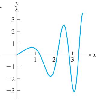
C.
D.
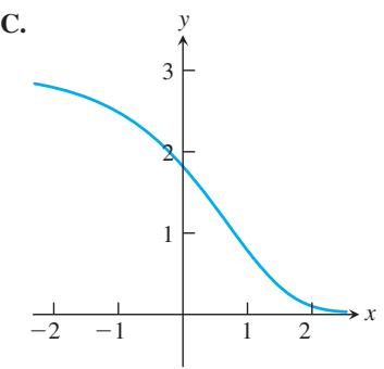
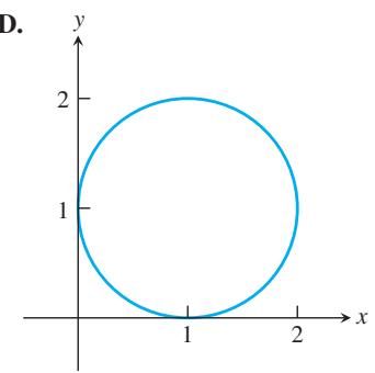
F.
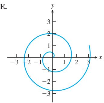
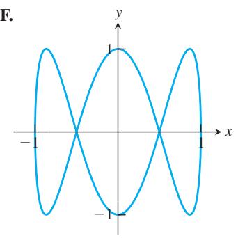
In Exercises 25–28, use the given graphs of
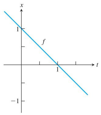
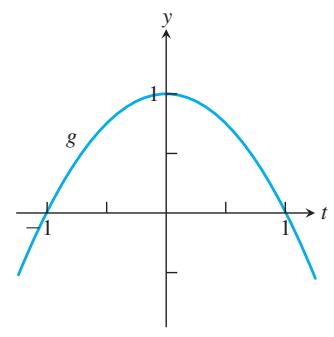
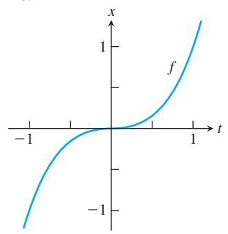
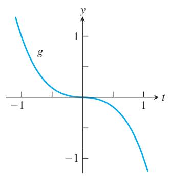
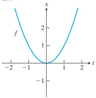
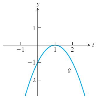
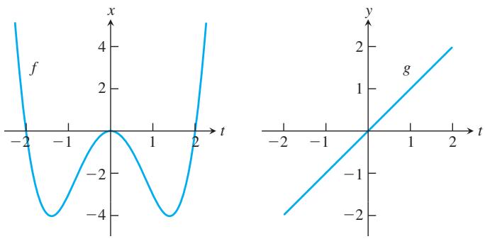
Finding Parametric Equations
- Find parametric equations and a parameter interval for the motion of a particle that starts at
( 𝑎 , 0 ) 𝑥 2 + 𝑦 2 = 𝑎 2
a. once clockwise.
b. once counterclockwise.
c. twice clockwise.
d. twice counterclockwise.
(There are many ways to do these, so your answers may not be the same as the ones at the back of the text.)
- Find parametric equations and a parameter interval for the motion of a particle that starts at
( 𝑎 , 0 ) ( 𝑥 2 / 𝑎 2 ) + ¯ ( 𝑦 2 / 𝑏 2 ) = 1
a. once clockwise.
b. once counterclockwise.
c. twice clockwise.
d. twice counterclockwise.
(As in Exercise 29, there are many correct answers.)
In Exercises 31–36, find a parametrization for the curve.
-
the line segment with endpoints ( ) − − 1, 3 and 4, 1 ( )
-
the line segment with endpoints 1, 3 ( ) − and 3, 2 ( ) −
-
the lower half of the parabola
𝑥 − 1 = 𝑦 2 -
the left half of the parabola
𝑦 = 𝑥 2 + 2 𝑥 -
the ray (half line) with initial point 2, 3( ) that passes through the point ( ) − − 1, 1
-
the ray (half line) with initial point 1, 2 ( ) − that passes through the point ( ) 0, 0
-
Find parametric equations and a parameter interval for the motion of a particle starting at the point ( ) 2, 0 and tracing the top half of the circle
𝑥 2 + 𝑦 2 = 4 -
Find parametric equations and a parameter interval for the motion of a particle that moves along the graph of
𝑦 = 𝑥 2 ( 3 , 9 ) , -
Find parametric equations for the semicircle
using as parameter the slope
- Find parametric equations for the circle
using as parameter the arc length s measured counterclockwise from the point
- Find a parametrization for the line segment joining points ( ) 0, 2 and ( ) 4, 0 using the angle θ in the accompanying figure as the parameter.
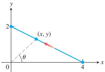
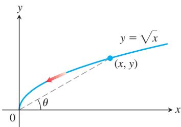
- Find a parametrization for the curve
𝑦 = √ 𝑥
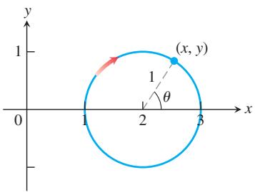
- Find a parametrization for the circle
( 𝑥 − 2 ) 2 + 𝑦 2 = 1
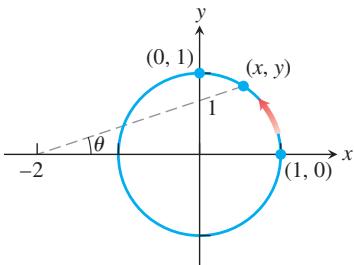
- Find a parametrization for the circle
𝑥 2 + 𝑦 2 = 1
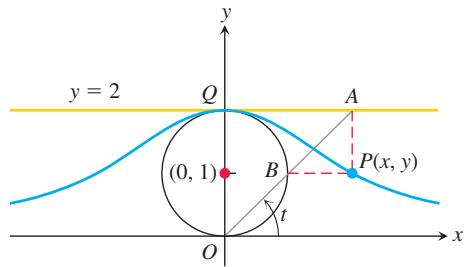
- The witch of Maria Agnesi The bell-shaped witch of Maria Agnesi can be constructed in the following way. Start with a circle of radius 1, centered at the point ( ) 0, 1 , as shown in the accompanying figure. Choose a point A on the line y = 2 and connect it to the origin with a line segment. Call the point where the segment crosses the circle B. Let P be the point where the vertical line through A crosses the horizontal line through B. The witch is the curve traced by P as A moves along the line
𝑦 = 2
a.
c.
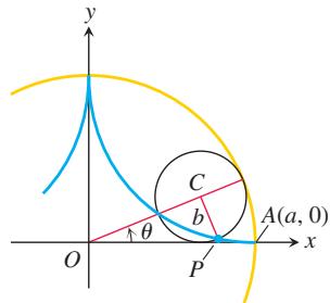
- Hypocycloid When a circle rolls on the inside of a fixed circle, any point P on the circumference of the rolling circle describes a hypocycloid. Let the fixed circle be
𝑥 2 + 𝑦 2 = 𝑎 2 𝑏 , 𝐴 ( 𝑎 , 0 ) i f 𝑏 = 𝑎 / 4
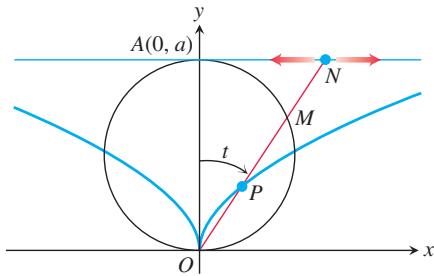
- As the point N moves along the line
𝑦 = 𝑎 𝑂 𝑃 = 𝑀 𝑁
- Trochoids A wheel of radius a rolls along a horizontal straight line without slipping. Find parametric equations for the curve traced out by a point P on a spoke of the wheel b units from its center. As parameter, use the angle θ through which the wheel turns. The curve is called a trochoid, which is a cycloid when
𝑏 = 𝑎 .
Distance Using Parametric Equations
-
Find the point on the parabola
𝑥 = 𝑡 , 𝑦 = 𝑡 2 , − ∞ < 𝑡 < ∞ , -
Find the point on the ellipse x = =2 cos , sin ,t y t
0 ≤ 𝑡 ≤ 2 𝜋
GRAPHER EXPLORATIONST
Using a parametric equation grapher, graph the equations over the given intervals in Exercises 51–58.
- Ellipse x = 4 cos ,t
𝑦 = 2
a.
b.
-
Parabola
𝑥 = 2 𝑡 + 3 , 𝑦 = 𝑡 2 − 1 , − 2 ≤ 𝑡 ≤ 2 -
Cycloid x = −t tsin ,
𝑦 = 1 − c o s 𝑡 ,
a.
b.
c.
- Deltoid
What happens if you replace 2 with −2 in the equations for x and y? Graph the new equations and find out.
- A nice curve
What happens if you replace 3 with −3 in the equations for x and
- a. Epicycloid
b. Hypocycloid
x = + = −8 cos 2 cos 4 , 8 sin 2 sin 4 ,t t y t t
c. Hypotrochoid
x = + = − ≤ ≤cos 5 cos 3 , 6 cos 5 sin 3 , 0 2t t y t t t π
10.2 Calculus with Parametric Curves
In this section we use calculus to study parametric curves. Specifically, we find slopes, lengths, and areas associated with parametrized curves.
Tangent Lines and Areas
A parametrized curve
If
Parametric Formula for dy dx
If all three derivatives exist and
If parametric equations define y as a twice-differentiable function of x, we can apply Equation (1) to the function
Parametric Formula for
If the equations
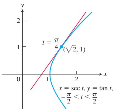
EXAMPLE 1 Find the tangent line to the curve
FIGURE 10.14 The curve in Example 1 is the right-hand branch of the hyperbola
at the point
Solution The slope of the curve at t is
Setting t equal to
The tangent line is
Finding
EXAMPLE 2 Find
- Express
𝑦 ′ = 𝑑 𝑦 /
Solution
-
Find
𝑑 𝑦 ′ / 𝑑 𝑡 . -
Express
𝑦 ′ = 𝑑 𝑦 / 𝑑 𝑥 -
Divide dy dt ′ by dx dt.
- Differentiate
𝑦 ′
- Divide
𝑑 𝑦 ′ / 𝑑 𝑡
EXAMPLE 3 Find the area enclosed by the astroid (Figure 10.15)
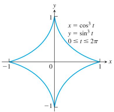
Solution By symmetry, the enclosed area is four times the area beneath the curve in the first quadrant where
FIGURE 10.15 The astroid in Example 3.
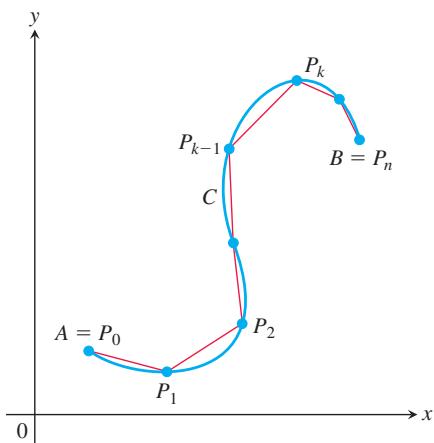
FIGURE 10.16 The length of the smooth curve C from A to B is approximated by the sum of the lengths of the polygonal path (straight-line segments) starting at
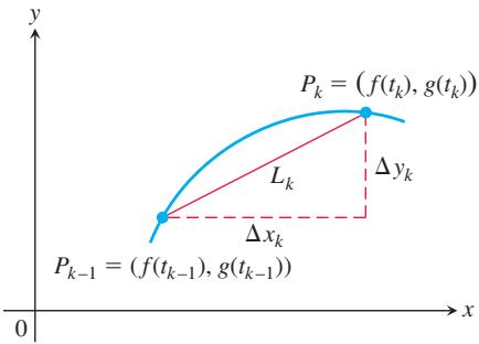
FIGURE 10.17 The arc
Length of a Parametrically Defined Curve
Let C be a curve given parametrically by the equations
We assume the functions
(see Figure 10.17). If
Assuming the path from A to B is traversed exactly once as t increases from
Although this last sum on the right is not exactly a Riemann sum (because
Therefore, it is reasonable to define the length of the curve from A to B to be this integral.
DEFINITION If a curve C is defined parametrically by
and 𝑥 = 𝑓 ( 𝑡 ) 𝑦 = 𝑔 ( 𝑡 ) where 𝑎 ≤ 𝑡 ≤ 𝑏 , and 𝑓 ′ are continuous and not simultaneously zero on [ a, 𝑔 ′ and if C is traversed exactly once as t increases from 𝑏 ] , , then the length of C is the definite integral 𝑡 = 𝑎 t o 𝑡 = 𝑏 . 𝐿 = ∫ 𝑏 𝑎 √ [ 𝑓 ′ ( 𝑡 ) ] 2 + [ 𝑔 ′ ( 𝑡 ) ] 2 𝑑 𝑡 . If
and 𝑥 = 𝑓 ( 𝑡 ) , then using the Leibniz notation we can write the formula for arc length this way: 𝑦 = 𝑔 ( 𝑡 ) 𝐿 = ∫ 𝑏 𝑎 √ ( 𝑑 𝑥 𝑑 𝑡 ) 2 + ( 𝑑 𝑦 𝑑 𝑡 ) 2 𝑑 𝑡 . ( 3 )
A smooth curve C does not come to a stop and reverse its direction of motion over the time interval
If there are two different parametrizations for a curve C whose length we want to find, it does not matter which one we use. However, the parametrization we choose must meet the conditions stated in the definition of the length of C (see Exercise 41 for an example).
EXAMPLE 4 Using the definition, find the length of the circle of radius r defined parametrically by
Solution As t varies from 0 to
We find
and
Therefore, the total arc length is
EXAMPLE 5 Find the length of the astroid (Figure 10.15)
Solution Because of the curve’s symmetry with respect to the coordinate axes, its length is four times the length of the first-quadrant portion. We have
Therefore,
The length of the astroid is four times this:
EXAMPLE 6 Find the perimeter of the ellipse
Solution Parametrically, we represent the ellipse by the equations x
a t sin and
From Equation (3), the perimeter is given by
The integral for P is nonelementary and is known as the complete elliptic integral of the second kind. We can compute its value to within any degree of accuracy using infinite series in the following way. From the binomial expansion for
Then, to each term in this last expression, we apply the integral Formula 157 (at the back of the text) for
Since
Length of a Curve 𝑦 = 𝑓 ( 𝑥 )
We will show that the length formula in Section 6.3 is a special case of Equation (3). Given a continuously differentiable function
which is a special case of what we have considered in this chapter. We have
From Equation (1),
giving
Substitution into Equation (3) gives exactly the arc length formula for the graph of
The Arc Length Differential
As in Section 6.3, we define the arc length function for a parametrically defined curve
Then, by the Fundamental Theorem of Calculus,
The differential of arc length is
Equation (4) is often abbreviated as
Just as in Section 6.3, we can integrate the differential ds between appropriate limits to find the total length of a curve.
Here’s an example where we use the arc length differential to find the centroid of an arc.
EXAMPLE 7 Find the centroid of the first-quadrant arc of the astroid in Example 5.
Solution We take the curve’s density to be
The distribution of mass is symmetric about the line
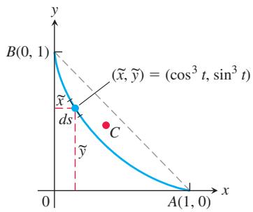
FIGURE 10.18 The centroid C of the astroid arc in Example 7.
The curve’s mass is
The curve’s moment about the x-axis is
It follows that
The centroid is the point ( ) 2 5, 2 5 .
EXAMPLE 8 Find the time
Solution From Equation (3) in Section 10.1, we want to find the time
We need to express
Substituting for ds and y in the integrand, it follows that
This is the amount of time it takes the frictionless bead to slide down the cycloid to B after it is released from rest at O (see Figure 10.13).
Areas of Surfaces of Revolution
In Section 6.4 we found integral formulas for the area of a surface when a curve is revolved about a coordinate axis. Specifically, we found that the surface area is
Area of Surface of Revolution for Parametrized Curves
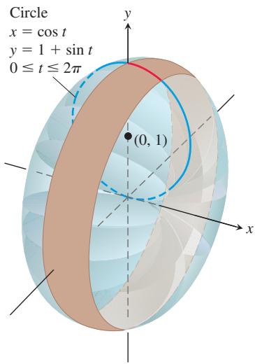
FIGURE 10.19 In Example 9 we calculate the area of the surface of revolution swept out by this parametrized curve.
If a smooth curve
- Revolution about the x-axis
( 𝐲 ≥ 𝟎 )
- Revolution about the y-axis
( 𝑥 𝑥 ≥ 0 0 )
As with length, we can calculate surface area from any convenient parametrization that meets the stated criteria.
EXAMPLE 9 The standard parametrization of the circle of radius 1 centered at the point 0, 1( ) in the xy-plane is
Use this parametrization to find the area of the surface swept out by revolving the circle about the x-axis (Figure 10.19).
Solution We evaluate the formula
EXERCISES 10.2
Tangent Lines to Parametrized Curves
In Exercises 1–14, find an equation for the line tangent to the curve at the point defined by the given value of t. Also, find the value of
-
𝑥 = 2 c o s 𝑡 , 𝑦 = 2 s i n 𝑡 , 𝑡 = 𝜋 / 4 -
𝑥 = s i n 2 𝜋 𝑡 , 𝑦 = c o s 2 𝜋 𝑡 , 𝑡 = − 1 / 6 -
𝑥 = 4 s i n 𝑡 , 𝑦 = 2 c o s 𝑡 , 𝑡 = 𝜋 / 4 -
𝑥 = c o s 𝑡 , 𝑦 = √ 3 c o s 𝑡 , 𝑡 = 2 𝜋 / 3 -
𝑥 = 𝑡 , 𝑦 = √ 𝑡 , 𝑡 = 1 / 4 -
𝑥 = s e c 2 𝑡 − 1 , 𝑦 = t a n 𝑡 , 𝑡 = − 𝜋 / 4 -
𝑥 = s e c 𝑡 , 𝑦 = t a n 𝑡 , 𝑡 = 𝜋 / 6 -
𝑥 = − √ 𝑡 + 1 , 𝑦 = √ 3 𝑡 , 𝑡 = 3 -
𝑥 = 2 𝑡 2 + 3 , 𝑦 = 𝑡 4 , 𝑡 = − 1 -
𝑥 = 1 / 𝑡 , 𝑦 = − 2 + l n 𝑡 , 𝑡 = 1 -
𝑥 = 𝑡 − s i n 𝑡 , 𝑦 = 1 − c o s 𝑡 , 𝑡 = 𝜋 / 3 -
𝑥 = c o s 𝑡 , 𝑦 = 1 + s i n 𝑡 , 𝑡 = 𝜋 / 2 -
𝑥 = 1 𝑡 + 1 , 𝑦 = 𝑡 𝑡 − 1 , 𝑡 = 2 -
𝑥 = 𝑡 + 𝑒 𝑡 , 𝑦 = 1 − 𝑒 𝑡 , 𝑡 = 0
Implicitly Defined Parametrizations
Assuming that the equations in Exercises 15–20 define x and y implicitly as differentiable functions
-
x 2 9, 2 3 4, 2 t y t t 3 2 3 2 + = − = =
-
𝑥 = √ 5 − √ 𝑡 , 𝑦 ( 𝑡 − 1 ) = √ 𝑡 , 𝑡 = 4 -
𝑥 + 2 𝑥 3 / 2 = 𝑡 2 + 𝑡 , 𝑦 √ 𝑡 + 1 + 2 𝑡 √ 𝑦 = 4 , 𝑡 = 0 -
x sin 2 , sin 2 , t x t t t t y t + = − = = π
-
𝑥 = 𝑡 3 + 𝑡 , 𝑦 + 2 𝑡 3 = 2 𝑥 + 𝑡 2 , 𝑡 = 1 -
t x t y te t ln , , 0 t = − = = ( )
Area
- Find the area under one arch of the cycloid
Lengths of Curves
Find the lengths of the curves in Exercises 25–30.
-
𝑥 = c o s 𝑡 , 𝑦 = 𝑡 + s i n 𝑡 , 0 ≤ 𝑡 ≤ 𝜋 -
𝑥 = 𝑡 3 , 𝑦 = 3 𝑡 2 / 2 , 0 ≤ 𝑡 ≤ √ 3 -
𝑥 = 𝑡 2 / 2 , 𝑦 = ( 2 𝑡 + 1 ) 3 / 2 / 3 , 0 ≤ 𝑡 ≤ 4 -
𝑥 = ( 2 𝑡 + 3 ) 3 / 2 / 3 , 𝑦 = 𝑡 + 𝑡 2 / 2 , 0 ≤ 𝑡 ≤ 3 -
x t t t8 cos 8 sin= +
-
x t t tln sec tan sin= + −( )
Surface Area
Find the areas of the surfaces generated by revolving the curves in Exercises 31–34 about the indicated axes.
-
𝑥 = c o s 𝑡 , 𝑦 = 2 + s i n 𝑡 , : : 0 ≤ 𝑡 ≤ 2 -
𝑥 = ( 2 / 3 ) 𝑡 3 / 2 , 𝑦 = 2 √ 𝑡 , 0 ≤ 𝑡 ≤ √ 3 ; -
𝑥 = 𝑡 + √ 2 , 𝑦 = ( 𝑡 2 / 2 ) + √ 2 𝑡 , − √ 2 ≤ 𝑡 ≤ √ 2 ; -
x = + − = ≤ ≤ln sec tan sin , cos , 0 3; -axis( )t t t y t t xπ
-
A cone frustum The line segment joining the points 0, 1( ) and ( ) 2, 2 is revolved about the x-axis to generate a frustum of a cone. Find the surface area of the frustum using the parametrization
𝑥 = 2 𝑡 , 𝑦 = 𝑡 + 1 , 0 ≤ 𝑡 ≤ 1 = 𝜋 ( 𝑟 1 + 𝑟 2 -
A cone The line segment joining the origin to the point
( ℎ , 𝑟 ) 𝑥 = ℎ 𝑡 , 𝑦 = 𝑟 𝑡 , 0 ≤ 𝑡 ≤ 1
Centroids
- Find the coordinates of the centroid of the curve
T 40. Most centroid calculations for curves are done with a calculator or computer that has an integral evaluation program. As a case in point, find, to the nearest hundredth, the coordinates of the centroid of the curve
Theory and Examples
- Length is independent of parametrization To illustrate the fact that the numbers we get for length do not depend on the way we parametrize our curves (except for the mild restrictions preventing doubling back mentioned earlier), calculate the length of the semicircle
𝑦 = √ 1 − 𝑥 2
a.
b. x = = − ≤ ≤ sin , cos , 1 2 1 2. π π t y t t
- a. Show that the Cartesian formula
for the length of the curve
Use this result to find the length of each curve.
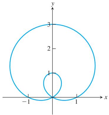
is called a limaçon and is shown in the accompanying figure. Find the points
- The curve with parametric equations
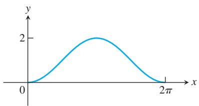
is called a sinusoid and is shown in the accompanying figure. Find the point
a. largest.
b. smallest.
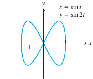
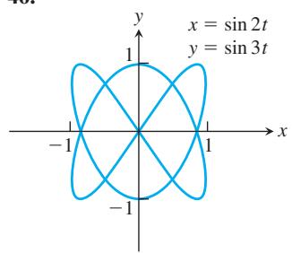
T The curves in Exercises
- Cycloid
a. Find the length of one arch of the cycloid
b. Find the area of the surface generated by revolving one arch of the cycloid in part (a) about the x-axis for
- Volume Find the volume swept out by revolving the region bounded by the x-axis and one arch of the cycloid
about the x-axis.
- Find the volume swept out by revolving the region bounded by the x-axis and the graph of
about the x-axis.
- Find the volume swept out by revolving the region bounded by the y-axis and the graph of
about the y-axis.
COMPUTER EXPLORATIONS
In Exercises 51–54, use a CAS to perform the following steps for the given curve over the closed interval.
a. Plot the curve together with the polygonal path approxima tions for
b. Find the corresponding approximation to the length of the curve by summing the lengths of the line segments.
c. Evaluate the length of the curve using an integral. Compare your approximations for
-
𝑥 = 1 3 𝑡 3 , 𝑦 = 1 2 𝑡 2 , 0 ≤ 𝑡 ≤ 1 -
𝑥 = 2 𝑡 3 − 1 6 𝑡 2 + 2 5 𝑡 + 5 , 𝑦 = 𝑡 2 + 𝑡 − 3 , 0 ≤ 𝑡 ≤ 6 -
x = − = + − ≤ ≤t t y t tcos , 1 sin , Q Q
-
x e t y e t t cos , sin , 0 t t = = ≤ ≤ Q
10.3 Polar Coordinates
In this section we study polar coordinates and their relation to Cartesian coordinates. You will see that polar coordinates are very useful for calculating many multiple integrals studied in Chapter 14. They are also useful in describing the paths of planets and satellites.
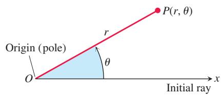
Definition of Polar Coordinates
FIGURE 10.20 To define polar coordinates for the plane, we start with an origin, called the pole, and an initial ray.
To define polar coordinates, we first fix an origin O (called the pole) and an initial ray from O (Figure 10.20). Usually the positive x-axis is chosen as the initial ray. Then each point P can be located by assigning to it a polar coordinate pair
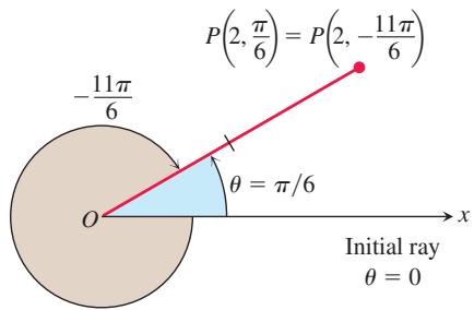
FIGURE 10.21 Polar coordinates are not unique.
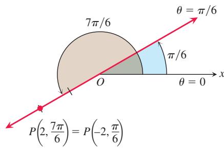
FIGURE 10.22 Polar coordinates can have negative r-values.
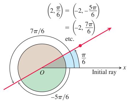
FIGURE 10.23 The point
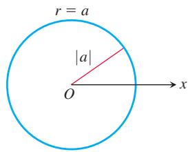
FIGURE 10.24 The polar equation for a circle is r a= .
As in trigonometry, θ is positive when measured counterclockwise and negative when measured clockwise. The angle associated with a given point is not unique. A point in the plane has just one pair of Cartesian coordinates, but it has infinitely many pairs of polar coordinates. For instance, the point 2 units from the origin along the ray
EXAMPLE 1 Find all the polar coordinates of the point
Solution We sketch the initial ray of the coordinate system, draw the ray from the origin that makes an angle of
For
For
The corresponding coordinate pairs of P are
and
When
Polar Equations and Graphs
If we hold r fixed at a constant value
If we hold θ fixed at a constant value
EXAMPLE 2 A circle or line can have more than one polar equation.
(a) r = 1 and
(b)
Equations of the form
(a)
(a)
(b)
(c)
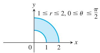
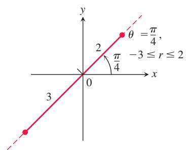
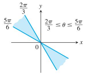
FIGURE 10.25 The graphs of typical inequalities in r and θ (Example 3).
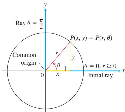
FIGURE 10.26 The usual way to relate polar and Cartesian coordinates.
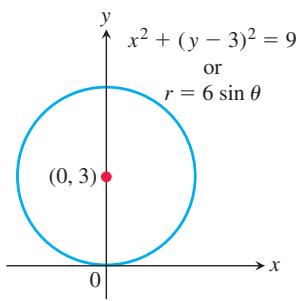
FIGURE 10.27 The circle in Example 5.
EXAMPLE 3 Graph the sets of points whose polar coordinates satisfy the following conditions.
r (no restriction on )
Solution The graphs are shown in Figure 10.25.
Relating Polar and Cartesian Coordinates
When we use both polar and Cartesian coordinates in a plane, we place the two origins together and let the initial polar ray be the positive x-axis. The ray
Equations Relating Polar and Cartesian Coordinates
Polar to Cartesian:
Cartesian to Polar:
The first two of these equations uniquely determine the Cartesian coordinates x and y given the polar coordinates r and θ. On the other hand, if x and y are given and
EXAMPLE 4 Here are some plane curves expressed in terms of both polar coordinate and Cartesian coordinate equations.
| Polar equation | Cartesian equivalent |
Some curves are more simply expressed with polar coordinates; others are not.
EXAMPLE 5 Find a polar equation for the circle
Solution We apply the equations relating polar and Cartesian coordinates:
Expand ( ) y − 3 .2
Cancelation
EXAMPLE 6 Replace the following polar equations by equivalent Cartesian equations and identify their graphs.
(a)
(b)
(c)
Solution We use the substitutions r cos
(a) r cos
rThe Cartesian equation: cos 4θ = −
Substitute.
The graph: Vertical line through x = −4 on the x-axis
(b)
The Cartesian equation:
Substitute.
Complete the square.
Factor.
The graph: Circle, radius
(c)
The Cartesian equation:
Multiply by r.
Substitute.
Solve for y.
The graph: Line, slope m = 2, y-intercept b = −4
EXERCISES 10.3
Polar Coordinates
- Which polar coordinate pairs label the same point?
a.
b.
c. ( ) r, θ
c.
a.
b.
d.
e.
f.
d.
e.
f.
g.
g.
-
Which polar coordinate pairs label the same point?
-
Plot the following points, given in polar coordinates. Then find all the polar coordinates of each point. a.
( 2 , 𝜋 / 2 ) ( − 2 , 𝜋 / 2 ) -
Plot the following points, given in polar coordinates. Then find all the polar coordinates of each point. a. ( ) 3, 4 π b. ( ) −3, 4 π c.
( 3 , − 𝜋 / 4 ) ( − 3 , − 𝜋 / 4 )
Polar to Cartesian Coordinates
-
Find the Cartesian coordinates of the points in Exercise 1.
-
Find the Cartesian coordinates of the following points, given in polar coordinates. a.
( √ 2 , 𝜋 / 4 ) ( 0 , 𝜋 / 2 ) ( − √ 2 , 𝜋 / 4 ) ( − 3 , 5 𝜋 / 6 ) ( 5 , t a n − 1 ( 4 / 3 ) ) ( − 1 , 7 𝜋 ) ( 2 √ 3 , 2 𝜋 / 3 )
Cartesian to Polar Coordinates
-
Find the polar coordinates,
0 ≤ 𝜃 < 2 𝜋 𝑟 ≥ 0 , ( √ 3 , − 1 ) -
Find the polar coordinates,
− 𝜋 ≤ 𝜃 < 𝜋 𝑟 ≥ 0 ( − √ 3 , 1 ) -
Find the polar coordinates,
0 ≤ 𝜃 < 2 𝜋 𝑟 ≤ 0 , ( − 1 , √ 3 ) -
Find the polar coordinates,
− 𝜋 ≤ 𝜃 < 𝜋 𝑟 ≤ 0 ( 0 , − 3 ) ( √ 3 2 , 1 2 )
Graphing Sets of Polar Coordinate Points
Graph the sets of points whose polar coordinates satisfy the equations and inequalities in Exercises 11–26.
-
𝑟 = 2 -
0 ≤ 𝑟 ≤ 2 -
𝑟 ≥ 1 -
1 ≤ 𝑟 ≤ 2 -
0 ≤ 𝜃 ≤ 𝜋 / 6 , 𝑟 ≥ 0 -
𝜃 = 2 𝜋 / 3 , 𝑟 ≤ − 2 -
𝜃 = 𝜋 / 3 , − 1 ≤ 𝑟 ≤ 3 -
𝜃 = 1 1 𝜋 / 4 , 𝑟 ≥ − 1
10.4 Graphing Polar Coordinate Equations
-
𝜃 = 𝜋 / 2 , 𝑟 ≥ 0 -
𝜃 = 𝜋 / 2 , 𝑟 ≤ 0 -
0 ≤ 𝜃 ≤ 𝜋 , 𝑟 = 1 -
0 ≤ 𝜃 ≤ 𝜋 , 𝑟 = − 1 -
𝜋 / 4 ≤ 𝜃 ≤ 3 𝜋 / 4 , 0 ≤ 𝑟 ≤ 1 -
− 𝜋 / 4 ≤ 𝜃 ≤ 𝜋 / 4 , − 1 ≤ 𝑟 ≤ 1 -
− 𝜋 / 2 ≤ 𝜃 ≤ 𝜋 / 2 , 1 ≤ 𝑟 ≤ 2 -
0 ≤ 𝜃 ≤ 𝜋 / 2 , 1 ≤ | 𝑟 | ≤ 2
Polar to Cartesian Equations
Replace the polar equations in Exercises 27–52 with equivalent Cartesian equations. Then describe or identify the graph.
-
𝑟 c o s 𝜃 = 2 -
𝑟 s i n 𝜃 = 0
-
𝑟 = 4 c s c 𝜃 -
𝑟 c o s 𝜃 = 0 -
𝑟 = − 3 s e c 𝜃 -
𝑟 c o s 𝜃 + 𝑟 s i n 𝜃 = 1 -
𝑟 2 = 1 -
𝑟 s i n 𝜃 = 𝑟 c o s 𝜃 -
𝑟 2 = 4 𝑟 s i n 𝜃 -
𝑟 = 5 s i n 𝜃 − 2 c o s 𝜃 -
𝑟 2 s i n 2 𝜃 = 2 -
𝑟 = c o t 𝜃 c s c 𝜃 -
𝑟 = 4 t a n 𝜃 s e c 𝜃 -
𝑟 = c s c 𝜃 𝑒 𝑟 c o s 𝜃 -
𝑟 2 + 2 𝑟 2 c o s 𝜃 s i n 𝜃 = 1 -
𝑟 s i n 𝜃 = l n 𝑟 + l n c o s 𝜃 -
𝑟 2 = − 4 𝑟 c o s 𝜃 -
c o s 2 𝜃 = s i n 2 𝜃 -
𝑟 = 8 s i n 𝜃 -
𝑟 2 = − 6 𝑟 s i n 𝜃 -
𝑟 = 2 c o s 𝜃 + 2 s i n 𝜃 -
𝑟 = 3 c o s 𝜃 -
𝑟 s i n ( 𝜃 + 𝜋 6 ) = 2 -
𝑟 = 2 c o s 𝜃 − s i n 𝜃 -
𝑟 s i n ( 2 𝜋 3 − 𝜃 ) = 5
Cartesian to Polar Equations
Replace the Cartesian equations in Exercises 53–66 with equivalent polar equations.
- x = 7
𝑥 − 𝑦 = 3
-
𝑥 2 9 + 𝑦 2 4 = 1 -
𝑥 𝑦 = 2 -
𝑦 2 = 4 𝑥 -
𝑥 2 + ( 𝑦 − 2 ) 2 = 4 -
𝑥 2 + 𝑥 𝑦 + 𝑦 2 = 1 -
( 𝑥 − 5 ) 2 + 𝑦 2 = 2 5 -
( 𝑥 − 3 ) 2 + ( 𝑦 + 1 ) 2 = 4
- Find all polar coordinates of the origin.
68. Vertical and horizontal lines
a. Show that every vertical line in the xy-plane has a polar equation of the form r a= sec .θ
b. Find the analogous polar equation for horizontal lines in the xy-plane.
It is often helpful to graph an equation expressed in polar coordinates in the Cartesian xy-plane. This section describes some techniques for graphing these equations using symmetries and tangent lines to the graph.
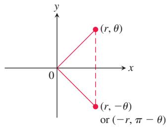
(a) About the x-axis
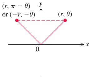
(b) About the y-axis
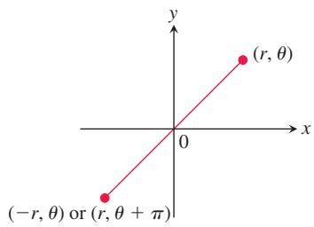
(c) About the origin
FIGURE 10.28 Three tests for symmetry in polar coordinates.
Symmetry
The following list shows how to test for three standard types of symmetries when using polar coordinates. These symmetries are illustrated in Figure 10.28.
Symmetry Tests for Polar Graphs in the Cartesian xy-Plane
-
Symmetry about the x-axis: If the point
( 𝑟 , 𝜃 ) ( 𝑟 , − 𝜃 ) o r ( − 𝑟 , 𝜋 − 𝜃 ) -
Symmetry about the y-axis: If the point
( 𝑟 , 𝜃 ) ( 𝑟 , 𝜋 − 𝜃 ) o r ( − 𝑟 , − 𝜃 ) -
Symmetry about the origin: If the point
( 𝑟 , 𝜃 ) ( − 𝑟 , 𝜃 ) o r ( 𝑟 , 𝜃 + 𝜋 )
Slope
The slope of a polar curve
If
Therefore, we see that
Slope of the Curve
provided
If the curve
That is, the slope at
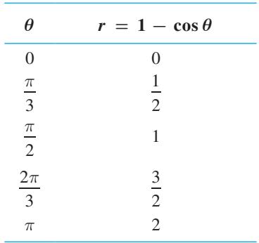
(a)
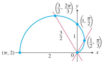
(b)
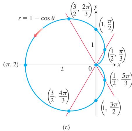
FIGURE 10.29 The steps in graphing the cardioid
EXAMPLE 1 Graph the curve
Solution The curve is symmetric about the x-axis because
As θ increases from 0 to π, cos θ decreases from 1 to −1, and
The curve leaves the origin with slope tan(0) 0 = and returns to the origin with slope
We make a table of values from
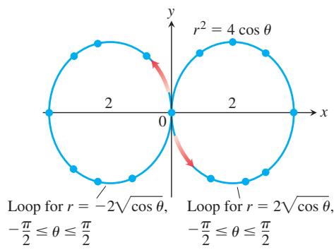
EXAMPLE 2 Graph the curve
Solution The equation
The curve is also symmetric about the origin because
Together, these two symmetries imply symmetry about the y-axis.
The curve passes through the origin when
For each value of θ in the interval between
We make a short table of values, plot the corresponding points, and use information about symmetry and tangent lines to guide us in connecting the points with a smooth curve (Figure 10.30).
| θ | cos θ | r = ±2√cos θ |
| 0 | 1 | ±2 |
| ±π/6 | ≈ ±1.9 | |
| ±π/4 | ≈ ±1.7 | |
| ±π/3 | ≈ ±1.4 | |
| ±π/2 | 0 | 0 |
(a)
(b)
FIGURE 10.30 The graph of
(c)
Converting a Graph from the rT-Plane to the xy-Plane
One way to graph a polar equation
-
First graph the function
𝑟 = 𝑓 ( 𝜃 ) -
Then use that Cartesian graph as a “table” and guide to sketch the polar coordinate graph in the xy-plane.
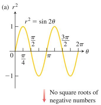
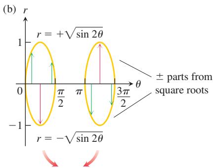
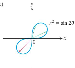
This method is sometimes better than simple point plotting because the first Cartesian graph shows at a glance where r is positive, where negative, and where nonexistent, as well as where r is increasing and where it is decreasing. Here is an example.
EXAMPLE 3 Graph the lemniscate curve
Solution For this example it will be easier to first plot
USING TECHNOLOGY Graphing Polar Curves Parametrically
FIGURE 10.31 To plot
For complicated polar curves, we may need to use a graphing calculator or computer to graph the curve. If the device does not plot polar graphs directly, we can convert
Then we use the device to draw a parametrized curve in the Cartesian xy-plane.
EXERCISES 10.4
Symmetries and Polar Graphs
Identify the symmetries of the curves in Exercises 1–12. Then sketch the curves in the xy-plane.
-
𝑟 = 1 + c o s 𝜃 -
𝑟 = 2 − 2 c o s 𝜃 -
𝑟 = 1 − s i n 𝜃 -
𝑟 = 1 + s i n 𝜃 -
𝑟 = 2 + s i n 𝜃 -
𝑟 = 1 + 2 s i n 𝜃 -
𝑟 = s i n ( 𝜃 / 2 ) -
𝑟 = c o s ( 𝜃 / 2 ) -
r cos 2 = θ
-
𝑟 2 = s i n 𝜃 -
𝑟 2 = − s i n 𝜃 -
𝑟 2 = − c o s 𝜃
Graph the lemniscates in Exercises 13–16. What symmetries do these curves have?
-
𝑟 2 = 4 c o s 2 𝜃 -
𝑟 2 = 4 s i n 2 𝜃 -
𝑟 2 = − s i n 2 𝜃 -
𝑟 2 = − c o s 2 𝜃
Slopes of Polar Curves in the xy-Plane
Find the slopes of the curves in Exercises 17–20 at the given points. Sketch the curves along with their tangent lines at these points.
-
Cardioid
𝑟 = − 1 + c o s 𝜃 ; 𝜃 = ± 𝜋 / 2 -
Cardioid
𝑟 = − 1 + s i n 𝜃 ; 𝜃 = 0 , 𝜋 -
Four-leaved rose
𝑟 = s i n 2 𝜃 ; 𝜃 = ± 𝜋 / 4 , ± 3 𝜋 / 4 -
Four-leaved rose
𝑟 = c o s 2 𝜃 ; 𝜃 = 0 , ± 𝜋 / 2 , 𝜋
Concavity of Polar Curves in the xy-Plane
Equation (1) gives the formula for the derivative
-
r = = sin , 6 , 3 θ θ π π
-
r e = = , 0, θ π θ
-
𝑟 = 𝜃 , 𝜃 = 0 , 𝜋 / 2 -
𝑟 = 1 / 𝜃 , 𝜃 = − 𝜋 , 1
Graphing Limaçons
Graph the limaçons in Exercises 25–28. Limaçon (“lee-ma-sahn”) is Old French for “snail.” You will understand the name when you graph the limaçons in Exercise 25. Equations for limaçons have the form
- Limaçons with an inner loop
Graphing Polar Regions and Curves in the xy-Plane
-
Sketch the region defined by the inequalitie
− 1 ≤ 𝑟 ≤ 2 − 𝜋 / 2 ≤ 𝜃 ≤ 𝜋 / 2 -
Sketch the region defined by the inequalities
0 ≤ 𝑟 ≤ 2 − 𝜋 / 4 ≤ 𝜃 ≤ 𝜋 / 4
In Exercises 31 and 32, sketch the region defined by the inequality.
-
0 ≤ 𝑟 ≤ 2 − 2 -
0 ≤ 𝑟 2 ≤ -
Which of the following has the same graph asT
𝑟 = 1 − c o s 𝜃 ?
a.
Confirm your answer with algebra.
-
Which of the following has the same graph as r = cos 2 ? θT a. r = − + sin 2 2 ( ) θ π b. r = −cos 2 ( ) θ Confirm your answer with algebra.
-
A rose within a rose Graph the equation r = −1 2 sin 3 . θT
-
The nephroid of Freeth Graph the nephroid of Freeth
-
Roses Graph the roses r m = cos θ for m = 1 3, 2, 3, and 7.T
-
Spirals Polar coordinates are just the thing for defining spirals.T Graph the following spirals.
a.
b.
c. A logarithmic spiral:
d. A hyperbolic spiral:
e. An equilateral hyperbola:
(Use different colors for the two branches.)
-
Graph the equationT
𝑟 = s i n ( 8 7 𝜃 ) 0 ≤ 𝜃 ≤ 1 4 𝜋 -
Graph the equationT
for
10.5 Areas and Lengths in Polar Coordinates
This section shows how to calculate areas of plane regions and lengths of curves in polar coordinates.
Area in the Plane
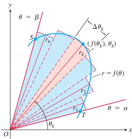
FIGURE 10.32 To derive a formula for the area of region OTS, we approximate the region with fan-shaped circular sectors.
The region OTS in Figure 10.32 is bounded by the rays
The area of region OTS is approximately
If f is continuous, we expect the approximations to improve as the norm of the partition P goes to zero, where the norm of
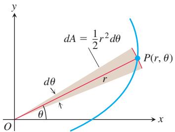
FIGURE 10.33 The area differential dA for the curve
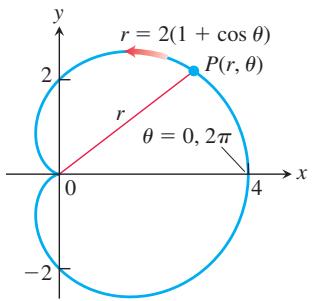
FIGURE 10.34 The cardioid in Example 1.
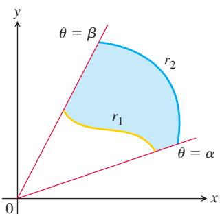
FIGURE 10.35 The area of the shaded region is calculated by subtracting the area of the region between
Area of the Fan-Shaped Region Between the Origin and the Curve
This is the integral of the area differential (Figure 10.33)
In the area formula above, we assumed that
EXAMPLE 1 Find the area of the region in the xy-plane enclosed by the cardioid
Solution We graph the cardioid (Figure 10.34) and determine that the radius
To find the area of a region like the one in Figure 10.35, which lies between two polar curves
Area of the Region
EXAMPLE 2 Find the area of the region that lies inside the circle
Solution We sketch the region to determine its boundaries and find the limits of integration (Figure 10.36). The outer curve is
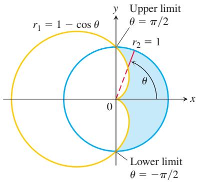
FIGURE 10.36 The region and limits of integration in Example 2.
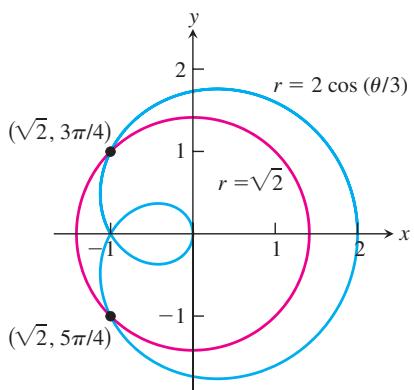
FIGURE 10.37 The curves
The fact that we can represent a point in different ways in polar coordinates requires that we take extra care in deciding when a point lies on the graph of a polar equation and in determining the points at which polar graphs intersect. (We needed intersection points in Example 2.) In Cartesian coordinates, we can always find the points where two curves cross by solving their equations simultaneously. In polar coordinates, the story is different. Simultaneous solution may reveal some intersection points without revealing others, so it is sometimes difficult to find all points of intersection of two polar curves. One way to identify all the points of intersection is to graph the equations.
EXAMPLE 3 Find all of the points where the curve
Solution Note that the function
Solving 2
This gives us one point,
The second intersection point is located at
Length of a Polar Curve
We can obtain a polar coordinate formula for the length of a curve
The parametric length formula, Equation (3) from Section 10.2, then gives the length as
This equation becomes
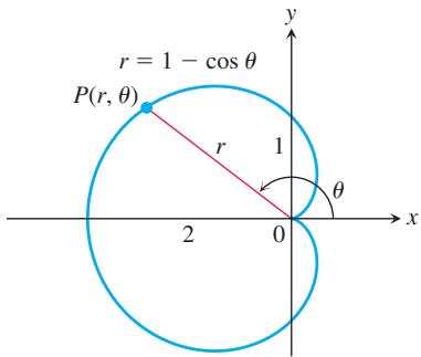
FIGURE 10.38 Calculating the length of a cardioid (Example 4).
when Equations (2) are substituted for x and y (Exercise 29).
Length of a Polar Curve
If
EXAMPLE 4 Find the length of the cardioid
With
Solution We sketch the cardioid to determine the limits of integration (Figure 10.38). The point
we have
and
EXERCISES 10.5
Finding Polar Areas
Find the areas of the regions in Exercises 1–8.
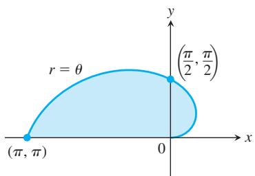
- Bounded by the spiral
𝑟 = 𝜃 0 ≤ 𝜃 ≤ 𝜋
- Bounded by the circle
𝑟 = 2 𝜋 / 4 ≤ 𝜃 ≤ 𝜋 / 2
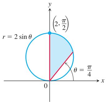
-
Inside the oval limaçon
𝑟 = 4 + 2 -
Inside the cardioid
𝑟 = 𝑎 ( 1 + c o s 𝜃 ) , 𝑎 > 0 -
Inside one leaf of the four-leaved rose
𝑟 = c o s 2 𝜃 -
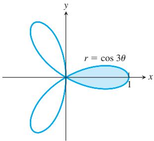
Inside one leaf of the three-leaved rose
𝑟 = c o s 3 𝜃
-
Inside one loop of the lemniscate
𝑟 2 = 4 s i n 2 𝜃 -
Inside the six-leaved rose
𝑟 2 = 2
Find the areas of the regions in Exercises 9–18.
-
Shared by the circles
𝑟 = 2 𝑟 = 2 -
Shared by the circles
𝑟 = 1 𝑟 = 2 -
Shared by the circle
𝑟 = 2 𝑟 = 2 ( 1 − c o s 𝜃 ) -
Shared by the cardioids
𝑟 = 2 ( 1 + c o s 𝜃 ) 𝑟 = 2 ( 1 − c o s 𝜃 ) -
Inside the lemniscate
𝑟 2 = 6 c o s 2 𝜃 𝑟 = √ 3 -
Inside the circle
𝑟 = 3 𝑎 c o s 𝜃 𝑟 = 𝑎 ( 1 + c o s 𝜃 ) , 𝑎 > 0 -
Inside the circle
𝑟 = − 2 𝑟 = 1 -
Inside the circle
𝑟 = 6 𝑟 = 3 -
Inside the circle
𝑟 = 4 c o s 𝜃 𝑟 = s e c 𝜃 -
Inside the circle r = 4 sin θ and below the horizontal line
𝑟 = 3 c s c 𝜃 -
a. Find the area of the shaded region in the accompanying figure.
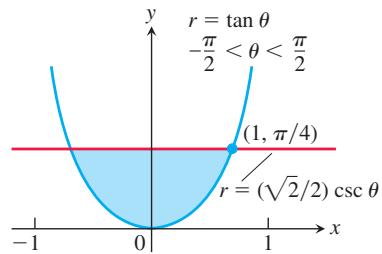
b. It looks as if the graph of r = tan
- The area of the region that lies inside the cardioid curve
𝑟 = c o s 𝜃 + 1 𝑟 = c o s 𝜃
Why not? What is the area? Give reasons for your answers.
Finding Lengths of Polar Curves
Find the lengths of the curves in Exercises 21–28.
-
The spiral
𝑟 = 𝜃 2 , 0 ≤ 𝜃 ≤ √ 5 -
The spiral
𝑟 = 𝑒 𝜃 / √ 2 , 0 ≤ 𝜃 ≤ 𝜋 -
The cardioid
𝑟 = 1 + c o s 𝜃 -
The curve
𝑟 = 𝑎 s i n 2 ( 𝜃 / 2 ) , 0 ≤ 𝜃 ≤ 𝜋 , 𝑎 > 0 -
The parabolic segment
𝑟 = 6 / ( 1 + c o s 𝜃 ) , 0 ≤ 𝜃 ≤ 𝜋 / 2 -
The parabolic segment
𝑟 = 2 / ( 1 − c o s 𝜃 ) , 𝜋 / 2 ≤ 𝜃 ≤ 𝜋 -
The curve
𝑟 = c o s 3 ( 𝜃 / 3 ) , 0 ≤ 𝜃 ≤ 𝜋 / 4 -
The curve
𝑟 = √ 1 + s i n 2 𝜃 , 0 ≤ 𝜃 ≤ 𝜋 √ 2 -
The length of the curve
𝑟 = 𝑓 ( 𝜃 ) , 𝛼 ≤ 𝜃 ≤ 𝛽
(Equations 2 in the text) transform
into
Theory and Examples
- Average value If f is continuous, the average value of the polar coordinate r over the curve
𝑟 = 𝑓 ( 𝜃 ) , 𝛼 ≤ 𝜃 ≤ 𝛽 ,
Use this formula to find the average value of r with respect to R over the following curves
a. The cardioid
b. The circle r a
c. The circle r a = − ≤ ≤ cos , 2 2 θ π θ π
𝑟 = 𝑓 ( 𝜃 ) v s . 𝑟 = 2 𝑓 ( 𝜃 ) 𝑟 = 𝑓 ( 𝜃 ) , 𝛼 ≤ 𝜃 ≤ 𝛽 , 𝑟 = 2 𝑓 ( 𝜃 ) , 𝛼 ≤ 𝜃 ≤ 𝛽 ?
10.6 Conic Sections
In this section we define and review parabolas, ellipses, and hyperbolas geometrically and derive their standard Cartesian equations. These curves are called conic sections or conics because they are formed by cutting a double cone with a plane (Figure 10.39). This
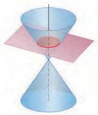
Circle: plane perpendicular to cone axis
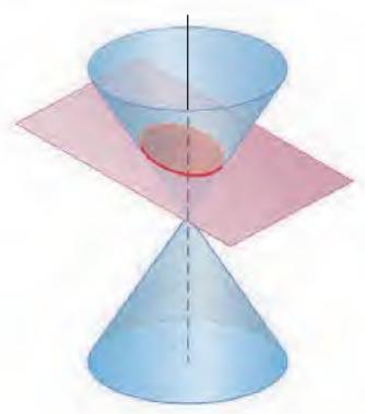
Ellipse: plane oblique to cone axis
(a)
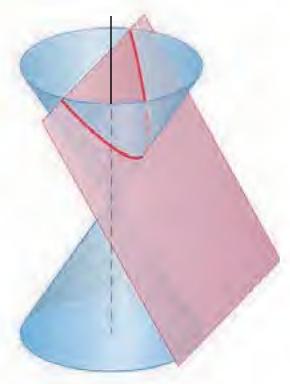
Parabola: plane parallel to side of cone
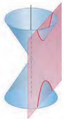
Hyperbola: plane parallel to cone axis
HISTORICAL BIOGRAPHY
Gregory St. Vincent (1584–1667)
Born in Belgium, St. Vincent studied mathematics at Douai. He made important contributions to the development of calculus, and his books were read by the next generation of mathematicians as they connected ideas and refined the concepts of calculus.
To know more, visit the companion Website.
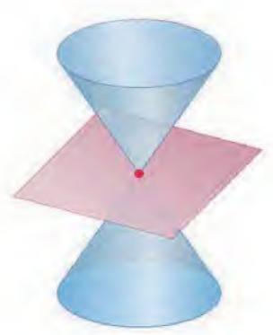
Point: plane through cone vertex only
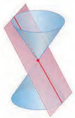
Single line: plane tangent to cone
(b)
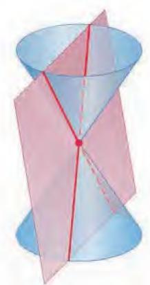
Pair of intersecting lines
FIGURE 10.39 The standard conic sections (a) are the curves in which a plane cuts a double cone. Hyperbolas come in two parts, called branches. The point and lines obtained by passing the plane through the cone’s vertex (b) are degenerate conic sections.
geometric method was the only way that conic sections could be described by Greek mathematicians, since they did not have our tools of Cartesian or polar coordinates. In the next section we express the conics in polar coordinates.
Parabolas
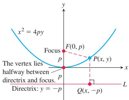
FIGURE 10.40 The standard form of the parabola
DEFINITIONS A set that consists of all the points in a plane equidistant from a given fixed point and a given fixed line in the plane is a parabola. The fixed point is the focus of the parabola. The fixed line is the directrix.
If the focus F lies on the directrix L, the parabola is the line through F perpendicular to L. We consider this to be a degenerate case and assume henceforth that F does not lie on L.
A parabola has its simplest equation when its focus and directrix straddle one of the coordinate axes. For example, suppose that the focus lies at the point
When we equate these expressions, square, and simplify, we get
These equations reveal the parabola’s symmetry about the y-axis. We call the y-axis the axis of the parabola (short for “axis of
The point where a parabola crosses its axis is the vertex. The vertex of the parabola
If the parabola opens downward, with its focus at
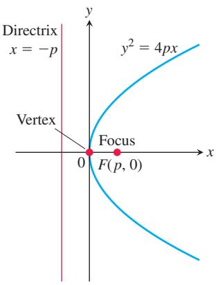
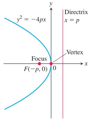
By interchanging the variables x and y, we obtain similar equations for parabolas opening to the right or to the left (Figure 10.41).
(a)
(b)
FIGURE 10.41 (a) The parabola
EXAMPLE 1 Find the focus and directrix of the parabola
Solution We find the value of
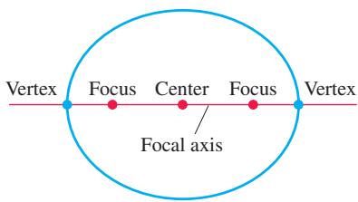
FIGURE 10.42 Points on the focal axis of an ellipse.
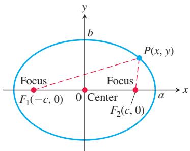
FIGURE 10.43 The ellipse defined by the equation
Then we find the focus and directrix for this value of
Focus:
Directrix:
Ellipses
DEFINITIONS An ellipse is the set of points in a plane whose distances from two fixed points in the plane have a constant sum. The two fixed points are the foci of the ellipse.
The line through the foci of an ellipse is the ellipse’s focal axis. The point on the axis halfway between the foci is the center. The points where the focal axis and ellipse cross are the ellipse’s vertices (Figure 10.42).
If the foci are
To simplify this equation, we move the second radical to the right-hand side, square, isolate the remaining radical, and square again, obtaining
Since
The algebraic steps leading to Equation (2) can be reversed to show that every point P whose coordinates satisfy an equation of this form with
If we let b denote the positive square root of
then
Equation (4) reveals that this ellipse is symmetric with respect to the origin and both coordinate axes. It lies inside the rectangle bounded by the lines
which is zero if
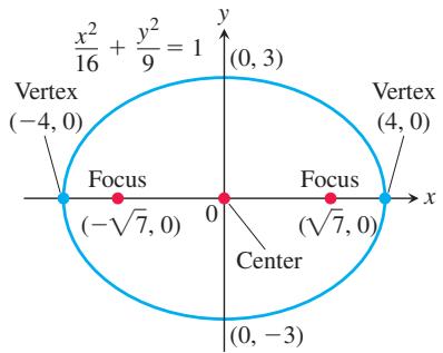
FIGURE 10.44 An ellipse with its major axis horizontal (Example 2).
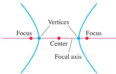
FIGURE 10.45 Points on the focal axis of a hyperbola.
The major axis of the ellipse in Equation (4) is the line segment of length 2a joining the points
is the center-to-focus distance of the ellipse. If
EXAMPLE 2 The ellipse
shown in Figure 10.44 has
Semimajor axis:
Center-to-focus distance:
Foci:
Vertices:
Center: 0, 0 .( )
If we interchange x and y in Equation (5), we have the equation
The major axis of this ellipse is now vertical instead of horizontal, with the foci and vertices on the y-axis. We can determine which way the major axis runs simply by finding the intercepts of the ellipse with the coordinate axes. The longer of the two axes of the ellipse is the major axis.
Standard-Form Equations for Ellipses Centered at the Origin
Foci on the x-axis:
Center-to-focus distance:
Foci: , 0 ( ) ±c
Vertices: , 0 ( ) ±a
Foci on the y-axis:
Center-to-focus distance:
Foci: 0, ( ) ±c
In each case, a is the semimajor axis and b is the semiminor axis.
Hyperbolas
DEFINITIONS A hyperbola is the set of points in a plane whose distances from two fixed points in the plane have a constant difference. The two fixed points are the foci of the hyperbola.
The line through the foci of a hyperbola is the focal axis. The point on the axis halfway between the foci is the hyperbola’s center. The points where the focal axis and hyperbola cross are the vertices (Figure 10.45).
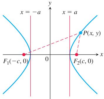
FIGURE 10.46 Hyperbolas have two branches. For points on the right-hand branch of the hyperbola shown here,
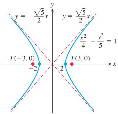
FIGURE 10.47 The hyperbola and its asymptotes in Example 3.
If the foci are
To simplify this equation, we move the second radical to the right-hand side, square, isolate the remaining radical, and square again, obtaining
So far, this looks just like the equation for an ellipse. But now
The algebraic steps leading to Equation (8) can be reversed to show that every point P whose coordinates satisfy an equation of this form with
If we let b denote the positive square root of
then
The differences between Equation (10) and the equation for an ellipse (Equation (4)) are the minus sign and the new relation
Like the ellipse, the hyperbola is symmetric with respect to the origin and coordinate axes. It crosses the x-axis at the points (±a, 0 .) The tangents at these points are vertical because
and this is infinite when
The lines
are the two asymptotes of the hyperbola defined by Equation (10). The fastest way to find the equations of the asymptotes is to replace the 1 in Equation (10) by 0 and solve the new equation for y:
EXAMPLE 3 The equation
is Equation (10) with
Center-to-focus distance:
Foci:
Center: 0, 0 ,( )
Asymptotes:
If we interchange x and y in Equation (11), the foci and vertices of the resulting hyperbola will lie along the y-axis. We still find the asymptotes in the same way as before, but now their equations will be
Standard-Form Equations for Hyperbolas Centered at the Origin
Foci on the x axis :-
: Foci on the y-axis
Center-to-focus distance:
Center-to-focus distance:
Foci:
Foci:
Vertices:
Asymptotes:
Vertices:
Asymptotes:
Notice the difference in the asymptote equations
We shift conics using the principles reviewed in Section 1.2, replacing x by
EXAMPLE 4 Show that the equation
Solution We reduce the equation to standard form by completing the square in x and y as follows:
This is the standard form Equation (10) of a hyperbola with x replaced by
so the asymptotes are the two lines
or
The shifted foci have coordinates
Identifying Graphs
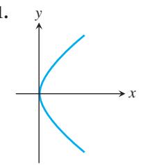
Match the parabolas in Exercises 1–4 with the following equations:
Then find each parabola’s focus and directrix.
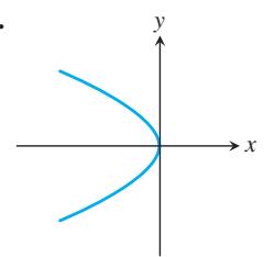
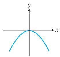
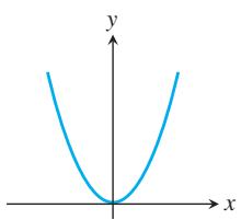
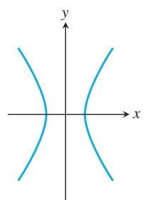
Match each conic section in Exercises 5–8 with one of these equations:
Then find the conic section’s foci and vertices. If the conic section is a hyperbola, find its asymptotes as well.
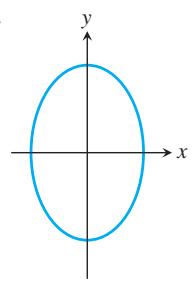
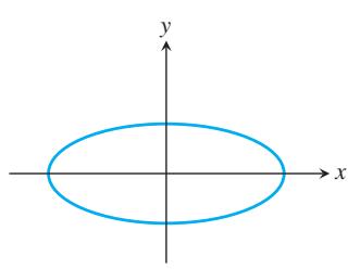
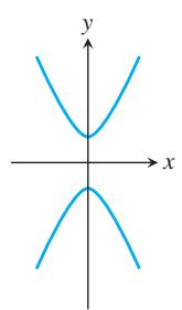
Parabolas
Exercises 9–16 give equations of parabolas. Find each parabola’s focus and directrix. Then sketch the parabola. Include the focus and directrix in your sketch.
-
𝑦 2 = − 2 𝑥 -
𝑦 = 4 𝑥 2
-
𝑥 = − 3 𝑦 2 -
𝑥 = 2 𝑦 2
Ellipses
Exercises 17–24 give equations for ellipses. Put each equation in standard form. Then sketch the ellipse. Include the foci in your sketch.
1 6 𝑥 2 + 2 5 𝑦 2 = 4 0 0
2 𝑥 2 + 𝑦 2 = 2
3 𝑥 2 + 2 𝑦 2 = 6
-
6 𝑥 2 + 9 𝑦 2 = 5 4 -
169 25 4225 x y 2 2 + =
Exercises 25 and 26 give information about the foci and vertices of ellipses centered at the origin of the xy-plane. In each case, find the ellipse’s standard-form equation from the given information.
-
Foci:
( ± √ 2 , 0 ) -
Foci: 0, 4 ( ± ) Vertices: 0, 5 ( ± )
Hyperbolas
Exercises 27–34 give equations for hyperbolas. Put each equation in standard form and find the hyperbola’s asymptotes. Then sketch the hyperbola. Include the asymptotes and foci in your sketch.
-
𝑥 2 − 𝑦 2 = 1 -
9 𝑥 2 − 1 6 𝑦 2 = 1 4 4
- 8x y 2 16 2 2 − =
8 𝑦 2 − 2 𝑥 2 = 1 6
Exercises 35–38 give information about the foci, vertices, and asymptotes of hyperbolas centered at the origin of the xy-plane. In each case, find the hyperbola’s standard-form equation from the information given.
- Foci:
( 0 , ± √ 2 )
Asymptotes: y x = ±
- Foci: 2, 0 (± )
Asymptotes:
- Vertices: (±3, 0)
Asymptotes:
- Vertices: (0, 2± )
Asymptotes:
Shifting Conic Sections
You may wish to review Section 1.2 before solving Exercises 39–56.
- The parabola
𝑦 2 = 8 𝑥 ( 𝑦 + 2 ) 2 = 8 ( 𝑥 − 1 )
a. Find the new parabola’s vertex, focus, and directrix.
b. Plot the new vertex, focus, and directrix, and sketch in the parabola.
- The parabola
𝑥 2 = − 4 𝑦 ( 𝑥 + 1 ) 2 = − 4 ( 𝑦 − 3 )
a. Find the new parabola’s vertex, focus, and directrix.
b. Plot the new vertex, focus, and directrix, and sketch in the parabola.
- The ellipse
( 𝑥 2 / 1 6 ) + ( 𝑦 2 / 9 ) = 1
a. Find the foci, vertices, and center of the new ellipse.
b. Plot the new foci, vertices, and center, and sketch in the new ellipse.
- The ellipse
( 𝑥 2 / 9 ) + ( 𝑦 2 / 2 5 ) = 1
a. Find the foci, vertices, and center of the new ellipse.
b. Plot the new foci, vertices, and center, and sketch in the new ellipse.
- The hyperbola
( 𝑥 2 / 1 6 ) − ( 𝑦 2 / 9 ) = 1
a. Find the center, foci, vertices, and asymptotes of the new hyperbola.
b. Plot the new center, foci, vertices, and asymptotes, and sketch in the hyperbola.
- The hyperbola
( 𝑦 2 / 4 ) − ( 𝑥 2 / 5 ) = 1
a. Find the center, foci, vertices, and asymptotes of the new hyperbola.
b. Plot the new center, foci, vertices, and asymptotes, and sketch in the hyperbola.
Exercises 45–48 give equations for parabolas and tell how many units up or down and to the right or left each parabola is to be shifted. Find an equation for the new parabola, and find the new vertex, focus, and directrix.
-
𝑦 2 = 4 𝑥 -
𝑦 2 = − 1 2 𝑥 -
𝑥 2 = 8 𝑦 , -
𝑥 2 = 6 𝑦
Exercises 49–52 give equations for ellipses and tell how many units up or down and to the right or left each ellipse is to be shifted. Find an equation for the new ellipse, and find the new foci, vertices, and center.
-
𝑥 2 6 + 𝑦 2 9 = 1 -
𝑥 2 2 + 𝑦 2 = 1 -
𝑥 2 3 + 𝑦 2 2 = 1 . -
𝑥 2 1 6 + 𝑦 2 2 5 = 1 ,
Exercises 53–56 give equations for hyperbolas and tell how many units up or down and to the right or left each hyperbola is to be shifted. Find an equation for the new hyperbola, and find the new center, foci, vertices, and asymptotes.
-
𝑥 2 4 − 𝑦 2 5 = 1 , -
𝑥 2 1 6 − 𝑦 2 9 = 1 -
𝑦 2 − 𝑥 2 = 1 , -
𝑦 2 3 − 𝑥 2 = 1 ,
Find the center, foci, vertices, asymptotes, and radius, as appropriate, of the conic sections in Exercises 57–68.
-
𝑥 2 + 4 𝑥 + 𝑦 2 = 1 2 -
2 𝑥 2 + 2 𝑦 2 − 2 8 𝑥 + 1 2 𝑦 + 1 1 4 = 0 -
𝑥 2 + 2 𝑥 + 4 𝑦 − 3 = 0
-
𝑥 2 + 5 𝑦 2 + 4 𝑥 = 1 -
9 𝑥 2 + 6 𝑦 2 + 3 6 𝑦 = 0 -
𝑥 2 + 2 𝑦 2 − 2 𝑥 − 4 𝑦 = − 1 -
4 𝑥 2 + 𝑦 2 + 8 𝑥 − 2 𝑦 = − 1
𝑦 2 − 4 𝑥 2 + 1 6 𝑥 = 2 4
Theory and Examples
- If lines are drawn parallel to the coordinate axes through a point P on the parabola
𝑦 2 = 𝑘 𝑥 , 𝑘 > 0 .
a. If the two smaller regions are revolved about the y-axis, show that they generate solids whose volumes have the ratio 4
.b. What is the ratio of the volumes generated by revolving the regions about the x-axis?
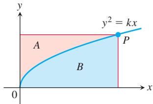
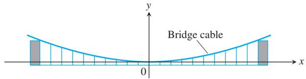
- Suspension bridge cables hang in parabolas The suspension bridge cable shown in the accompanying figure supports a uniform load of w newtons per horizontal meter. It can be shown that if H is the horizontal tension of the cable at the origin, then the curve of the cable satisfies the equation
Show that the cable hangs in a parabola by solving this differential equation subject to the initial condition that
-
The width of a parabola at the focus Show that the number
4 𝑝 𝑥 2 = 4 𝑝 𝑦 ( 𝑝 > 0 ) 𝑦 = 𝑝 -
The asymptotes of
( 𝑥 2 / 𝑎 2 ) − ( 𝑦 2 / 𝑏 2 ) = 1 \ b o l d s y m b o l 𝑦 = ( 𝑏 / 𝑎 ) \ b o l d s y m b o l 𝑥 𝑦 = ( 𝑏 / 𝑎 ) √ 𝑥 2 − 𝑎 2 ( 𝑥 2 / 𝑎 2 ) − ( 𝑦 2 / 𝑏 2 ) = 1
Similar results hold for the remaining portions of the hyperbola and the lines
-
Area Find the dimensions of the rectangle of largest area that can be inscribed in the ellipse
𝑥 2 + 4 𝑦 2 = 4 -
Volume Find the volume of the solid generated by revolving the region enclosed by the ellipse
9 𝑥 2 + 4 𝑦 2 = 3 6 -
Volume The “triangular” region in the first quadrant bounded by the x-axis, the line
𝑥 = 4 ¯ 9 𝑥 2 − 4 𝑦 2 = 3 6 -
Tangents Show that the tangents to the curve
𝑦 2 = 4 𝑝 𝑥 𝑥 = − 𝑝 -
Tangents Find equations for the tangents to the circle
( 𝑥 − 2 ) 2 + ( 𝑦 − 1 ) 2 = 5 -
Volume The region bounded on the left by the y-axis, on the right by the hyperbola
𝑥 2 − 𝑦 2 = 1 𝑦 = ± 3 -
Centroid Find the centroid of the region that is bounded below by the x-axis and above by the ellipse
( 𝑥 2 / 9 ) + ( 𝑦 2 / 1 6 ) = 1
10.7 Conics in Polar Coordinates
-
Surface area The curve
𝑦 = √ 𝑥 2 + 1 , 0 ≤ 𝑥 ≤ √ 2 𝑦 2 − 𝑥 2 = 1 -
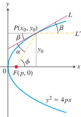
The reflective property of parabolas The accompanying figure shows a typical point
𝑃 ( 𝑥 0 , 𝑦 0 ) 𝑦 2 = 4 𝑝 𝑥 . 𝐹 ( 𝑝 , 0 ) 𝐿 ′ 𝐹 𝑃 𝐿 ′ 𝛽 𝛼 .
a. Show that tan
b. Show that tan
c. Use the identity
to show that tan
Since
Eccentricity
This reflective property of parabolas is used in applications like car headlights, radio telescopes, and satellite TV dishes.
Polar coordinates are especially important in astronomy and astronautical engineering because satellites, moons, planets, and comets all move approximately along ellipses, parabolas, and hyperbolas that can be described with a single relatively simple polar coordinate equation. We develop that equation here after first introducing the idea of a conic section’s eccentricity. The eccentricity reveals the conic section’s type (circle, ellipse, parabola, or hyperbola) and the degree to which it is “squashed” or flattened.
Although the center-to-focus distance c does not appear in the standard Cartesian equation
for an ellipse, we can still determine c from the equation
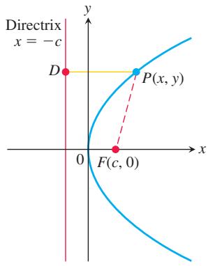
FIGURE 10.48 The distance from the focus F to any point P on a parabola equals the distance from P to the nearest point D on the directrix, so
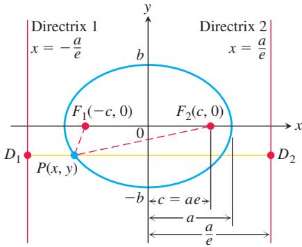
FIGURE 10.49 The foci and directrices of the ellipse
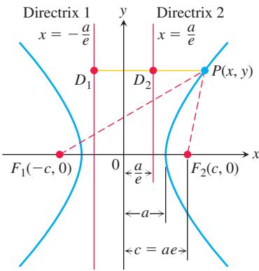
FIGURE 10.50 The foci and directrices of the hyperbola
DEFINITION
The eccentricity of the ellipse
s ( 𝑥 2 / 𝑎 2 ) + ( 𝑦 2 / 𝑏 2 ) = 1 ( 𝑎 > 𝑏 ) 𝐢 𝑒 = 𝑐 𝑎 = √ 𝑎 2 − 𝑏 2 𝑎 . The eccentricity of the hyperbola
is ( 𝑥 2 / 𝑎 2 ) − ( 𝑦 2 / 𝑏 2 ) = 1 𝑒 = 𝑐 𝑎 = √ 𝑎 2 + 𝑏 2 𝑎 . The eccentricity of a parabola is
𝑒 = 1
Whereas a parabola has one focus and one directrix, each ellipse has two foci and two directrices. These are the lines perpendicular to the major axis at distances
for any point P on it, where F is the focus and D is the point nearest P on the directrix. For an ellipse, it can be shown that the equations that replace Equation (1) are
Here, e is the eccentricity, P is any point on the ellipse,
In both Equations (2) the directrix and focus must correspond; that is, if we use the distance from
As with the ellipse, it can be shown that the lines
Here P is any point on the hyperbola,
In both the ellipse and the hyperbola, the eccentricity is the ratio of the distance between the foci to the distance between the vertices (because
In an ellipse, the foci are closer together than the vertices and the ratio is less than 1. In a hyperbola, the foci are farther apart than the vertices and the ratio is greater than 1.
The “focus–directrix” equation
where e is the constant of proportionality. Then the path traced by P is
(a) a parabola if
(b) an ellipse of eccentricity e if
(c) a hyperbola of eccentricity e if
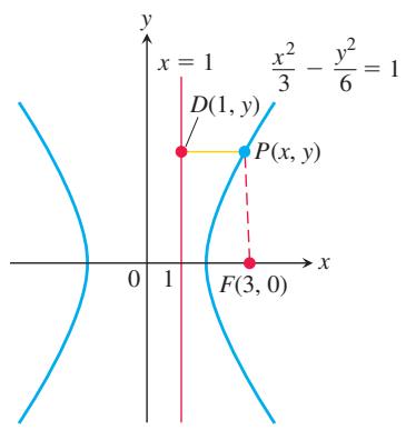
FIGURE 10.51 The hyperbola and directrix in Example 1.
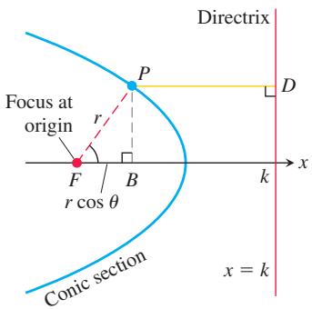
FIGURE 10.52 If a conic section is put in the position with its focus placed at the origin and a directrix perpendicular to the initial ray and right of the origin, we can find its polar equation from the conic’s focus–directrix equation.
As e increases
Given the focus and corresponding directrix of a hyperbola centered at the origin and with foci on the x-axis, we can use the dimensions shown in Figure 10.50 to find e. Knowing
EXAMPLE 1 Find a Cartesian equation for the hyperbola centered at the origin that has a focus at 3, 0( ) and the line
Solution We first use the dimensions shown in Figure 10.50 to find the hyperbola’s eccentricity. The focus is (see Figure 10.51)
Again from Figure 10.50, the directrix is the line
When combined with the equation
Knowing e, we can now derive the equation we want from the equation
Polar Equations
To find a polar equation for an ellipse, parabola, or hyperbola, we place one focus at the origin and the corresponding directrix to the right of the origin along the vertical line
and
The conic’s focus–directrix equation
which can be solved for r to obtain the following expression.
Polar Equation for a Conic with Eccentricity e
where
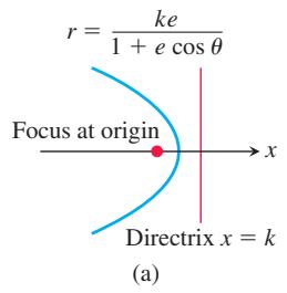
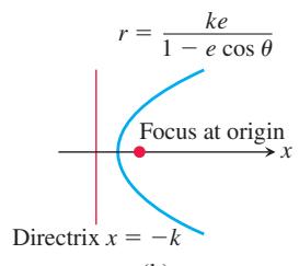
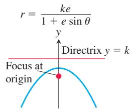
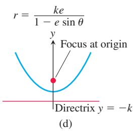
FIGURE 10.53 Equations for conic sections with eccentricity
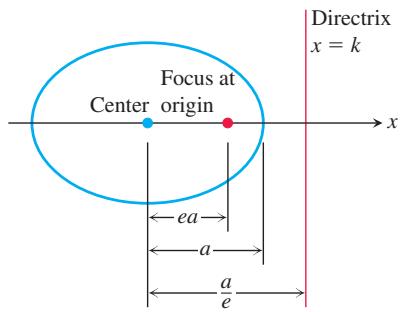
FIGURE 10.54 In an ellipse with semimajor axis a, the focus–directrix distance is
EXAMPLE 2 Here are polar equations for three conics. The eccentricity values identifying the conic are the same for both polar and Cartesian coordinates.
You may see variations of Equation (5), depending on the location of the directrix. If the directrix is the line
The denominator now has a ( ) instead of a − ( ). If the directrix is either of the lines+
EXAMPLE 3 Find an equation for the hyperbola with eccentricity
Solution We use Equation (5) with
EXAMPLE 4 Find the directrix of the parabola
Solution We divide the numerator and denominator by 10 to put the equation in standard polar form:
This is the equation
with
From the ellipse diagram in Figure 10.54, we see that k is related to the eccentricity e and the semimajor axis a by the equation
From this, we find that
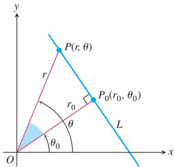
FIGURE 10.55 We can obtain a polar equation for line L by reading the relation
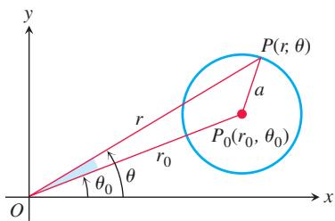
FIGURE 10.56 We can get a polar equation for this circle by applying the Law of Cosines to triangle
Polar Equation for the Ellipse with Eccentricity e and Semimajor Axis a
Notice that when
Lines
Suppose the perpendicular from the origin to line L meets L at the point
The Standard Polar Equation for Lines
If the point
For example, if
Circles
To find a polar equation for the circle of radius a centered at
If the circle passes through the origin, then
If the circle’s center lies on the positive x-axis,
If the center lies on the positive y-axis,
Equations for circles through the origin centered on the negative x- and y-axes can be obtained by replacing r with −r in the above equations.
EXAMPLE 5 Here are several polar equations given by Equations (8) and (9) for circles through the origin and having centers that lie on the x- or y-axis.
| Radius | Center(polar coordinates) | Polar equation |
| 3 | (3, 0) | |
| 2 | (2, | |
| 1/2 | (-1/2, 0) | |
| 1 | (-1, |
EXERCISES 10.7
Ellipses and Eccentricity
In Exercises 1–8, find the eccentricity of the ellipse. Then find and graph the ellipse’s foci and directrices.
-
1 6 𝑥 2 + 2 5 𝑦 2 = 4 0 0 -
7x y + = 16 112 2 2
-
2 𝑥 2 + 𝑦 2 = 2 -
2 4 x y 2 2 + =
-
3 𝑥 2 + 2 𝑦 2 = 6 -
9 𝑥 2 + 1 0 𝑦 2 = 9 0 -
6 𝑥 2 + 9 𝑦 2 = 5 4 -
169 25 4225x y2 2 + =
Exercises 9–12 give the foci or vertices and the eccentricities of ellipses centered at the origin of the xy-plane. In each case, find the ellipse’s standard-form equation in Cartesian coordinates.
-
Foci: ( ) 0, 3 ± Eccentricity: 0.5
-
Foci: ( ) ±8, 0 Eccentricity: 0.2
Exercises 13–16 give foci and corresponding directrices of ellipses centered at the origin of the xy-plane. In each case, use the dimensions in Figure 10.49 to find the eccentricity of the ellipse. Then find the ellipse’s standard-form equation in Cartesian coordinates.
-
Vertices: ( ) 0, 70± Eccentricity: 0.1
-
Focus:
( √ 5 , 0 ) 𝑥 = 9 √ 5 -
Focus: ( ) 4, 0
-
Focus: ( ) −4, 0 Directrix:
𝑥 = − 1 6 -
Focus:
( − √ 2 , 0 ) 𝑥 = − 2 √ 2
Hyperbolas and Eccentricity
In Exercises 17–24, find the eccentricity of the hyperbola. Then find and graph the hyperbola’s foci and directrices. 17.
8 𝑥 2 − 2 𝑦 2 = 1 6
𝑦 2 − 3 𝑥 2 = 3 6 4 𝑥 2 − 3 6 𝑦 2 = 2 3 0 4
Exercises 25–28 give the eccentricities and the vertices or foci of hyperbolas centered at the origin of the xy-plane. In each case, find the hyperbola’s standard-form equation in Cartesian coordinates.
-
Eccentricity: 3 Vertices: ( ) 0, 1 ±
-
Eccentricity: 2 Vertices: ( ) ±2, 0
-
Eccentricity: 3 Foci: ( ) ±3, 0
-
Eccentricity: 1.25 Foci: ( ) 0, 5 ±
Eccentricities and Directrices
Exercises 29–36 give the eccentricities of conic sections with one focus at the origin along with the directrix corresponding to that focus. Find a polar equation for each conic section.
-
𝑒 = 1 , 𝑥 = 2 -
𝑒 = 1 , 𝑦 = 2 -
𝑒 = 5 , 𝑦 = − 6 -
𝑒 = 2 , 𝑥 = 4 -
𝑒 = 1 / 2 , 𝑥 = 1 -
𝑒 = 1 / 4 , 𝑥 = − 2 -
𝑒 = 1 / 5 , 𝑦 = − 1 0 -
𝑒 = 1 / 3 , 𝑦 = 6
Parabolas and Ellipses
Sketch the parabolas and ellipses in Exercises 37–44. Include the directrix that corresponds to the focus at the origin. Label the vertices with appropriate polar coordinates. Label the centers of the ellipses as well.
-
𝑟 = 1 1 + c o s 𝜃 -
𝑟 = 6 2 + c o s 𝜃 -
𝑟 = 2 5 1 0 − 5 c o s 𝜃 -
𝑟 = 4 2 − 2 c o s 𝜃 -
𝑟 = 4 0 0 1 6 + 8 s i n 𝜃 -
𝑟 = 1 2 3 + 3 s i n 𝜃 -
𝑟 = 8 2 − 2 s i n 𝜃 -
𝑟 = 4 2 − s i n 𝜃
Lines
Sketch the lines in Exercises 45–48 and find Cartesian equations for them.
-
𝑟 c o s ( 𝜃 − 𝜋 4 ) = √ 2 -
𝑟 c o s ( 𝜃 + 3 𝜋 4 ) = 1 -
𝑟 c o s ( 𝜃 − 2 𝜋 3 ) = 3 -
𝑟 c o s ( 𝜃 + 𝜋 3 ) = 2
Find a polar equation in the form r cos
-
√ 2 𝑥 + √ 2 𝑦 = 6 -
√ 3 𝑥 − 𝑦 = 1 -
𝑦 = − 5 -
𝑥 = − 4
Circles
Sketch the circles in Exercises 53–56. Give polar coordinates for their centers and identify their radii
-
𝑟 = 4 c o s 𝜃 -
𝑟 = 6 s i n 𝜃 -
𝑟 = − 2 c o s 𝜃 -
𝑟 = − 8 s i n 𝜃
Find polar equations for the circles in Exercises 57–64. Sketch each circle in the coordinate plane and label it with both its Cartesian and polar equations.
-
( 𝑥 − 6 ) 2 + 𝑦 2 = 3 6 -
( 𝑥 + 2 ) 2 + 𝑦 2 = 4 -
𝑥 2 + ( 𝑦 − 5 ) 2 = 2 5 -
𝑥 2 + ( 𝑦 + 7 ) 2 = 4 9 -
𝑥 2 + 2 𝑥 + 𝑦 2 = 0 -
𝑥 2 − 1 6 𝑥 + 𝑦 2 = 0 -
𝑥 2 + 𝑦 2 + 𝑦 = 0 -
𝑥 2 + 𝑦 2 − 4 3 𝑦 = 0
Examples of Polar Equations
Graph the lines and conic sections in Exercises 65–74.T
-
𝑟 = 3 s e c ( 𝜃 − 𝜋 / 3 ) -
𝑟 = 4 s e c ( 𝜃 + 𝜋 / 6 ) -
𝑟 = 4 s i n 𝜃 -
𝑟 = − 2 c o s 𝜃 -
𝑟 = 8 / ( 4 + c o s 𝜃 ) -
𝑟 = 8 / ( 4 + s i n 𝜃 )
CHAPTER 10 Questions to Guide Your Review
-
What is a parametrization of a curve in the xy-plane? Does a function
𝑦 = 𝑓 ( 𝑥 ) -
Give some typical parametrizations for lines, circles, parabolas, ellipses, and hyperbolas. How might the parametrized curve differ from the graph of its Cartesian equation?
-
What is a cycloid? What are typical parametric equations for cycloids? What physical properties account for the importance of cycloids?
-
What is the formula for the slope
𝑑 𝑦 / 𝑑 𝑥 𝑥 = 𝑓 ( 𝑡 ) , 𝑦 = 𝑔 ( 𝑡 ) ? 𝑑 2 𝑦 / 𝑑 𝑥 2 -
How can you sometimes find the area bounded by a parametrized curve and one of the coordinate axes?
-
𝑟 = 1 / ( 1 − s i n 𝜃 )
𝑟 = 1 / ( 1 + 2 s i n 𝜃 )
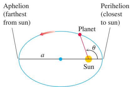
- Perihelion and aphelion A planet travels about its sun in an ellipse whose semimajor axis has length a. (See accompanying figure.)
a. Show that
b. Use the data in the table in Exercise 76 to find how close each planet in our solar system comes to the sun and how far away each planet gets from the sun.
- Planetary orbits Use the data in the table below and Equation (6) to find polar equations for the orbits of the planets.
| Planet | Semimajor axis (astronomical units) | Eccentricity |
| Mercury | 0.3871 | 0.2056 |
| Venus | 0.7233 | 0.0068 |
| Earth | 1.000 | 0.0167 |
| Mars | 1.524 | 0.0934 |
| Jupiter | 5.203 | 0.0484 |
| Saturn | 9.539 | 0.0543 |
| Uranus | 19.18 | 0.0460 |
| Neptune | 30.06 | 0.0082 |
-
How do you find the length of a smooth parametrized curve
𝑥 = 𝑓 ( 𝑡 ) , 𝑦 = 𝑔 ( 𝑡 ) , 𝑎 ≤ 𝑡 ≤ 𝑏 ? -
What is the arc length function for a smooth parametrized curve? What is its arc length differential?
-
Under what conditions can you find the area of the surface generated by revolving a curve
𝑥 = 𝑓 ( 𝑡 ) , 𝑦 = 𝑔 ( 𝑡 ) , 𝑎 ≤ 𝑡 ≤ 𝑏 . -
What are polar coordinates? What equations relate polar coordinates to Cartesian coordinates? Why might you want to change from one coordinate system to the other?
-
What consequence does the lack of uniqueness of polar coordinates have for graphing? Give an example.
-
How do you graph equations in polar coordinates? Include in your discussion symmetry, slope, behavior at the origin, and the use of Cartesian graphs. Give examples.
-
How do you find the area of a region
0 ≤ 𝑟 1 ( 𝜃 ) ≤ 𝑟 ≤ 𝑟 2 ( 𝜃 ) 𝛼 ≤ 𝜃 ≤ 𝛽 , -
Under what conditions can you find the length of a curve
𝑟 = 𝑓 ( 𝜃 ) , 𝛼 ≤ 𝜃 ≤ 𝛽 , -
What is a parabola? What are the Cartesian equations for parabolas whose vertices lie at the origin and whose foci lie on the coordinate axes? How can you find the focus and directrix of such a parabola from its equation?
-
What is an ellipse? What are the Cartesian equations for ellipses centered at the origin with foci on one of the coordinate axes?
How can you find the foci, vertices, and directrices of such an ellipse from its equation?
-
What is a hyperbola? What are the Cartesian equations for hyperbolas centered at the origin with foci on one of the coordinate axes? How can you find the foci, vertices, and directrices of such an ellipse from its equation?
-
What is the eccentricity of a conic section? How can you classify conic sections by eccentricity? How does eccentricity change the shape of ellipses and hyperbolas?
-
Explain the equation
𝑃 𝐹 = 𝑒 ⋅ 𝑃 𝐷 . -
What are the standard equations for lines and conic sections in polar coordinates? Give examples.
CHAPTER 10 Practice Exercises
Identifying Parametric Equations in the Plane
Exercises 1–6 give parametric equations and parameter intervals for the motion of a particle in the xy-plane. Identify the particle’s path by finding a Cartesian equation for it. Graph the Cartesian equation and indicate the direction of motion and the portion traced by the particle.
-
𝑥 = 𝑡 / 2 , 𝑦 = 𝑡 + 1 , − ∞ < 𝑡 < ∞ -
𝑥 = √ 𝑡 , 𝑦 = 1 − √ 𝑡 , 𝑡 ≥ 0 -
𝑥 = ( 1 / 2 ) t a n 𝑡 , 𝑦 = ( 1 / 2 ) s e c 𝑡 , − 𝜋 / 2 < 𝑡 < 𝜋 / 2 -
𝑥 = − 2 c o s 𝑡 , 𝑦 = 2 s i n 𝑡 , 0 ≤ 𝑡 ≤ 𝜋 -
𝑥 = − c o s 𝑡 , 𝑦 = c o s 2 𝑡 , 0 ≤ 𝑡 ≤ 𝜋 -
𝑥 = 4 c o s 𝑡 , 𝑦 = 9 s i n 𝑡 , 0 ≤ 𝑡 ≤ 2 𝜋
Finding Parametric Equations and Tangent Lines
-
Find parametric equations and a parameter interval for the motion of a particle in the xy-plane that traces the ellipse
1 6 𝑥 2 + 9 𝑦 2 = 1 4 4 -
Find parametric equations and a parameter interval for the motion of a particle that starts at the point ( ) −2, 0 in the xy-plane and traces the circle
𝑥 2 + 𝑦 2 = 4
In Exercises 9 and 10, find an equation for the line in the xy-plane that is tangent to the curve at the point corresponding to the given value of t. Also, find the value of
-
𝑥 = ( 1 / 2 ) t a n 𝑡 , 𝑦 = ( 1 / 2 ) s e c 𝑡 , 𝑡 = 𝜋 / 3 -
𝑥 = 1 + 1 / 𝑡 2 , 𝑦 = 1 − 3 / 𝑡 , 𝑡 = 2 -
Eliminate the parameter to express the curve in the form
𝑦 = 𝑓 ( 𝑥 ) -
Find parametric equations for the given curve.
b. x = = cos , tan t y t
a. Line through ( ) 1, 2 with slope 3 −
Lengths of Curves
Find the lengths of the curves in Exercises 13–19.
-
𝑦 = 𝑥 1 / 2 − ( 1 / 3 ) 𝑥 3 / 2 , 1 ≤ 𝑥 ≤ 4 -
𝑥 = 𝑦 2 / 3 , 1 ≤ 𝑦 ≤ 8 -
𝑦 = ( 5 / 1 2 ) 𝑥 6 / 5 − ( 5 / 8 ) 𝑥 4 / 5 , 1 ≤ 𝑥 ≤ 3 2 -
𝑥 = ( 𝑦 3 / 1 2 ) + ( 1 / 𝑦 ) , 1 ≤ 𝑦 ≤ 2 -
x = − = − ≤ ≤ 5 cos cos 5 , 5 sin sin 5 , 0 2 t t y t t t π
-
𝑥 = 𝑡 3 − 6 𝑡 2 , 𝑦 = 𝑡 3 + 6 𝑡 2 , 0 ≤ 𝑡 ≤ 1 -
𝑥 = 3 c o s 𝜃 , 𝑦 = 3 s i n 𝜃 , 0 ≤ 𝜃 ≤ 3 𝜋 2 -
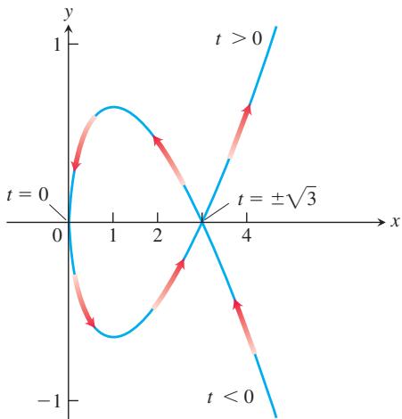
Find the length of the enclosed loop
𝑥 = 𝑡 2 , 𝑦 = ( 𝑡 3 / 3 ) − 𝑡 𝑡 = − √ 3 𝑡 = √ 3
Surface Areas
Find the areas of the surfaces generated by revolving the curves in Exercises 21 and 22 about the indicated axes.
-
𝑥 = 𝑡 2 / 2 , 𝑦 = 2 𝑡 , 0 ≤ 𝑡 ≤ √ 5 , -
𝑥 = 𝑡 2 + 1 / ( 2 𝑡 ) , 𝑦 = 4 √ 𝑡 , 1 / √ 2 ≤ 𝑡 ≤ 1 ,
Polar to Cartesian Equations
Sketch the lines in Exercises 23–28. Also, find a Cartesian equation for each line.
-
𝑟 c o s ( 𝜃 + 𝜋 3 ) = 2 √ 3 -
𝑟 c o s ( 𝜃 − 3 𝜋 4 ) = √ 2 2 -
𝑟 = 2 s e c 𝜃
𝑟 = ( 3 √ 3 ) c s c 𝜃
Find Cartesian equations for the circles in Exercises 29–32. Sketch each circle in the coordinate plane and label it with both its Cartesian and polar equations.
-
𝑟 = 3 √ 3 s i n 𝜃 -
𝑟 = 2 √ 2 c o s 𝜃
Cartesian to Polar Equations
Find polar equations for the circles in Exercises 33–36. Sketch each circle in the coordinate plane and label it with both its Cartesian and polar equations.
Graphs in Polar Coordinates
Sketch the regions defined by the polar coordinate inequalities in Exercises 37 and 38.
− 4 s i n 𝜃 ≤ 𝑟 ≤ 0
Match each graph in Exercises 39–46 with the appropriate equation (a)–(l). There are more equations than graphs, so some equations will not be matched.
-
Four-leaved rose
-
Spiral
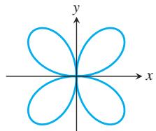
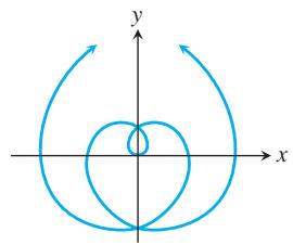
-
Limaçon
-
Lemniscate
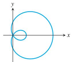
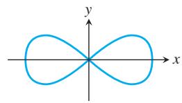
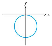
- Circle
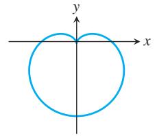
- Cardioid
-
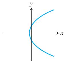
Parabola
-
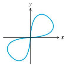
Lemniscate
Area in Polar Coordinates
Find the areas of the regions in the polar coordinate plane described in Exercises 47–50.
-
Enclosed by the limaçon
𝑟 = 2 − c o s 𝜃 -
Enclosed by one leaf of the three-leaved rose r = sin 3θ
-
Inside the “figure eight” r = +1 cos 2θ and outside the circle r = 1
-
Inside the cardioid
𝑟 = 2 ( 1 + s i n 𝜃 )
Length in Polar Coordinates
Find the lengths of the curves given by the polar coordinate equations in Exercises 51–54.
-
𝑟 = − 1 + c o s 𝜃 -
𝑟 = 2 s i n 𝜃 + 2 c o s 𝜃 , 0 ≤ 𝜃 ≤ 𝜋 / 2 -
𝑟 = 8 s i n 3 ( 𝜃 / 3 ) , 0 ≤ 𝜃 ≤ 𝜋 / 4 -
𝑟 = √ 1 + c o s 2 𝜃 , − 𝜋 / 2 ≤ 𝜃 ≤ 𝜋 / 2
Graphing Conic Sections
Sketch the parabolas in Exercises 55–58. Include the focus and directrix in each sketch.
-
𝑥 2 = − 4 𝑦 -
𝑥 2 = 2 𝑦
𝑦 2 = − ( 8 / 3 ) 𝑥
Find the eccentricities of the ellipses and hyperbolas in Exercises 59–62. Sketch each conic section. Include the foci, vertices, and asymptotes (as appropriate) in your sketch.
𝑥 2 + 2 𝑦 2 = 4
Exercises 63–68 give equations for conic sections and tell how many units up or down and to the right or left each curve is to be shifted. Find an equation for the new conic section, and find the new foci, vertices, centers, and asymptotes, as appropriate. If the curve is a parabola, find the new directrix as well.
-
𝑥 2 = − 1 2 𝑦 , -
𝑦 2 = 1 0 𝑥 , 1 / 2 , -
𝑥 2 9 + 𝑦 2 2 5 = 1 , -
𝑥 2 1 6 9 + 𝑦 2 1 4 4 = 1 , r i g h t 5 , u p 1 2
𝑥 2 3 6 − 𝑦 2 6 4 = 1 , l e f t 1 0 , d o w n 3
Identifying Conic Sections
Complete the squares to identify the conic sections in Exercises 69–76. Find their foci, vertices, centers, and asymptotes (as appropriate). If the curve is a parabola, find its directrix as well.
-
𝑥 2 − 4 𝑥 − 4 𝑦 2 = 0 -
4 𝑥 2 − 𝑦 2 + 4 𝑦 = 8 -
𝑦 2 − 2 𝑦 + 1 6 𝑥 = − 4 9 -
𝑥 2 − 2 𝑥 + 8 𝑦 = − 1 7 -
9 𝑥 2 + 1 6 𝑦 2 + 5 4 𝑥 − 6 4 𝑦 = − 1 -
2 5 𝑥 2 + 9 𝑦 2 − 1 0 0 𝑥 + 5 4 𝑦 = 4 4
Conics in Polar Coordinates
Sketch the conic sections whose polar coordinate equations are given in Exercises 77–80. Give polar coordinates for the vertices and, in the case of ellipses, for the centers as well.
𝑟 = 1 2 3 + s i n 𝜃
Exercises 81–84 give the eccentricities of conic sections with one focus at the origin of the polar coordinate plane, along with the directrix for that focus. Find a polar equation for each conic section.
-
𝑒 = 2 , 𝑟 c o s 𝜃 = 2 -
𝑒 = 1 , 𝑟 c o s 𝜃 = − 4 -
𝑒 = 1 / 2 , 𝑟 s i n 𝜃 = 2 -
𝑒 = 1 / 3 , 𝑟 s i n 𝜃 = − 6
Theory and Examples
-
Find the volume of the solid generated by revolving the region enclosed by the ellipse
9 𝑥 2 + 4 𝑦 2 = 3 6 -
The “triangular” region in the first quadrant bounded by the x-axis, the line
𝑥 = 4 , 9 𝑥 2 − 4 𝑦 2 = 3 6 -
Show that the equations x = = r y r cos , sin θ θ transform the polar equation
into the Cartesian equation
- Archimedes spirals The graph of an equation of the form
𝑟 = 𝑎 𝜃 .
CHAPTER 10 Additional and Advanced Exercises
Finding Conic Sections
-
Find an equation for the parabola with focus ( ) 4, 0 and directrix
𝑥 = 3 . -
Find the vertex, focus, and directrix of the parabola
-
Find an equation for the curve traced by the point
𝑃 ( 𝑥 , 𝑦 ) 𝑥 2 = 4 𝑦 -
A line segment of length a + b runs from the x-axis to the y-axis. The point P on the segment lies a units from one end and b units from the other end. Show that P traces an ellipse as the ends of the segment slide along the axes.
-
The vertices of an ellipse of eccentricity 0.5 lie at the points ( ) 0, 2 . Where do the foci lie?±
-
Find an equation for the ellipse of eccentricity 2 3 that has the line
𝑥 = 2 -
One focus of a hyperbola lies at the point
( 0 , − 7 ) 𝑦 = − 1 -
Find an equation for the hyperbola with foci ( ) 0, 2 and − ( ) 0, 2 that passes through the point ( ) 12, 7 .
-
Show that the line
is tangent to the ellipse
- Show that the line
is tangent to the hyperbola
Equations and Inequalities
What points in the xy-plane satisfy the equations and inequalities in Exercises 11–16? Draw a figure for each exercise.
-
( 𝑥 + 𝑦 ) ( 𝑥 2 + 𝑦 2 − 1 ) = 0 -
( 𝑥 2 / 9 ) + ( 𝑦 2 / 1 6 ) ≤ 1 -
( 𝑥 2 / 9 ) − ( 𝑦 2 / 1 6 ) ≤ 1 -
( 9 𝑥 2 + 4 𝑦 2 − 3 6 ) ( 4 𝑥 2 + 9 𝑦 2 − 1 6 ) ≤ 0 -
( 9 𝑥 2 + 4 𝑦 2 − 3 6 ) ( 4 𝑥 2 + 9 𝑦 2 − 1 6 ) > 0
Polar Coordinates
- a. Find an equation in polar coordinates for the curve
b. Find the length of the curve from
- Find the length of the curve
𝑟 = 2 s i n 3 ( 𝜃 / 3 ) , 0 ≤ 𝜃 ≤ 3 𝜋 ,
Exercises 19–22 give the eccentricities of conic sections with one focus at the origin of the polar coordinate plane, along with the directrix for that focus. Find a polar equation for each conic section.
Theory and Examples
- Epicycloids When a circle rolls externally along the circumference of a second, fixed circle, any point P on the circumference of the rolling circle describes an epicycloid, as shown here. Let the fixed circle have its center at the origin O and have radius a.
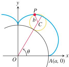
Let the radius of the rolling circle be b and let the initial position of the tracing point
- Find the centroid of the region enclosed by the x-axis and the cycloid arch
The Angle Between the Radius Vector and the Tangent Line to a Polar Coordinate Curve In Cartesian coordinates, when we want to discuss the direction of a curve at a point, we use the angle φ measured counterclockwise from the positive x-axis to the tangent line. In polar coordinates, it is more convenient to calculate the angle ψ from the radius vector to the tangent line (see the accompanying figure). The angle φ can then be calculated from the relation
which comes from applying the Exterior Angle Theorem to the triangle in the accompanying figure.
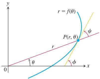
Suppose the equation of the curve is given in the form
are differentiable functions of θ with
Since
Furthermore,
because tan
Hence
The numerator in the last expression in Equation (4) is found from Equations (2) and (3) to be
Similarly, the denominator is
When we substitute these into Equation (4), we obtain
This is the equation we use for finding ψ as a function of θ.
- Show, by reference to a figure, that the angle
𝛽
When will the two curves intersect at right angles?
-
Find the value of tan ψ for the curve
𝑟 = s i n 4 ( 𝜃 / 4 ) -
Find the angle between the radius vector to the curve r a= 2 sin 3θ and its tangent when
𝜃 = 𝜋 / 6 -
a. Graph the hyperbolic spiralT
𝑟 𝜃 = 1
b. Confirm your finding in part (a) analytically.
-
The circles
𝑟 = √ 3 𝑟 = s i n 𝜃 ( √ 3 / 2 , 𝜋 / 3 ) -
Find the angle at which the cardioid
𝑟 = 𝑎 ( 1 − c o s 𝜃 ) 𝜃 = 𝜋 / 2
CHAPTER 10 Technology Application Projects
Mathematica/Maple Projects
Projects can be found within MyLab Math.
• Radar Tracking of a Moving Object
Part I: Convert from polar to Cartesian coordinates.
• Parametric and Polar Equations with a Figure Skater Part I: Visualize position, velocity, and acceleration to analyze motion defined by parametric equations. Part II: Find and analyze the equations of motion for a figure skater tracing a polar plot.