Chapter 4: Applications of Derivatives

OVERVIEW One of the most important applications of the derivative is its use as a tool for finding the optimal (best) solutions to problems. For example, what are the height and diameter of the cylinder of largest volume that can be inscribed in a given sphere? What are the dimensions of the strongest rectangular wooden beam that can be cut from a cylindrical log of given diameter? How many items should a manufacturer produce to maximize profit?
In this chapter we apply derivatives to find extreme values of functions, to determine and analyze the shapes of graphs, and to solve equations numerically. We also investigate how to recover a function from its derivative. The key to many of these applications is the Mean Value Theorem, which connects the derivative and the average change of a function.
4.1 Extreme Values of Functions on Closed Intervals
This section shows how to locate and identify extreme (maximum or minimum) values of a function from its derivative. Once we can do this, we can solve a variety of optimization problems (see Section 4.6). The domains of the functions we consider are intervals or unions of separate intervals.
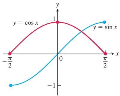
FIGURE 4.1 Absolute extrema for the sine and cosine functions on
DEFINITIONS Let
be a function with domain 𝑓 . Then 𝐷 has an absolute maximum value on 𝑓 at a point 𝐷 if 𝑐 𝑓 ( 𝑥 ) ≤ 𝑓 ( 𝑐 ) f o r a l l 𝑥 i n 𝐷 and an absolute minimum value on D at c if
𝑓 ( 𝑥 ) ≥ 𝑓 ( 𝑐 ) f o r a l l 𝑥 i n 𝐷 .
Maximum and minimum values are called extreme values of the function f. Absolute maxima or minima are also referred to as global maxima or minima.
For example, on the closed interval
Functions defined by the same equation or formula can have different extrema (maximum or minimum values), depending on the domain. A function might not have a maximum or minimum if the domain is unbounded or fails to contain an endpoint. We see this in the following example.
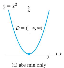
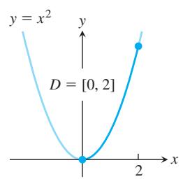
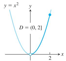
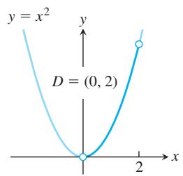
EXAMPLE 1 The absolute extrema of the following functions on their domains can be seen in Figure 4.2. Each function has the same defining equation,
| Function rule | Domain D | Absolute extrema on D |
| (a) | No absolute maximumAbsolute minimum of 0 at | |
| (b) | Absolute maximum of 4 at | |
| (c) | Absolute maximum of 4 at | |
| (d) | No absolute extrema |
(b) abs max and min
(c) abs max only
(d) no max or min
FIGURE 4.2 Graphs for Example 1.
HISTORICAL BIOGRAPHY
Daniel Bernoulli (1700–1789)
Daniel Bernoulli was the second son of mathematician Johann Bernoulli. In 1724, Bernoulli published his Exercitationes mathematicae that attracted considerable attention.
To know more, visit the companion Website.
Some of the functions in Example 1 do not have a maximum or a minimum value. The following theorem asserts that a function which is continuous over (or on) a finite closed interval
THEOREM 1 – The Extreme Value Theorem
If f is continuous on a closed interval
The proof of the Extreme Value Theorem requires a detailed knowledge of the real number system (see Appendix A.9) and we will not give it here. Figure 4.3 illustrates possible locations for the absolute extrema of a continuous function on a closed interval
The requirements in Theorem 1 that the interval be closed and finite, and that the function be continuous, are essential. Without them, the conclusion of the theorem need not hold. Example 1 shows that an absolute extreme value may not exist if the interval fails to be both closed and finite. The exponential function
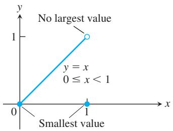
FIGURE 4.4 Even a single point of discontinuity can keep a function from having either a maximum or a minimum value on a closed interval. The function
is continuous at every point of
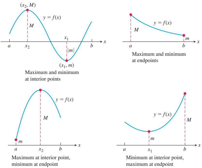
FIGURE 4.3 Some possibilities for a continuous function’s maximum and minimum on a closed interval
neither extreme value need exist on an infinite interval. Figure 4.4 shows that the continuity requirement cannot be omitted.
Local (Relative) Extreme Values
Figure 4.5 shows a graph with five points where a function has extreme values on its domain
DEFINITIONS A function f has a local maximum value at a point c within its domain D if
for all 𝑓 ( 𝑥 ) ≤ 𝑓 ( 𝑐 ) lying in some open interval containing c. 𝑥 ∈ 𝐷 A function f has a local minimum value at a point c within its domain D if
for all 𝑓 ( 𝑥 ) ≥ 𝑓 ( 𝑐 ) lying in some open interval containing c. 𝑥 ∈ 𝐷 If the domain of
is the closed interval 𝑓 , then [ 𝑎 , 𝑏 ] has a local maximum at the endpoint 𝑓 if 𝑥 = 𝑎 for all 𝑓 ( 𝑥 ) ≤ 𝑓 ( 𝑎 ) in some half-open interval 𝑥 . Likewise, [ 𝑎 , 𝑎 + 𝛿 ) , 𝛿 > 0 has a local maximum at an interior point 𝑓 if 𝑥 = 𝑐 for all 𝑓 ( 𝑥 ) ≤ 𝑓 ( 𝑐 ) in some open interval 𝑥 , and a local maximum at the endpoint ( 𝑐 − 𝛿 , 𝑐 + 𝛿 ) , 𝛿 > 0 if 𝑥 = 𝑏 for all 𝑓 ( 𝑥 ) ≤ 𝑓 ( 𝑏 ) in some half-open interval 𝑥 . The inequalities are reversed for local minimum values. In Figure 4.5, the function ( 𝑏 − 𝛿 , 𝑏 ] , 𝛿 > 0 has local maxima at 𝑓 and 𝑐 and local minima at 𝑑 , and 𝑎 , 𝑒 . Local extrema are also called relative extrema. Some functions can have infinitely many local extrema, even over a finite interval. One example is the function 𝑏 on the interval (0, 1]. (We graphed this function in Figure 2.41.) 𝑓 ( 𝑥 ) = s i n ( 1 / 𝑥 )
An absolute maximum is also a local maximum. Being the largest value overall, it is also the largest value in its immediate neighborhood. Hence, a list of all local maxima will automatically include the absolute maximum if there is one. Similarly, a list of all local minima will include the absolute minimum if there is one.
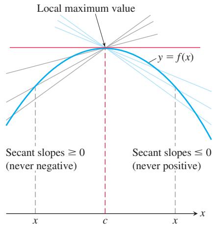
FIGURE 4.6 A curve with a local maximum value. The slope at c, simultaneously the limit of nonpositive numbers and nonnegative numbers, is zero.
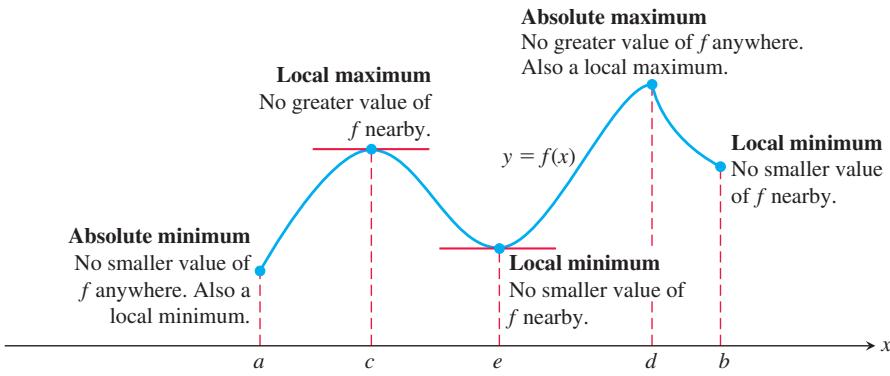
FIGURE 4.5 How to identify types of maxima and minima for a function with domain
Finding Extrema
The next theorem explains why we usually need to investigate only a few values to find a function’s extrema.
THEOREM 2—The First Derivative Theorem for Local Extreme Values
If f has a local maximum or minimum value at an interior point c of its domain, and if
Proof To prove that
To begin, suppose that
This means that the right-hand and left-hand limits both exist at
Similarly,
Together, Equations (1) and (2) imply
This proves the theorem for local maximum values. To prove it for local minimum values, we simply use
(a)
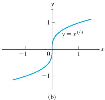
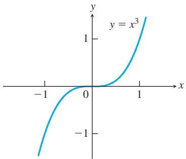
FIGURE 4.7 Critical points without extreme values. (a)
(b)
Theorem 2 says that a function’s first derivative is always zero at an interior point where the function has a local extreme value and the derivative is defined. If we recall that all the domains we consider are intervals or unions of separate intervals, the only places where a function
- interior points where
𝑓 ′ = 0
- interior points where
𝑓 ′
At
- endpoints of an interval in the domain of
𝑓 𝑥 = 𝑎 𝑥 = 𝑏
The following definition helps us to summarize these results.
DEFINITION An interior point of the domain of a function
where 𝑓 is zero or undefined is a critical point of 𝑓 ′ . 𝑓
Thus the only domain points where a continuous function on a closed and finite interval can assume extreme values are critical points and endpoints. However, be careful not to misinterpret what is being said here. A function may have a critical point at x = c without having a local extreme value there. For instance, both of the functions
If the interval is not closed or not finite (such as a < x < b or a < x <
Finding the Absolute Extrema of a Continuous Function f on a Finite Closed Interval
-
Find all critical points of
𝑓 -
Evaluate f at all critical points and endpoints.
-
Take the largest and smallest of these values.
EXAMPLE 2 Find the absolute maximum and minimum values of
Solution The function is differentiable over its entire domain, so the only critical point occurs where
Critical point value:
Endpoint values:
The function has an absolute maximum value of 4 at x = -2 and an absolute minimum value of 0 at x = 0.
EXAMPLE 3 Find the absolute maximum and minimum values of
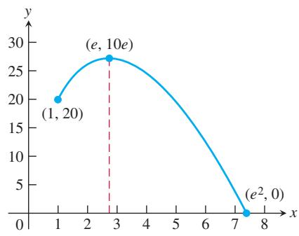
FIGURE 4.8 The extreme values of
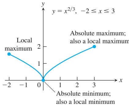
FIGURE 4.9 The extreme values of
Solution Figure 4.8 suggests that
We evaluate the function at the critical points and endpoints and take the largest and smallest of the resulting values.
The first derivative is
The only critical point in the domain
Critical point value:
Endpoint values:
We can see from this list that the function’s absolute maximum value is
EXAMPLE 4 Find the absolute maximum and minimum values of
Solution We evaluate the function at the critical points and endpoints and take the largest and smallest of the resulting values.
The first derivative,
has no zeros but is undefined at the interior point x = 0. The values of f at this one critical point and at the endpoints are
Critical point value:
Endpoint values:
We can see from this list that the function’s absolute maximum value is
Theorem 1 leads to a method for finding the absolute maxima and absolute minima of a differentiable function on a finite closed interval. On more general domains, such as
EXERCISES 4.1
Finding Extrema from Graphs
In Exercises 1–6, determine from the graph whether the function has any absolute extreme values on
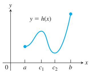
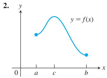
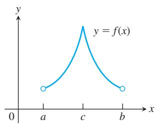
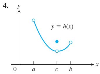
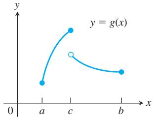
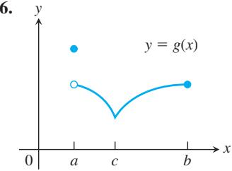
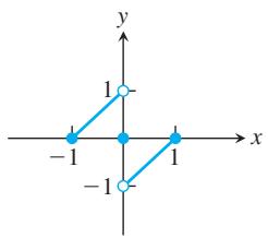
In Exercises 7–10, find the absolute extreme values and where they occur.
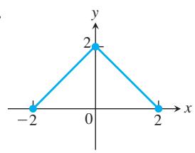
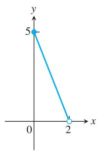
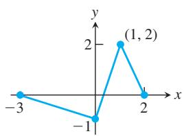
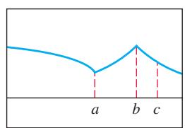
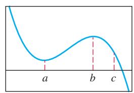
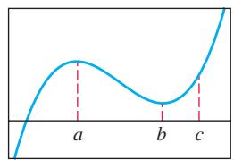
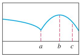
In Exercises 11–14, match the table with a graph.
| 11. x | |
| a | 0 |
| b | 0 |
| c | 5 |
| 12. x | |
| a | 0 |
| b | 0 |
| c | -5 |
| 14. x | |
| a | does not exist |
| b | does not exist |
| c | -1.7 |
| a | does not exist |
| b | 0 |
| c | -2 |
(a)
(c)
(b)
(d)
In Exercises 15–20, sketch the graph of each function and determine whether the function has any absolute extreme values on its domain. Explain how your answer is consistent with Theorem 1.
Absolute Extrema on Finite Closed Intervals
In Exercises 21–36, find the absolute maximum and minimum values of each function on the given interval. Then graph the function. Identify the points on the graph where the absolute extrema occur, and include their coordinates.
-
𝑓 ( 𝑥 ) = 2 3 𝑥 − 5 , − 2 ≤ 𝑥 ≤ 3 -
𝑓 ( 𝑥 ) = − 𝑥 − 4 , − 4 ≤ 𝑥 ≤ 1 -
𝑓 ( 𝑥 ) = 𝑥 2 − 1 , − 1 ≤ 𝑥 ≤ 2 -
𝑓 ( 𝑥 ) = 4 − 𝑥 3 , − 2 ≤ 𝑥 ≤ 1 -
𝐹 ( 𝑥 ) = − 1 𝑥 2 , 0 . 5 ≤ 𝑥 ≤ 2 -
𝐹 ( 𝑥 ) = − 1 𝑥 , − 2 ≤ 𝑥 ≤ − 1 -
ℎ ( 𝑥 ) = 3 √ 𝑥 , − 1 ≤ 𝑥 ≤ 8 -
ℎ ( 𝑥 ) = − 3 𝑥 2 / 3 , − 1 ≤ 𝑥 ≤ 1 -
𝑔 ( 𝑥 ) = √ 4 − 𝑥 2 , − 2 ≤ 𝑥 ≤ 1 -
𝑔 ( 𝑥 ) = − √ 5 − 𝑥 2 , − √ 5 ≤ 𝑥 ≤ 0 -
𝑓 ( 𝜃 ) = s i n 𝜃 , − 𝜋 2 ≤ 𝜃 ≤ 5 𝜋 6 -
𝑓 ( 𝜃 ) = t a n 𝜃 , − 𝜋 3 ≤ 𝜃 ≤ 𝜋 4 -
𝑔 ( 𝑥 ) = c s c 𝑥 , 𝜋 3 ≤ 𝑥 ≤ 2 𝜋 3 -
𝑔 ( 𝑥 ) = s e c 𝑥 , − 𝜋 3 ≤ 𝑥 ≤ 𝜋 6 -
𝑓 ( 𝑡 ) = 2 − | 𝑡 | , − 1 ≤ 𝑡 ≤ 3 -
𝑓 ( 𝑡 ) = | 𝑡 − 5 | 4 ≤ 𝑡 ≤ 7
In Exercises 37–40:
a. Find the absolute maximum and minimum values of each function on the given interval.
T b. Graph the function, identify the points on the graph where the absolute extrema occur, and include their coordinates.
-
𝑔 ( 𝑥 ) = 𝑥 𝑒 − 𝑥 , − 1 ≤ 𝑥 ≤ 1 -
ℎ ( 𝑥 ) = l n ( 𝑥 + 1 ) − 𝑥 2 , 0 ≤ 𝑥 ≤ 3 -
𝑓 ( 𝑥 ) = 1 𝑥 + l n 𝑥 , 0 . 5 ≤ 𝑥 ≤ 4 -
𝑔 ( 𝑥 ) = 𝑒 − 𝑥 2 , − 2 ≤ 𝑥 ≤ 1
In Exercises 41–44, find the function’s absolute maximum and minimum values and say where they occur.
-
𝑓 ( 𝑥 ) = 𝑥 4 / 3 , − 1 ≤ 𝑥 ≤ 8 -
𝑓 ( 𝑥 ) = 𝑥 5 / 3 , − 1 ≤ 𝑥 ≤ 8 -
𝑔 ( 𝜃 ) = 𝜃 3 / 5 , − 3 2 ≤ 𝜃 ≤ 1 -
ℎ ( 𝜃 ) = 3 𝜃 2 / 3 , − 2 7 ≤ 𝜃 ≤ 8
Finding Critical Points
In Exercises 45–56, determine all critical points and all domain endpoints for each function.
-
𝑦 = 𝑥 2 − 6 𝑥 + 7 -
𝑓 ( 𝑥 ) = 6 𝑥 2 − 𝑥 3 -
𝑓 ( 𝑥 ) = 𝑥 ( 4 − 𝑥 ) 3 4 8 . 𝑔 ( 𝑥 ) = ( 𝑥 − 1 ) 2 ( 𝑥 − 3 ) 2 -
𝑦 = 𝑥 2 + 2 𝑥 -
𝑓 ( 𝑥 ) = 𝑥 2 𝑥 − 2 -
𝑦 = 𝑥 2 − 3 2 √ 𝑥 -
𝑔 ( 𝑥 ) = √ 2 𝑥 − 𝑥 2 -
𝑦 = l n ( 𝑥 + 1 ) − t a n − 1 𝑥 -
𝑦 = 2 √ 1 − 𝑥 2 + a r c s i n 𝑥 -
𝑦 = 𝑥 3 + 3 𝑥 2 − 2 4 𝑥 + 7 -
𝑦 = 𝑥 − 3 𝑥 2 / 3
Theory and Examples
In Exercises 57 and 58, give reasons for your answers.
- Let
𝑓 ( 𝑥 ) = ( 𝑥 − 2 ) 2 / 3
a. Does
b. Show that the only local extreme value of f occurs at x = 2.
c. Does the result in part (b) contradict the Extreme Value Theorem?
d. Repeat parts (a) and (b) for
- Let
𝑓 ( 𝑥 ) = | 𝑥 3 − 9 𝑥 |
a. Does
b. Does
c. Does
d. Determine all extrema of
In Exercises 59–62, show that the function has neither an absolute minimum nor an absolute maximum on its natural domain.
-
𝑦 = 𝑥 1 1 + 𝑥 3 + 𝑥 − 5 -
𝑦 = 3 𝑥 + t a n 𝑥 -
𝑦 = 1 − 𝑒 𝑥 𝑒 𝑥 + 1 -
𝑦 = 2 𝑥 − s i n 2 𝑥 -
A minimum with no derivative The function
𝑓 ( 𝑥 ) = | 𝑥 | 𝑥 = 0 𝑓 𝑥 = 0 -
Even functions If an even function
𝑓 ( 𝑥 ) -
Odd functions If an odd function
𝑔 ( 𝑥 ) -
No critical points or endpoints exist We know how to find the extreme values of a continuous function
𝑓 ( 𝑥 ) -
The function
models the volume of a box.
a. Find the extreme values of V.
b. Interpret any values found in part (a) in terms of the volume of the box.
- Cubic functions Consider the cubic function
a. Show that
b. How many local extreme values can
- Maximum height of a vertically moving body The height of a body moving vertically is given by
with
- Peak alternating current Suppose that at any given time t (in seconds) the current i (in amperes) in an alternating current circuit is
𝑖 = 2 c o s 𝑡 + 2 s i n 𝑡
T Graph the functions in Exercises 71–74. Then find the extreme values of the function on the interval and say where they occur.
-
𝑓 ( 𝑥 ) = | 𝑥 − 2 | + | 𝑥 + 3 | , − 5 ≤ 𝑥 ≤ 5 -
𝑔 ( 𝑥 ) = | 𝑥 − 1 | − | 𝑥 − 5 | , − 2 ≤ 𝑥 ≤ 7 -
ℎ ( 𝑥 ) = | 𝑥 + 2 | − | 𝑥 − 3 | − ∞ < 𝑥 < ∞ -
𝑘 ( 𝑥 ) = | 𝑥 + 1 | + | 𝑥 − 3 | − ∞ < 𝑥 < ∞
COMPUTER EXPLORATIONS
In Exercises 75–82, you will use a CAS to help find the absolute extrema of the given function over the specified closed interval. Perform the following steps.
a. Plot the function over the interval to see its general behavior there.
b. Find the interior points where
c. Find the interior points where
d. Evaluate the function at all points found in parts (b) and (c) and at the endpoints of the interval.
e. Find the function’s absolute extreme values on the interval and identify where they occur.
-
𝑓 ( 𝑥 ) = 𝑥 4 − 8 𝑥 2 + 4 𝑥 + 2 , [ − 2 0 / 2 5 , 6 4 / 2 5 ] -
𝑓 ( 𝑥 ) = − 𝑥 4 + 4 𝑥 3 − 4 𝑥 + 1 , [ − 3 / 4 , 3 ] -
𝑓 ( 𝑥 ) = 𝑥 2 / 3 ( 3 − 𝑥 ) , [ − 2 , 2 ] -
𝑓 ( 𝑥 ) = 2 + 2 𝑥 − 3 𝑥 2 / 3 , [ − 1 , 1 0 / 3 ] -
𝑓 ( 𝑥 ) = √ 𝑥 + c o s 𝑥 , [ 0 , 2 𝜋 ] -
𝑓 ( 𝑥 ) = 𝑥 3 / 4 − s i n 𝑥 + 1 2 , [ 0 , 2 𝜋 ] -
𝑓 ( 𝑥 ) = 𝜋 𝑥 2 𝑒 − 3 𝑥 / 2 , [ 0 , 5 ] -
𝑓 ( 𝑥 ) = l n ( 2 𝑥 + 𝑥 s i n 𝑥 ) , [ 1 , 1 5 ]
4.2 The Mean Value Theorem
(a)
We know that constant functions have zero derivatives, but could there be a more complicated function whose derivative is always zero? If two functions have identical derivatives over an interval, how are the functions related? We answer these and other questions in this chapter by applying the Mean Value Theorem. First we introduce a special case, known as Rolle’s Theorem, which is used to prove the Mean Value Theorem.
(b)
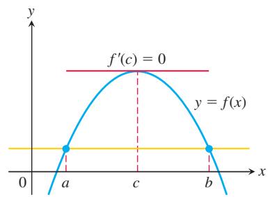
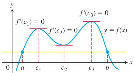
FIGURE 4.10 Rolle’s Theorem says that a differentiable curve has at least one horizontal tangent between any two points where it crosses a horizontal line. It may have just one (a), or it may have more (b).
Rolle’s Theorem
As suggested by its graph, if a differentiable function crosses a horizontal line at two different points, there is at least one point between them where the tangent to the graph is horizontal and the derivative is zero (Figure 4.10). We now state and prove this result.
THEOREM 3—Rolle’s Theorem
Suppose that
Proof Being continuous,
-
at interior points where
𝑓 ′ -
at interior points where
𝑓 ′ -
at endpoints of the interval, in this case a and b.
HISTORICAL BIOGRAPHY
(1652-1719)
French mathematician Michel Rolle was largely self-educated in mathematics. He worked as an accountant and studied algebra and the Diophantine equations whenever he found time.
To know more, visit the companion Website.
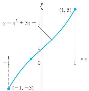
FIGURE 4.12 The only real zero of the polynomial
By hypothesis, f has a derivative at every interior point. That rules out possibility (2), leaving us with interior points where
If either the maximum or the minimum occurs at a point
If both the absolute maximum and the absolute minimum occur at the endpoints, then because
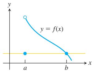
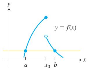
The hypotheses of Theorem 3 are essential. If they fail at even one point, the graph may not have a horizontal tangent (Figure 4.11).
(a) Discontinuous at an endpoint of
(b) Discontinuous at an interior point of
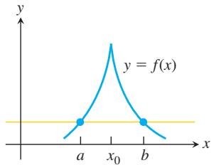
(c) Continuous on
FIGURE 4.11 There may be no horizontal tangent line if the hypotheses of Rolle’s Theorem do not hold.
Rolle’s Theorem may be combined with the Intermediate Value Theorem to show when there is only one real solution of an equation
EXAMPLE 1 Show that the equation
has exactly one real solution.
Solution We define the continuous function
Since
is never zero (because it is always positive). Therefore,
Tangent line parallel to secant line
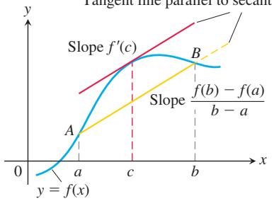
FIGURE 4.13 Geometrically, the Mean Value Theorem says that somewhere between a and b the curve has at least one tangent line parallel to the secant line that joins A and B.
HISTORICAL BIOGRAPHY Joseph-Louis Lagrange (1736–1813)
Lagrange was born in Turin, Italy. He enjoyed studying mathematics, despite his father’s wish that he study law. Lagrange’s mathematical contributions began as early as 1754 with the discovery of the calculus of variations and continued with applications to mechanics in 1756.
To know more, visit the companion Website.
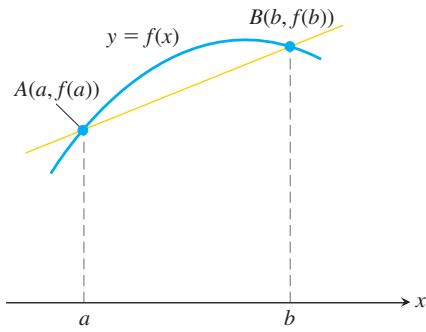
FIGURE 4.14 The graph of f and the secant line AB over the interval [a, b].
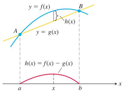
FIGURE 4.15 The secant line AB is the graph of the function
The Mean Value Theorem
The Mean Value Theorem, which was first stated by Joseph-Louis Lagrange, is a slanted version of Rolle’s Theorem (Figure 4.13). The Mean Value Theorem guarantees that there is a point where the tangent line is parallel to the secant line that joins
THEOREM 4—The Mean Value Theorem
Suppose
Proof We picture the graph of f and draw a line through the points
(point-slope equation). The vertical difference between the graphs of
Figure 4.15 shows the graphs of
The function
To verify Equation (1), we differentiate both sides of Equation (3) with respect to x and then set x = c:
which is what we set out to prove.
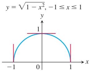
FIGURE 4.16 The function
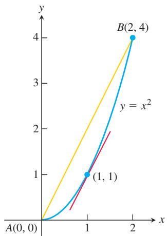
FIGURE 4.17 As we find in Example 1, c = 1 is where the tangent line is parallel to the secant line.
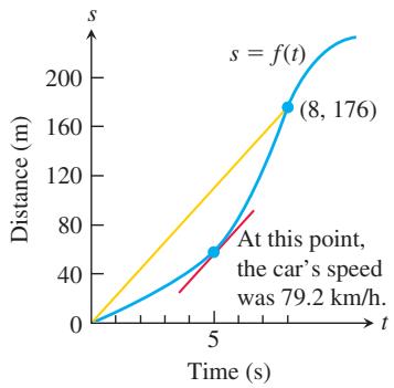
FIGURE 4.18 Distance versus elapsed time for the car in Example 3.
The hypotheses of the Mean Value Theorem do not require f to be differentiable at either a or b. One-sided continuity at a and b is enough (Figure 4.16).
EXAMPLE 2 The function
A Physical Interpretation
We can think of the number
EXAMPLE 3 If a car accelerating from zero takes 8 s to go 176 m, its average velocity for the 8-s interval is
Mathematical Consequences
At the beginning of the section, we asked what kind of function has a zero derivative over an interval. The first corollary of the Mean Value Theorem provides the answer that only constant functions have zero derivatives.
COROLLARY 1 If
Proof We want to show that f has a constant value on the interval
at some point
At the beginning of this section, we also asked about the relationship between two functions that have identical derivatives over an interval. The next corollary tells us that their values on the interval have a constant difference.
COROLLARY 2 If
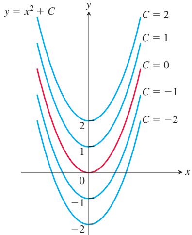
FIGURE 4.19 From a geometric point of view, Corollary 2 of the Mean Value Theorem says that the graphs of functions with identical derivatives on an interval can differ only by a vertical shift. The graphs of the functions with derivative 2x are the parabolas
Proof At each point
Thus,
Corollaries 1 and 2 are also true if the open interval
Corollary 2 will play an important role when we discuss antiderivatives in Section 4.8. It tells us, for instance, that since the derivative of
EXAMPLE 4 Find the function
Solution Since the derivative of
The function is
Finding Velocity and Position from Acceleration
We can use Corollary 2 to find the velocity and position functions of an object moving along a vertical line. Assume the object or body is falling freely from rest with acceleration
We know that the velocity
for some constant C. Since the body falls from rest,
The velocity function must be
We know that
for some constant C. Since
The position function is
The ability to find functions from their rates of change is one of the very powerful tools of calculus. As we will see, it lies at the heart of the mathematical developments in Chapter 5.
EXERCISES 4.2
Checking the Mean Value Theorem
Find the value or values of c that satisfy the equation
in the conclusion of the Mean Value Theorem for the functions and intervals in Exercises 1–8.
-
𝑓 ( 𝑥 ) = 𝑥 2 + 2 𝑥 − 1 , [ 0 , 1 ] 𝟐 . 𝑓 ( 𝑥 ) = 𝑥 2 / 3 , [ 0 , 1 ] -
𝑓 ( 𝑥 ) = 𝑥 + 1 𝑥 , [ 1 2 , 2 ] 𝟒 . 𝑓 ( 𝑥 ) = √ 𝑥 − 1 , [ 1 , 3 ] -
𝑓 ( 𝑥 ) = a r c s i n 𝑥 , [ − 1 , 1 ] -
𝑓 ( 𝑥 ) = l n ( 𝑥 − 1 ) , [ 2 , 4 ] -
𝑓 ( 𝑥 ) = 𝑥 3 − 𝑥 2 , [ − 1 , 2 ] -
𝑔 ( 𝑥 ) = { 𝑥 3 , − 2 ≤ 𝑥 ≤ 0 𝑥 2 , 0 < 𝑥 ≤ 2
Which of the functions in Exercises 9–14 satisfy the hypotheses of the Mean Value Theorem on the given interval, and which do not? Give reasons for your answers.
-
𝑓 ( 𝑥 ) = 𝑥 2 / 3 , [ − 1 , 8 ] -
𝑓 ( 𝑥 ) = 𝑥 4 / 5 , [ 0 , 1 ] -
𝑓 ( 𝑥 ) = √ 𝑥 ( 1 − 𝑥 ) , [ 0 , 1 ] -
𝑓 ( 𝑥 ) = { s i n 𝑥 𝑥 , − 𝜋 ≤ 𝑥 < 0 0 , 𝑥 = 0 -
𝑓 ( 𝑥 ) = { 𝑥 2 − 𝑥 , − 2 ≤ 𝑥 ≤ − 1 2 𝑥 2 − 3 𝑥 − 3 , − 1 < 𝑥 ≤ 0 -
𝑓 ( 𝑥 ) = { 2 𝑥 − 3 , 0 ≤ 𝑥 ≤ 2 6 𝑥 − 𝑥 2 − 7 , 2 < 𝑥 ≤ 3 -
The function
is zero at
- For what values of a, m, and b does the function
satisfy the hypotheses of the Mean Value Theorem on the interval [0, 2]?
Roots (Zeros)
- a. Plot the zeros of each polynomial on a line together with the zeros of its first derivative.
i)
iii)
iv)
b. Use Rolle’s Theorem to prove that between every two zeros of
-
Suppose that
𝑓 ″ [ 𝑎 , 𝑏 ] 𝑓 𝑓 ″ ( 𝑎 , 𝑏 ) -
Show that if
𝑓 ″ > 0 [ 𝑎 , 𝑏 ] 𝑓 ′ [ 𝑎 , 𝑏 ] 𝑓 ″ < 0 [ 𝑎 , 𝑏 ] -
Show that a cubic polynomial can have at most three real zeros.
Show that the functions in Exercises 21–28 have exactly one zero in the given interval.
-
𝑓 ( 𝑥 ) = 𝑥 4 + 3 𝑥 + 1 , [ − 2 , − 1 ] -
𝑓 ( 𝑥 ) = 𝑥 3 + 4 𝑥 2 + 7 , ( − ∞ , 0 ) -
𝑔 ( 𝑡 ) = √ 𝑡 + √ 1 + 𝑡 − 4 , ( 0 , ∞ ) -
𝑔 ( 𝑡 ) = 1 1 − 𝑡 + √ 1 + 𝑡 − 3 . 1 , ( − 1 , 1 ) -
𝑟 ( 𝜃 ) = 𝜃 + s i n 2 ( 𝜃 3 ) − 8 , ( − ∞ , ∞ ) -
𝑟 ( 𝜃 ) = 2 𝜃 − c o s 2 𝜃 + √ 2 , ( − ∞ , ∞ ) -
𝑟 ( 𝜃 ) = s e c 2 𝜃 − c o s ( 2 𝜃 ) − 1 , ( 0 , 𝜋 / 2 ) -
𝑟 ( 𝜃 ) = 3 t a n 𝜃 − c o t 𝜃 − 𝜃 , ( 0 , 𝜋 / 2 )
Finding Functions from Derivatives
-
Suppose that
𝑓 ( − 1 ) = 3 𝑓 ′ ( 𝑥 ) = 0 𝑥 𝑓 ( 𝑥 ) = 3 𝑥 -
Suppose that
𝑓 ( 0 ) = 5 𝑓 ′ ( 𝑥 ) = 2 𝑓 ( 𝑥 ) = 2 𝑥 + 5 -
Suppose that
𝑓 ′ ( 𝑥 ) = 2 𝑥 𝑥 𝑓 ( 2 )
a.
- What can be said about functions whose derivatives are constant? Give reasons for your answer.
In Exercises 33–38, find all possible functions with the given derivative.
-
a.
𝑦 ′ = 𝑥 𝑦 ′ = 𝑥 2 𝑦 ′ = 𝑥 3 -
a.
𝑦 ′ = 2 𝑥 𝑦 ′ = 2 𝑥 − 1 𝑦 ′ = 3 𝑥 2 + 2 𝑥 − 1 -
a.
𝑦 ′ = − 1 𝑥 2 𝑦 ′ = 1 − 1 𝑥 2 𝑦 ′ = 5 + 1 𝑥 2 -
a.
𝑦 ′ = 1 2 √ 𝑥 𝑦 ′ = 1 √ 𝑥 𝑦 ′ = 4 𝑥 − 1 √ 𝑥 -
a.
𝑦 ′ = s i n 2 𝑡 𝑦 ′ = c o s 𝑡 2 𝑦 ′ = s i n 2 𝑡 + c o s 𝑡 2 -
a.
𝑦 ′ = s e c 2 𝜃 𝑦 ′ = √ 𝜃 𝑦 ′ = √ 𝜃 − s e c 2 𝜃
In Exercises 39–42, find the function with the given derivative whose graph passes through the point P.
-
𝑓 ′ ( 𝑥 ) = 2 𝑥 − 1 , 𝑃 ( 0 , 0 ) -
𝑔 ′ ( 𝑥 ) = 1 𝑥 2 + 2 𝑥 , 𝑃 ( − 1 , 1 ) -
𝑓 ′ ( 𝑥 ) = 𝑒 2 𝑥 , 𝑃 ( 0 , 3 2 ) -
𝑟 ′ ( 𝑡 ) = s e c 𝑡 t a n 𝑡 − 1 , 𝑃 ( 0 , 0 )
Finding Position from Velocity or Acceleration
Exercises 43–46 give the velocity v = ds/dt and initial position of an object moving along a coordinate line. Find the object’s position at time t.
-
𝑣 = 9 . 8 𝑡 + 5 , 𝑠 ( 0 ) = 1 0 -
𝑣 = 3 2 𝑡 − 2 , 𝑠 ( 0 . 5 ) = 4 -
𝑣 = s i n 𝜋 𝑡 , 𝑠 ( 0 ) = 0 -
𝑣 = 2 𝜋 c o s 2 𝑡 𝜋 , 𝑠 ( 𝜋 2 ) = 1
Exercises 47–50 give the acceleration
-
𝑎 = 𝑒 𝑡 𝜐 ( 0 ) = 2 0 𝑠 ( 0 ) = 5 -
𝑎 = 9 . 8 , 𝑣 ( 0 ) = − 3 , 𝑠 ( 0 ) = 0 -
𝑎 = − 4 s i n 2 𝑡 , 𝑣 ( 0 ) = 2 , 𝑠 ( 0 ) = − 3 -
𝑎 = 9 𝜋 2 c o s 3 𝑡 𝜋 𝑣 ( 0 ) = 0 𝑠 ( 0 ) = − 1
Applications
-
Temperature change It took 14 s for a mercury thermometer to rise from
− 1 9 ∘ 𝐶 1 0 0 ∘ 𝐶 8 . 5 ∘ 𝐶 / 𝑠 -
A trucker handed in a ticket at a tollbooth showing that in 2 hours she had covered 230 km on a toll road with speed limit 100 km/h. The trucker was cited for speeding. Why?
-
Classical accounts tell us that a 170-oar trireme (ancient Greek or Roman warship) once covered 184 sea miles in 24 hours. Explain why at some point during this feat the trireme’s speed exceeded 7.5 knots (sea or nautical miles per hour).
-
A marathoner ran the 42-km New York City Marathon in 2.2 hours. Show that at least twice the marathoner was running at exactly 18 km/h, assuming the initial and final speeds are zero.
-
Show that at some instant during a 2-hour automobile trip the car’s speedometer reading will equal the average speed for the trip.
-
Free fall on the moon On our moon, the acceleration of gravity is
1 . 6 𝑚 / 𝑠 2
Theory and Examples
-
The geometric mean of a and b The geometric mean of two positive numbers a and b is the number
√ 𝑎 𝑏 𝑓 ( 𝑥 ) = 1 / 𝑥 [ 𝑎 , 𝑏 ] 𝑐 = √ 𝑎 𝑏 -
The arithmetic mean of
𝑎 𝑏 𝑎 𝑏 ( 𝑎 + 𝑏 ) / 2 𝑐 𝑓 ( 𝑥 ) = 𝑥 2 [ 𝑎 , 𝑏 ] 𝑐 = ( 𝑎 + 𝑏 ) / 2
T 59. Graph the function
What does the graph do? Why does the function behave this way? Give reasons for your answers.
- Rolle’s Theorem
a. Construct a polynomial
b. Graph
c. Do
-
Unique solution Assume that
𝑓 [ 𝑎 , 𝑏 ] ( 𝑎 , 𝑏 ) 𝑓 ( 𝑎 ) 𝑓 ( 𝑏 ) 𝑓 ′ ≠ 0 𝑎 𝑏 𝑓 ( 𝑥 ) = 0 𝑎 𝑏 -
Parallel tangent line Assume that
𝑓 𝑔 [ 𝑎 , 𝑏 ] 𝑓 ( 𝑎 ) = 𝑔 ( 𝑎 ) 𝑓 ( 𝑏 ) = 𝑔 ( 𝑏 ) 𝑎 𝑏 𝑓 𝑔 -
Suppose that
𝑓 ′ ( 𝑥 ) ≤ 1 1 ≤ 𝑥 ≤ 4 𝑓 ( 4 ) − 𝑓 ( 1 ) ≤ 3 -
Suppose that
0 < 𝑓 ′ ( 𝑥 ) < 1 / 2 𝑥 𝑓 ( − 1 ) < 𝑓 ( 1 ) < 2 + 𝑓 ( − 1 ) -
Show that
| c o s 𝑥 − 1 | ≤ | 𝑥 | 𝑥 𝑓 ( 𝑡 ) = c o s 𝑡 𝑥 -
Show that for any numbers
𝑎 𝑏 | s i n 𝑏 − s i n 𝑎 | ≤ | 𝑏 − 𝑎 | -
If the graphs of two differentiable functions
𝑓 ( 𝑥 ) 𝑔 ( 𝑥 ) -
If
| 𝑓 ( 𝑤 ) − 𝑓 ( 𝑥 ) | ≤ | 𝑤 − 𝑥 | 𝑤 𝑥 𝑓 − 1 ≤ 𝑓 ′ ( 𝑥 ) ≤ 1 𝑥 -
Assume that
𝑓 𝑎 ≤ 𝑥 ≤ 𝑏 𝑓 ( 𝑏 ) < 𝑓 ( 𝑎 ) 𝑓 ′ 𝑎 𝑏 -
Let f be a function defined on an interval
[ 𝑎 , 𝑏 ]
where
T 71. Use the inequalities in Exercise 70 to estimate
T 72. Use the inequalities in Exercise 70 to estimate
- Let
𝑓 𝑥 𝑓 ( 1 ) = 1 𝑓 ′ < 0 ( − ∞ , 1 ) 𝑓 ′ > 0 ( 1 , ∞ )
a. Show that𝑓 ( 𝑥 ) ≥ 1 𝑥
b. Must
- Let
𝑓 ( 𝑥 ) = 𝑝 𝑥 2 + 𝑞 𝑥 + 𝑟 [ 𝑎 , 𝑏 ] 𝑐 ( 𝑎 , 𝑏 ) 𝑓
4.3 Monotonic Functions and the First Derivative Test
In sketching the graph of a differentiable function, it is useful to know where it increases (rises from left to right) and where it decreases (falls from left to right) over an interval. This section gives a test to determine where it increases and where it decreases. We also show how to test the critical points of a function to identify whether local extreme values are present.
Increasing Functions and Decreasing Functions
As another corollary to the Mean Value Theorem, we show that functions with positive derivatives are increasing functions and functions with negative derivatives are decreasing functions. A function that is either increasing on an interval or decreasing on an interval is said to be monotonic on the interval.
COROLLARY 3 Suppose that
Proof Let
for some c between
Corollary 3 tells us that
To find the intervals where a function
EXAMPLE 1 Find the critical points of
Solution The function
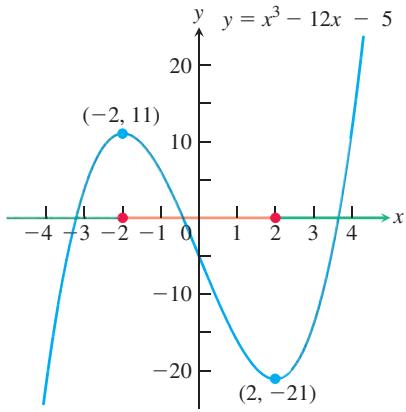
FIGURE 4.20 The function
HISTORICAL BIOGRAPHY Edmund Halley (1656–1742)
Halley, a British biologist, geologist, sea captain, astronomer, and mathematician, encouraged Newton to write the Principia. Despite all of Halley’s accomplishments, he is known today as the man who calculated the orbit of the comet of 1682.
To know more, visit the companion Website.
is zero at x = -2 and x = 2. These critical points subdivide the domain of f to create nonoverlapping open intervals
| Interval | |||
| Sign of | + | - | + |
| Behavior of | increasing | decreasing | increasing |
We used “strict” less-than inequalities to identify the intervals in the summary table for Example 1, since open intervals were specified. Corollary 3 says that we could use
First Derivative Test for Local Extrema
In Figure 4.21, at the points where f has a minimum value,
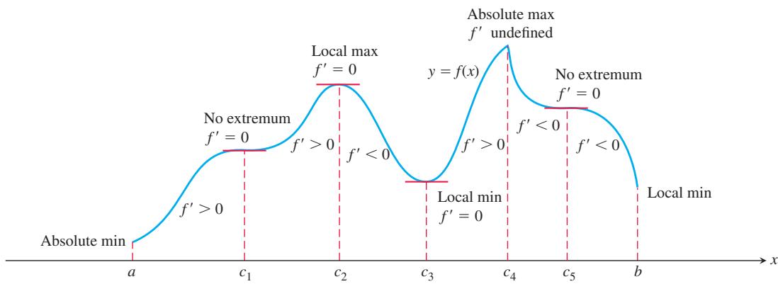
FIGURE 4.21 The critical points of a function locate where it is increasing and where it is decreasing. The first derivative changes sign at a critical point where a local extremum occurs.
These observations lead to a test for the presence and nature of local extreme values of differentiable functions.
First Derivative Test for Local Extrema
Suppose that c is a critical point of a continuous function f, and that f is differentiable at every point in some interval containing c except possibly at c itself. Moving across this interval from left to right,
-
if
𝑓 ′ -
if
𝑓 ′ -
if
𝑓 ′ 𝑓 ′
The test for local extrema at endpoints is similar, but there is only one side to consider in determining whether
Proof of the First Derivative Test Part (1). Since the sign of
Parts (2) and (3) are proved similarly.
EXAMPLE 2 Find the critical points of
Identify the open intervals on which
Solution The function f is continuous at all x since it is the product of two continuous functions,
is zero at
The critical points partition the x-axis into open intervals on which
| Interval | x < 0 | 0 < x < 1 | x > 1 |
| Sign of f' | - | - | + |
| Behavior of f | decreasing | decreasing | increasing |
Corollary 3 to the Mean Value Theorem implies that f decreases on
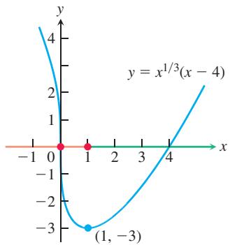
FIGURE 4.22 The function
The value of the local minimum is
Note that
EXAMPLE 3 Find the critical points of
Identify the open intervals on which
Solution The function
Using the Derivative Product Rule, we find the derivative
Since
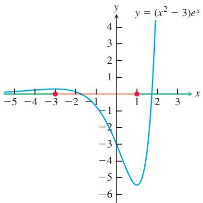
FIGURE 4.23 The graph of
The zeros x = -3 and x = 1 partition the x-axis into open intervals as follows.
| Interval | x < -3 | -3 < x < 1 | 1 < x |
| Sign of f' | + | - | + |
| Behavior of f | increasing | decreasing | increasing |
We can see from the table that there is a local maximum (about 0.299) at
EXERCISES 4.3
Analyzing Functions from Derivatives
Answer the following questions about the functions whose derivatives are given in Exercises 1–14:
a. What are the critical points of
b. On what open intervals is f increasing or decreasing?
c. At what points, if any, does f assume local maximum or minimum values?
-
𝑓 ′ ( 𝑥 ) = 𝑥 ( 𝑥 − 1 ) -
𝑓 ′ ( 𝑥 ) = ( 𝑥 − 1 ) ( 𝑥 + 2 ) -
𝑓 ′ ( 𝑥 ) = ( 𝑥 − 1 ) 2 ( 𝑥 + 2 ) -
𝑓 ′ ( 𝑥 ) = ( 𝑥 − 1 ) 2 ( 𝑥 + 2 ) 2 -
𝑓 ′ ( 𝑥 ) = ( 𝑥 − 1 ) 𝑒 − 𝑥 -
𝑓 ′ ( 𝑥 ) = ( 𝑥 − 7 ) ( 𝑥 + 1 ) ( 𝑥 + 5 ) -
𝑓 ′ ( 𝑥 ) = 𝑥 2 ( 𝑥 − 1 ) 𝑥 + 2 , 𝑥 ≠ − 2 -
𝑓 ′ ( 𝑥 ) = ( 𝑥 − 2 ) ( 𝑥 + 4 ) ( 𝑥 + 1 ) ( 𝑥 − 3 ) , 𝑥 ≠ − 1 , 3 -
𝑓 ′ ( 𝑥 ) = 1 − 4 𝑥 2 , 𝑥 ≠ 0 -
𝑓 ′ ( 𝑥 ) = 3 − 6 √ 𝑥 , 𝑥 ≠ 0 -
𝑓 ′ ( 𝑥 ) = 𝑥 − 1 / 3 ( 𝑥 + 2 ) -
𝑓 ′ ( 𝑥 ) = 𝑥 − 1 / 2 ( 𝑥 − 3 ) -
𝑓 ′ ( 𝑥 ) = ( s i n 𝑥 − 1 ) ( 2 c o s 𝑥 + 1 ) 0 ≤ 𝑥 ≤ 2 𝜋 -
𝑓 ′ ( 𝑥 ) = ( s i n 𝑥 + c o s 𝑥 ) ( s i n 𝑥 − c o s 𝑥 ) , 0 ≤ 𝑥 ≤ 2 𝜋
Identifying Extrema
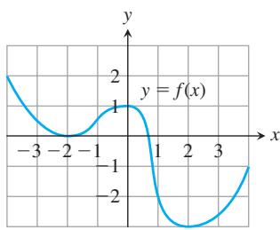
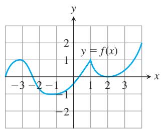
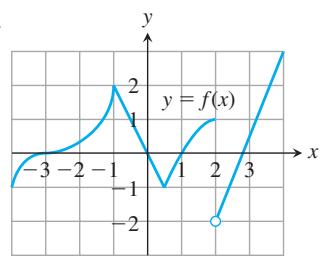
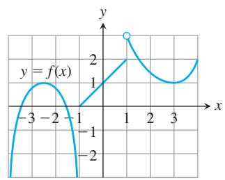
In Exercises 15–18:
a. Find the open intervals on which the function is increasing and those on which it is decreasing.
b. Identify the function’s local and absolute extreme values, if any, saying where they occur.
In Exercises 19–46:
a. Find the open intervals on which the function is increasing and those on which it is decreasing.
b. Identify the function’s local extreme values, if any, saying where they occur.
-
𝑔 ( 𝑡 ) = − 𝑡 2 − 3 𝑡 + 3 -
𝑔 ( 𝑡 ) = − 3 𝑡 2 + 9 𝑡 + 5 -
ℎ ( 𝑥 ) = − 𝑥 3 + 2 𝑥 2 -
ℎ ( 𝑥 ) = 2 𝑥 3 − 1 8 𝑥 -
𝑓 ( 𝜃 ) = 3 𝜃 2 − 4 𝜃 3 -
𝑓 ( 𝜃 ) = 6 𝜃 − 𝜃 3 -
𝑓 ( 𝑟 ) = 3 𝑟 3 + 1 6 𝑟 -
ℎ ( 𝑟 ) = ( 𝑟 + 7 ) 3 -
𝑓 ( 𝑥 ) = 𝑥 4 − 8 𝑥 2 + 1 6 -
𝐻 ( 𝑡 ) = 3 2 𝑡 4 − 𝑡 6
-
𝐾 ( 𝑡 ) = 1 5 𝑡 3 − 𝑡 5 -
𝑓 ( 𝑥 ) = 𝑥 − 6 √ 𝑥 − 1 -
𝑔 ( 𝑥 ) = 4 √ 𝑥 − 𝑥 2 + 3 -
𝑔 ( 𝑥 ) = 𝑥 √ 8 − 𝑥 2 -
𝑔 ( 𝑥 ) = 𝑥 2 √ 5 − 𝑥 -
𝑓 ( 𝑥 ) = 𝑥 2 − 3 𝑥 − 2 , 𝑥 ≠ 2 -
𝑓 ( 𝑥 ) = 𝑥 3 3 𝑥 2 + 1 -
𝑓 ( 𝑥 ) = 𝑥 1 / 3 ( 𝑥 + 8 ) -
𝑔 ( 𝑥 ) = 𝑥 2 / 3 ( 𝑥 + 5 ) -
ℎ ( 𝑥 ) = 𝑥 1 / 3 ( 𝑥 2 − 4 ) -
𝑘 ( 𝑥 ) = 𝑥 2 / 3 ( 𝑥 2 − 4 ) -
𝑓 ( 𝑥 ) = 𝑒 2 𝑥 + 𝑒 − 𝑥 -
𝑓 ( 𝑥 ) = 𝑒 √ 𝑥 -
𝑓 ( 𝑥 ) = 𝑥 l n 𝑥 -
𝑓 ( 𝑥 ) = 𝑥 2 l n 𝑥 -
𝑔 ( 𝑥 ) = 𝑥 ( l n 𝑥 ) 2 -
𝑔 ( 𝑥 ) = 𝑥 2 − 2 𝑥 − 4 l n 𝑥
In Exercises 47–58:
a. Identify the function’s local extreme values in the given domain, and say where they occur.
T b. Graph the function over the given domain. Which of the extreme values, if any, are absolute?
-
𝑓 ( 𝑥 ) = 2 𝑥 − 𝑥 2 , − ∞ < 𝑥 ≤ 2 -
𝑓 ( 𝑥 ) = ( 𝑥 + 1 ) 2 , − ∞ < 𝑥 ≤ 0 -
𝑔 ( 𝑥 ) = 𝑥 2 − 4 𝑥 + 4 , 1 ≤ 𝑥 < ∞ -
𝑔 ( 𝑥 ) = − 𝑥 2 − 6 𝑥 − 9 , − 4 ≤ 𝑥 < ∞ -
𝑓 ( 𝑡 ) = 1 2 𝑡 − 𝑡 3 , − 3 ≤ 𝑡 < ∞ -
𝑓 ( 𝑡 ) = 𝑡 3 − 3 𝑡 2 , − ∞ < 𝑡 ≤ 3 -
ℎ ( 𝑥 ) = 𝑥 3 3 − 2 𝑥 2 + 4 𝑥 , 0 ≤ 𝑥 < ∞ -
𝑘 ( 𝑥 ) = 𝑥 3 + 3 𝑥 2 + 3 𝑥 + 1 , − ∞ < 𝑥 ≤ 0 -
𝑓 ( 𝑥 ) = √ 2 5 − 𝑥 2 , − 5 ≤ 𝑥 ≤ 5 -
𝑓 ( 𝑥 ) = √ 𝑥 2 − 2 𝑥 − 3 , 3 ≤ 𝑥 < ∞ -
𝑔 ( 𝑥 ) = 𝑥 − 2 𝑥 2 − 1 , 0 ≤ 𝑥 < 1 -
𝑔 ( 𝑥 ) = 𝑥 2 4 − 𝑥 2 , − 2 < 𝑥 ≤ 1
In Exercises 59–66:
a. Find the local extrema of each function on the given interval, and say where they occur.
T b. Graph the function and its derivative together. Comment on the behavior of
-
𝑓 ( 𝑥 ) = s i n 2 𝑥 , 0 ≤ 𝑥 ≤ 𝜋 -
𝑓 ( 𝑥 ) = s i n 𝑥 − c o s 𝑥 , 0 ≤ 𝑥 ≤ 2 𝜋 -
𝑓 ( 𝑥 ) = √ 3 c o s 𝑥 + s i n 𝑥 , 0 ≤ 𝑥 ≤ 2 𝜋 -
𝑓 ( 𝑥 ) = − 2 𝑥 + t a n 𝑥 , − 𝜋 2 < 𝑥 < 𝜋 2 -
𝑓 ( 𝑥 ) = 𝑥 2 − 2 s i n 𝑥 2 , 0 ≤ 𝑥 ≤ 2 𝜋
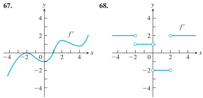
In Exercises 67 and 68, the graph of
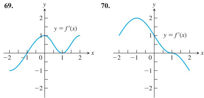
In Exercises 69 and 70, the graph of
a. Either use the graph to determine which intervals f is increasing on and which intervals f is decreasing on, or explain why this information cannot be determined from the graph.
b. Either use the graph to determine which intervals f is positive on and which intervals f is negative on, or explain why this information cannot be determined from the graph.
Theory and Examples
Show that the functions in Exercises 71 and 72 have local extreme values at the given values of
-
ℎ ( 𝜃 ) = 3 c o s 𝜃 2 , 0 ≤ 𝜃 ≤ 2 𝜋 , a t 𝜃 = 0 𝜃 = 2 𝜋 -
ℎ ( 𝜃 ) = 5 s i n 𝜃 2 , 0 ≤ 𝜃 ≤ 𝜋 , a t 𝜃 = 0 a n d 𝜃 = 𝜋 -
Sketch the graph of a differentiable function
𝑦 = 𝑓 ( 𝑥 ) 𝑓 ′ ( 1 ) = 0 𝑓 ′ ( 𝑥 ) > 0 𝑥 < 1 𝑓 ′ ( 𝑥 ) < 0 𝑥 > 1 𝑓 ′ ( 𝑥 ) < 0 𝑥 < 1 𝑓 ′ ( 𝑥 ) > 0 𝑥 > 1 𝑓 ′ ( 𝑥 ) > 0 𝑥 ≠ 1 𝑓 ′ ( 𝑥 ) < 0 𝑥 ≠ 1 -
Sketch the graph of a differentiable function
𝑦 = 𝑓 ( 𝑥 ) -
Sketch the graph of a continuous function
𝑦 = 𝑔 ( 𝑥 ) 𝑔 ( 2 ) = 2 , 0 < 𝑔 ′ < 1 𝑥 < 2 , 𝑔 ′ ( 𝑥 ) → 1 − 𝑥 → 2 − − 1 < 𝑔 ′ < 0 𝑥 > 2 𝑔 ′ ( 𝑥 ) → − 1 + 𝑥 → 2 + 𝑔 ( 2 ) = 2 , 𝑔 ′ < 0 𝑥 < 2 , 𝑔 ′ ( 𝑥 ) → − ∞ 𝑥 → 2 − 𝑔 ′ > 0 𝑥 > 2 𝑔 ′ ( 𝑥 ) → ∞ 𝑥 → 2 + -
Sketch the graph of a continuous function
𝑦 = ℎ ( 𝑥 ) ℎ ( 0 ) = 0 , − 2 ≤ ℎ ( 𝑥 ) ≤ 2 𝑥 , ℎ ′ ( 𝑥 ) → ∞ 𝑥 → 0 − ℎ ′ ( 𝑥 ) → ∞ 𝑥 → 0 + ℎ ( 0 ) = 0 , − 2 ≤ ℎ ( 𝑥 ) ≤ 0 𝑥 , ℎ ′ ( 𝑥 ) → ∞ 𝑥 → 0 − ℎ ′ ( 𝑥 ) → − ∞ 𝑥 → 0 + -
Discuss the extreme-value behavior of the function
𝑓 ( 𝑥 ) = 𝑥 s i n ( 1 / 𝑥 ) , 𝑥 ≠ 0 -
Find the open intervals on which the function
𝑓 ( 𝑥 ) = 𝑎 𝑥 2 + 𝑏 𝑥 + 𝑐 𝑎 ≠ 0
4.4 Concavity and Curve Sketching
-
Determine the values of constants a and b so that
𝑓 ( 𝑥 ) = 𝑎 𝑥 2 + 𝑏 𝑥 -
Determine the values of constants
𝑎 , 𝑏 , 𝑐 𝑑 𝑓 ( 𝑥 ) = 𝑎 𝑥 3 + 𝑏 𝑥 2 + 𝑐 𝑥 + 𝑑 -
Locate and identify the absolute extreme values of
a.
b.
- a. Prove that
𝑓 ( 𝑥 ) = 𝑥 − l n 𝑥
b. Using part (a), show that
-
Find the absolute maximum and the absolute minimum values of
𝑓 ( 𝑥 ) = 𝑒 𝑥 − 2 𝑥 [ 0 , 1 ] -
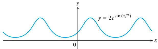
Where does the periodic function
𝑓 ( 𝑥 ) = 2 𝑒 s i n ( 𝑥 / 2 )
-
Find the absolute maximum value of
𝑓 ( 𝑥 ) = 𝑥 2 l n ( 1 / 𝑥 ) -
a. Prove that
𝑒 𝑥 ≥ 1 + 𝑥 𝑥 ≥ 0
b. Use the result in part (a) to show that
- Show that increasing functions and decreasing functions are one-to-one. That is, show that for any
𝑥 1 𝑥 2 𝐼 , 𝑥 2 ≠ 𝑥 1 𝑓 ( 𝑥 2 ) ≠ 𝑓 ( 𝑥 1 )
Use the results of Exercise 87 to show that the functions in Exercises 88–92 have inverses over their domains. Find a formula for
𝑓 ( 𝑥 ) = 𝑥 5 / 3
We have seen how the first derivative tells us where a function is increasing, where it is decreasing, and whether a local maximum or local minimum occurs at a critical point. In this section we see that the second derivative gives us information about how the graph of a differentiable function bends or turns. With this knowledge about the first and second derivatives, coupled with our previous understanding of symmetry and asymptotic behavior studied in Sections 1.1 and 2.5, we can now draw an accurate graph of a function. By organizing all of these ideas into a coherent procedure, we give a method for sketching graphs and revealing visually the key features of functions. Identifying and knowing the locations of these features is of major importance in mathematics and its applications to science and engineering, especially in the graphical analysis and interpretation of data. When the domain of a function is not a finite closed interval, sketching a graph helps to determine whether absolute maxima or absolute minima exist and, if they do exist, where they are located.
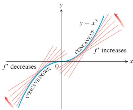
FIGURE 4.24 The graph of
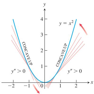
FIGURE 4.25 The graph of
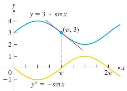
FIGURE 4.26 Using the sign of
Concavity
As you can see in Figure 4.24, the curve
DEFINITION The graph of a differentiable function
is 𝑦 = 𝑓 ( 𝑥 ) (a) concave up on an open interval I if
is increasing on I; 𝑓 ′ (b) concave down on an open interval I if
is decreasing on I. 𝑓 ′
A function whose graph is concave up is also often called convex.
If
The Second Derivative Test for Concavity
Let
-
If
𝑓 ″ > 0 𝐼 𝑓 𝐼 -
If
𝑓 ″ < 0
If
EXAMPLE 1
(a) The curve
(b) The curve
EXAMPLE 2 Determine the concavity of
Solution The first derivative of
Points of Inflection
The curve
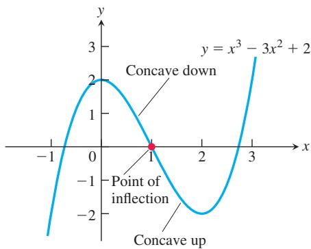
FIGURE 4.27 The concavity of the graph of f changes from concave down to concave up at the inflection point (Example 3).
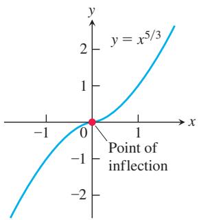
FIGURE 4.28 The graph of
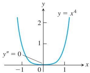
FIGURE 4.29 The graph of
DEFINITION A point
where the graph of a function has a tangent line and where the concavity changes is a point of inflection. ( 𝑐 , 𝑓 ( 𝑐 ) )
We observed that the second derivative of
At a point of inflection
EXAMPLE 3 Determine the concavity and find the inflection points of the function
Solution We start by computing the first and second derivatives.
To determine concavity, we look at the sign of the second derivative
The graph of f is shown in Figure 4.27. Notice that we did not need to know the shape of this graph ahead of time in order to determine its concavity.
The next example illustrates that a function can have a point of inflection where the first derivative exists but the second derivative fails to exist.
EXAMPLE 4 The graph of
fails to exist at x = 0. Nevertheless,
The following example shows that an inflection point need not occur even though both derivatives exist and
EXAMPLE 5 The curve
In the next example, a point of inflection occurs at a vertical tangent to the curve where neither the first nor the second derivative exists.
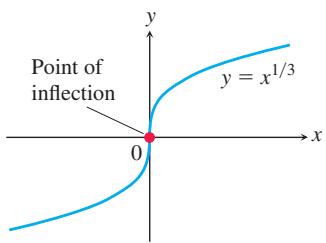
FIGURE 4.30 A point of inflection where
EXAMPLE 6 The graph of
However, both
Caution Example 4 in Section 4.1 (Figure 4.9) shows that the function
To study the motion of an object moving along a line as a function of time, we often are interested in knowing when the object’s acceleration, given by the second derivative, is positive or negative. The points of inflection on the graph of the object’s position function reveal where the acceleration changes sign.
EXAMPLE 7 A particle is moving along a horizontal coordinate line (positive to the right) with position function
Find the velocity and acceleration, and describe the motion of the particle.
Solution The velocity is
and the acceleration is
When the function
Notice that the first derivative
| Interval | 0 < t < 1 | 1 < t < 11/3 | 11/3 < t |
| Sign of | + | - | + |
| Behavior of s | increasing | decreasing | increasing |
| Particle motion | right | left | right |
The particle is moving to the right in the time intervals
The acceleration
| Interval | 0 < t < 7/3 | 7/3 < t |
| Sign of | - | + |
| Graph of s | concave down | concave up |
Under the influence of the leftward acceleration over the time interval
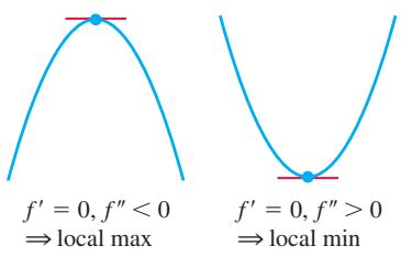
Second Derivative Test for Local Extrema
Instead of looking for sign changes in
THEOREM 5—Second Derivative Test for Local Extrema
Suppose
- If
𝑓 ′ ( 𝑐 ) = 0 𝑓 ″ ( 𝑐 ) < 0 𝑓 𝑥 = 𝑐 - If
𝑓 ′ ( 𝑐 ) = 0 𝑓 ″ ( 𝑐 ) > 0 𝑓 𝑥 = 𝑐 - If
𝑓 ′ ( 𝑐 ) = 0 𝑓 ″ ( 𝑐 ) = 0 𝑓
Proof Part (1). If
The proof of Part (2) is similar.
For Part (3), consider the three functions
This test requires us to know
Together
EXAMPLE 8 Sketch a graph of the function
using the following steps.
(a) Identify where the extrema of f occur.
(b) Find the intervals on which
(c) Find where the graph of
(d) Sketch the general shape of the graph for f.
(e) Plot some specific points, such as local maximum and minimum points, points of inflection, and intercepts. Then sketch the curve.
Solution The function
the first derivative is zero at x = 0 and x = 3. We use these critical points to define intervals where f is increasing or decreasing.
| Interval | |||
| Sign of | - | - | + |
| Behavior of | decreasing | decreasing | increasing |
(a) Using the First Derivative Test for local extrema and the table above, we see that there is no extremum at x = 0 and a local minimum at x = 3.
(b) Using the table above, we see that
(c)
| Interval | |||
| Sign of | + | - | + |
| Behavior of | concave up | concave down | concave up |
We see that the graph of
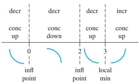
(d) Summarizing the information in the last two tables, we obtain the following.
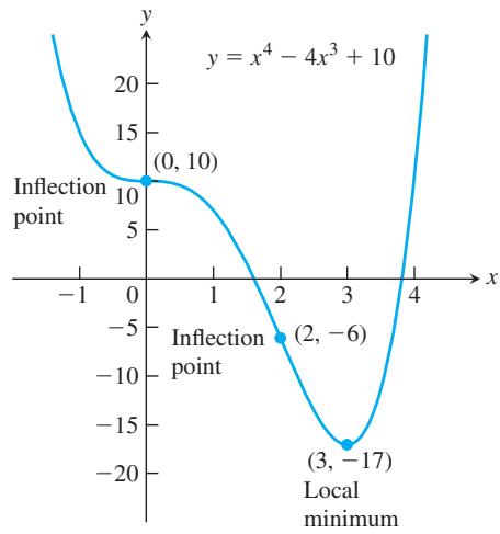
FIGURE 4.31 The graph of
| x < 0 | 0 < x < 2 | 2 < x < 3 | 3 < x |
| decreasing | decreasing | decreasing | increasing |
| concave up | concave down | concave up | concave up |
The general shape of the curve is shown in the accompanying figure.
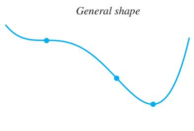
(e) Plot the curve’s intercepts (if possible) and the points where
The steps in Example 8 give a procedure for graphing the key features of a function. Asymptotes were defined and discussed in Section 2.5. We can find them for many classes of functions (including rational functions), and the methods in the next section give tools to help find them for even more general functions.
Procedure for Graphing
-
Identify the domain of f and any symmetries the curve may have.
-
Find the derivatives
𝑦 ′ 𝑦 ″ -
Find the critical points of
𝑓 -
Find where the curve is increasing and where it is decreasing.
-
Find the points of inflection, if any occur, and determine the concavity of the curve.
-
Identify any asymptotes that may exist.
-
Plot key points, such as the intercepts and the points found in Steps 3–5, and sketch the curve together with any asymptotes that exist.
EXAMPLE 9 Sketch the graph of
Solution
-
The domain of
𝑓 ( − ∞ , ∞ ) -
Find
𝑓 ′ 𝑓 ″
-
Behavior at critical points. The critical points occur only at
𝑥 = ± 1 𝑓 ′ ( 𝑥 ) = 0 𝑓 ′ 𝑓 𝑥 = − 1 𝑓 ″ ( − 1 ) = 1 > 0 𝑥 = 1 𝑓 ″ ( 1 ) = − 1 < 0 -
Increasing and decreasing. We see that on the interval
( − ∞ , − 1 ) 𝑓 ′ ( 𝑥 ) < 0 ( − 1 , 1 ) 𝑓 ′ ( 𝑥 ) > 0 ( 1 , ∞ ) 𝑓 ′ ( 𝑥 ) < 0 -
Inflection points. Notice that the denominator of the second derivative (Step 2) is always positive. The second derivative
𝑓 ″ 𝑥 = − √ 3 , 0 √ 3 ( − ∞ , − √ 3 ) ( − √ 3 , 0 ) ( 0 , √ 3 ) ( √ 3 , ∞ ) ( − ∞ , − √ 3 ) ( − √ 3 , 0 ) ( 0 , √ 3 ) ( √ 3 , ∞ )
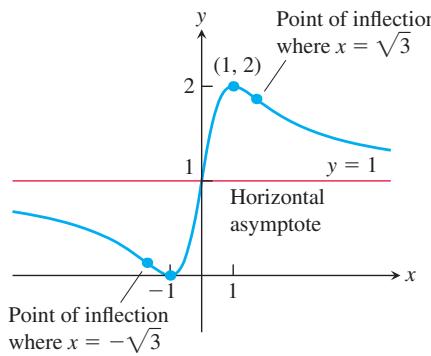
FIGURE 4.32 The graph of
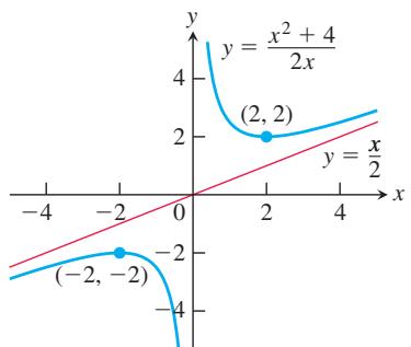
FIGURE 4.33 The graph of
- Asymptotes. Expanding the numerator of
𝑓 ( 𝑥 ) 𝑥 2
We see that
- The graph of
𝑓 𝑦 = 1 𝑥 → − ∞ 𝑦 = 1 𝑥 → ∞
EXAMPLE 10 Sketch the graph of
Solution
-
The domain of
𝑓 𝑥 𝑓 ( 𝑥 ) 𝑓 ( − 𝑥 ) = − 𝑓 ( 𝑥 ) 𝑓 𝑓 -
We calculate the derivatives of the function, but we first rewrite it in order to simplify our computations:
Function simplified for differentiation
Combine fractions to solve easily
Exists throughout the entire domain of
-
The critical points occur at
𝑥 = ± 2 𝑓 ′ ( 𝑥 ) = 0 𝑓 ″ ( − 2 ) < 0 𝑓 ″ ( 2 ) > 0 𝑥 = − 2 𝑓 ( − 2 ) = − 2 𝑥 = 2 𝑓 ( 2 ) = 2 -
On the interval
( − ∞ , − 2 ) 𝑓 ′ 𝑥 2 − 4 > 0 ( − 2 , 0 ) ( 0 , 2 ) ( 2 , ∞ ) -
There are no points of inflection because
𝑓 ″ ( 𝑥 ) < 0 𝑓 ″ ( 𝑥 ) > 0 𝑓 ″ ( − ∞ , 0 ) ( 0 , ∞ ) -
From the rewritten formula for
𝑓 ( 𝑥 )
so the
- The graph of
𝑓
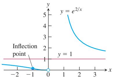
Solution The domain of
FIGURE 4.34 The graph of
FIGURE 4.35 The graph of the function in Example 12.
EXAMPLE 11 Sketch the graph of
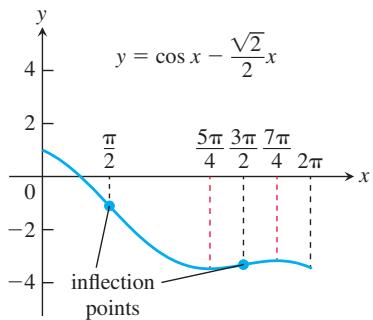
and
Both derivatives exist everywhere over the domain of
From Example 7, Section 2.5, we see that
EXAMPLE 12 Sketch the graph of
Solution The derivatives of
Both derivatives exist everywhere over the interval
Examining the second derivative, we find that
Finally, we evaluate
Graphical Behavior of Functions from Derivatives
As we saw in Examples 8–12, we can learn much about a twice-differentiable function
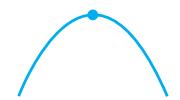
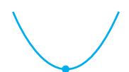
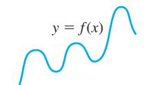 Differentiable ⇒ smooth, connected; graph may rise and fall Differentiable ⇒ smooth, connected; graph may rise and fall | 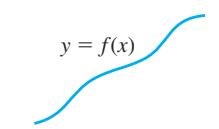 | 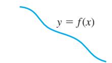 |
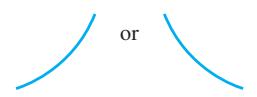 |  | 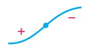 |
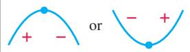 |  |  |
EXERCISES 4.4
Analyzing Functions from Graphs
Identify the inflection points and local maxima and minima of the functions graphed in Exercises 1–8. Identify the open intervals on which the functions are differentiable and the graphs are concave up and concave down.
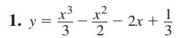
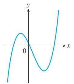
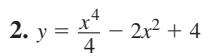
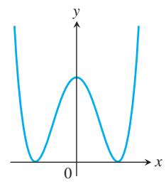
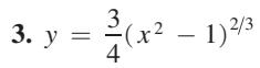
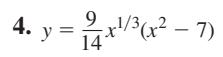
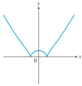
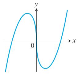

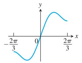

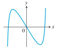
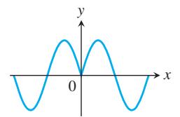

NOT TO SCALE
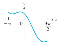
Graphing Functions
In Exercises 9–70, graph the function using appropriate methods from the graphing procedures presented just before Example 9, identifying the coordinates of any local extreme points and inflection points. Then find coordinates of absolute extreme points, if any.
-
𝑦 = 6 − 2 𝑥 − 𝑥 2 -
𝑦 = 𝑥 3 − 3 𝑥 + 3 -
𝑦 = 𝑥 ( 6 − 2 𝑥 ) 2 -
𝑦 = − 2 𝑥 3 + 6 𝑥 2 − 3
-
𝑦 = ( 𝑥 − 2 ) 3 + 1 -
𝑦 = 1 − ( 𝑥 + 1 ) 3 -
𝑦 = 𝑥 4 − 2 𝑥 2 = 𝑥 2 ( 𝑥 2 − 2 ) -
𝑦 = − 𝑥 4 + 6 𝑥 2 − 4 = 𝑥 2 ( 6 − 𝑥 2 ) − 4 -
𝑦 = 4 𝑥 3 − 𝑥 4 = 𝑥 3 ( 4 − 𝑥 ) -
𝑦 = 𝑥 4 + 2 𝑥 3 = 𝑥 3 ( 𝑥 + 2 ) -
𝑦 = 𝑥 5 − 5 𝑥 4 = 𝑥 4 ( 𝑥 − 5 ) -
𝑦 = 𝑥 ( 𝑥 2 − 5 ) 4 -
𝑦 = 2 𝑥 2 + 𝑥 − 1 𝑥 2 − 1 -
𝑦 = 𝑥 2 − 4 9 𝑥 2 + 5 𝑥 − 1 4 -
𝑦 = 𝑥 4 + 1 𝑥 2 -
𝑦 = 𝑥 2 − 4 2 𝑥 -
𝑦 = 1 𝑥 2 − 1 -
𝑦 = 𝑥 2 𝑥 2 − 1 -
𝑦 = − 𝑥 2 − 2 𝑥 2 − 1 -
𝑦 = 𝑥 2 − 4 𝑥 2 − 2 -
𝑦 = 𝑥 2 𝑥 + 1 -
𝑦 = − 𝑥 2 − 4 𝑥 + 1 -
𝑦 = 𝑥 2 − 𝑥 + 1 𝑥 − 1 -
𝑦 = − 𝑥 2 − 𝑥 + 1 𝑥 − 1 -
𝑦 = 𝑥 3 − 3 𝑥 2 + 3 𝑥 − 1 𝑥 2 + 𝑥 − 2 -
𝑦 = 𝑥 3 + 𝑥 − 2 𝑥 − 𝑥 2 -
𝑦 = 𝑥 𝑥 2 − 1 -
𝑦 = 4 𝑥 𝑥 2 + 4 -
𝑦 = 8 𝑥 2 + 4 -
𝑦 = 𝑥 √ 𝑥 2 + 1 -
𝑦 = 𝑥 + s i n 𝑥 , 0 ≤ 𝑥 ≤ 2 𝜋 -
𝑦 = 𝑥 − s i n 𝑥 , 0 ≤ 𝑥 ≤ 2 𝜋 -
𝑦 = √ 3 𝑥 − 2 c o s 𝑥 , 0 ≤ 𝑥 ≤ 2 𝜋 -
𝑦 = 4 3 𝑥 − t a n 𝑥 , − 𝜋 2 < 𝑥 < 𝜋 2 -
𝑦 = s i n 𝑥 c o s 𝑥 , 0 ≤ 𝑥 ≤ 𝜋 -
𝑦 = c o s 𝑥 + √ 3 s i n 𝑥 , 0 ≤ 𝑥 ≤ 2 𝜋 -
𝑦 = 𝑥 1 / 5 -
𝑦 = 𝑥 2 / 5 -
𝑦 = 2 𝑥 − 3 𝑥 2 / 3 -
𝑦 = 5 𝑥 2 / 5 − 2 𝑥 -
𝑦 = 𝑥 2 / 3 ( 5 2 − 𝑥 ) -
𝑦 = 𝑥 2 / 3 ( 𝑥 − 5 ) -
𝑦 = 𝑥 √ 8 − 𝑥 2 -
𝑦 = ( 2 − 𝑥 2 ) 3 / 2 -
𝑦 = √ 1 6 − 𝑥 2 -
𝑦 = 𝑥 2 + 2 𝑥 -
𝑦 = 𝑥 2 − 3 𝑥 − 2 -
𝑦 = 3 √ 𝑥 3 + 1 -
𝑦 = 8 𝑥 𝑥 2 + 4 -
𝑦 = 5 𝑥 4 + 5 -
𝑦 = | 𝑥 2 − 1 | -
𝑦 = | 𝑥 2 − 2 𝑥 | -
𝑦 = √ | 𝑥 | = { √ − 𝑥 , 𝑥 < 0 √ 𝑥 , 𝑥 ≥ 0 -
𝑦 = √ | 𝑥 − 4 | -
𝑦 = 𝑥 9 − 𝑥 2 -
𝑦 = 𝑥 2 1 − 𝑥 -
𝑦 = l n ( 3 − 𝑥 2 ) -
𝑦 = ( l n 𝑥 ) 2 -
𝑦 = l n ( c o s 𝑥 ) -
𝑦 = 1 1 + 𝑒 − 𝑥 = 𝑒 𝑥 1 + 𝑒 𝑥
Sketching the General Shape, Knowing 𝑦 ′
Each of Exercises 71–92 gives the first derivative of a continuous function
-
𝑦 ′ = 2 + 𝑥 − 𝑥 2 -
𝑦 ′ = 𝑥 2 − 𝑥 − 6 -
𝑦 ′ = 𝑥 ( 𝑥 − 3 ) 2 -
𝑦 ′ = 𝑥 2 ( 2 − 𝑥 ) -
𝑦 ′ = 𝑥 ( 𝑥 2 − 1 2 ) -
𝑦 ′ = ( 𝑥 − 1 ) 2 ( 2 𝑥 + 3 ) -
𝑦 ′ = ( 8 𝑥 − 5 𝑥 2 ) ( 4 − 𝑥 ) 2 -
𝑦 ′ = ( 𝑥 2 − 2 𝑥 ) ( 𝑥 − 5 ) 2 -
𝑦 ′ = s e c 2 𝑥 , − 𝜋 2 < 𝑥 < 𝜋 2 -
𝑦 ′ = t a n 𝑥 , − 𝜋 2 < 𝑥 < 𝜋 2 -
𝑦 ′ = c o t 𝜃 2 , 0 < 𝜃 < 2 𝜋 -
𝑦 ′ = c s c 2 𝜃 2 , 0 < 𝜃 < 2 𝜋 -
𝑦 ′ = t a n 2 𝜃 − 1 , − 𝜋 2 < 𝜃 < 𝜋 2 -
𝑦 ′ = 1 − c o t 2 𝜃 , 0 < 𝜃 < 𝜋 -
𝑦 ′ = c o s 𝑡 , 0 ≤ 𝑡 ≤ 2 𝜋 -
𝑦 ′ = s i n 𝑡 , 0 ≤ 𝑡 ≤ 2 𝜋 -
𝑦 ′ = ( 𝑥 + 1 ) − 2 / 3 -
𝑦 ′ = ( 𝑥 − 2 ) − 1 / 3 -
𝑦 ′ = 𝑥 − 2 / 3 ( 𝑥 − 1 ) -
𝑦 ′ = 𝑥 − 4 / 5 ( 𝑥 + 1 ) -
𝑦 ′ = 2 | 𝑥 | = { − 2 𝑥 , 𝑥 ≤ 0 2 𝑥 , 𝑥 > 0 -
𝑦 ′ = { − 𝑥 2 , 𝑥 ≤ 0 𝑥 2 , 𝑥 > 0
Sketching y from Graphs of
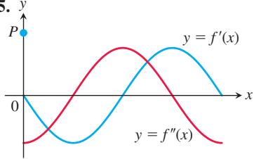
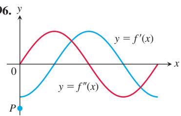
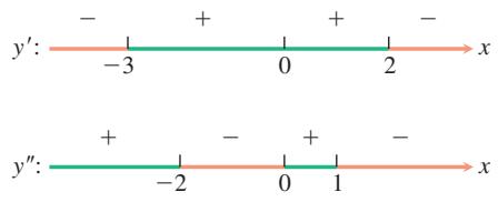
Each of Exercises 93–96 shows the graphs of the first and second derivatives of a function
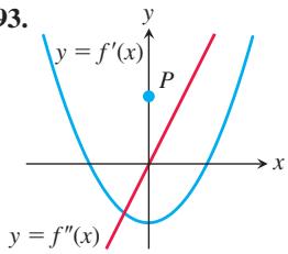
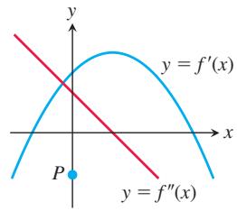
- y
- y
Theory and Examples
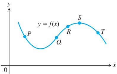
- The accompanying figure shows a portion of the graph of a twice-differentiable function
𝑦 = 𝑓 ( 𝑥 ) 𝑦 ′ 𝑦 ″
- Sketch a smooth connected curve
𝑦 = 𝑓 ( 𝑥 )
- Sketch the graph of a twice-differentiable function
𝑦 = 𝑓 ( 𝑥 )
| x | y | Derivatives |
| 2 | 1 | |
| 4 | 4 | |
| 6 | 7 | |
- Sketch the graph of a twice-differentiable function
𝑦 = 𝑓 ( 𝑥 ) ( − 2 , 2 ) , ( − 1 , 1 ) , ( 0 , 0 ) , ( 1 , 1 ) ( 2 , 2 )
- Sketch the graph of a twice-differentiable function
𝑦 = 𝑓 ( 𝑥 )
| x | y | Derivatives |
| -2 | -1 | |
| -1 | 0 | |
| 0 | 3 | |
| 1 | 2 | |
| 2 | 0 | |
- Sketch the graph of a twice-differentiable function
𝑦 = 𝑓 ( 𝑥 ) ( − 3 , − 2 ) ( − 2 , 0 ) ( 0 , 1 ) ( 1 , 2 ) ( 2 , 3 )
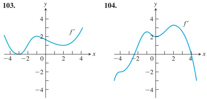
In Exercises 103 and 104, the graph of
In Exercises 105 and 106, the graph of
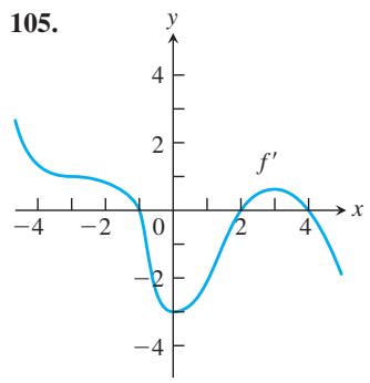
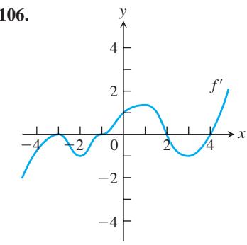
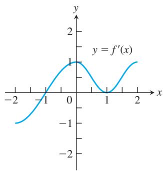
- A function
𝑓 ( 𝑥 ) ( − 2 , 2 ) 𝑦 = 𝑓 ′ ( 𝑥 )
- A function
𝑓 ( 𝑥 ) ( − 2 , 2 ) 𝑦 = 𝑓 ″ ( 𝑥 )
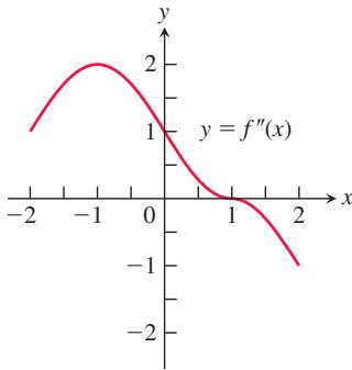
a. Either use the graph above to determine on which intervals the graph of f is concave up and on which intervals the graph of f is concave down and the inflection points of f, or explain why this information cannot be determined from the graph.
b. Either use the graph above to determine on which intervals
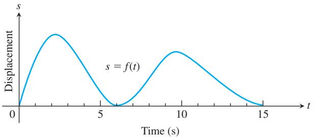
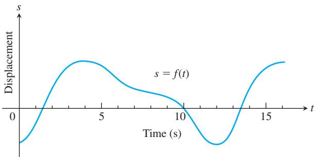
Motion Along a Line The graphs in Exercises 109 and 110 show the position
- Marginal cost The accompanying graph shows the hypothetical cost
𝑐 = 𝑓 ( 𝑥 ) 𝑥
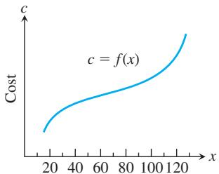
Thousands of units produced
- The accompanying graph shows the monthly revenue of the Widget Corporation for the past 12 years. During approximately what time intervals was the marginal revenue increasing? Decreasing?
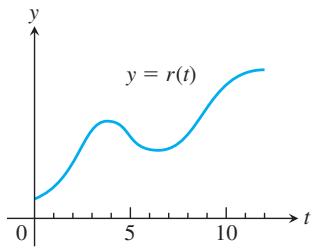
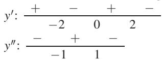
- Suppose the derivative of the function
𝑦 = 𝑓 ( 𝑥 )
At what points, if any, does the graph of f have a local minimum, local maximum, or point of inflection? (Hint: Draw the sign pattern for
- Suppose the derivative of the function
𝑦 = 𝑓 ( 𝑥 )
At what points, if any, does the graph of
-
For
𝑥 > 0 𝑦 = 𝑓 ( 𝑥 ) 𝑓 ( 1 ) = 0 𝑓 ′ ( 𝑥 ) = 1 / 𝑥 -
Can anything be said about the graph of a function
𝑦 = 𝑓 ( 𝑥 ) -
If
𝑏 , 𝑐 𝑑 𝑏 𝑦 = 𝑥 3 + 𝑏 𝑥 2 + 𝑐 𝑥 + 𝑑 𝑥 = 1 -
Parabolas
a. Find the coordinates of the vertex of the parabola
b. When is the parabola concave up? Concave down? Give reasons for your answers.
-
Quadratic curves What can you say about the inflection points of a quadratic curve
𝑦 = 𝑎 𝑥 2 + 𝑏 𝑥 + 𝑐 , 𝑎 ≠ 0 -
Cubic curves What can you say about the inflection points of a cubic curve
𝑦 = 𝑎 𝑥 3 + 𝑏 𝑥 2 + 𝑐 𝑥 + 𝑑 , 𝑎 ≠ 0 -
Suppose that the second derivative of the function
𝑦 = 𝑓 ( 𝑥 )
For what x-values does the graph of f have an inflection point?
- Suppose that the second derivative of the function
𝑦 = 𝑓 ( 𝑥 )
For what x-values does the graph of f have an inflection point?
-
Find the values of constants
𝑎 , 𝑏 𝑐 𝑦 = 𝑎 𝑥 3 + 𝑏 𝑥 2 + 𝑐 𝑥 𝑥 = 3 𝑥 = − 1 -
Find the values of constants
𝑎 , 𝑏 𝑐 𝑦 = ( 𝑥 2 + 𝑎 ) / ( 𝑏 𝑥 + 𝑐 ) 𝑥 = 3 ( − 1 , − 2 )
COMPUTER EXPLORATIONS
In Exercises 125–128, find the inflection points (if any) on the graph of the function and the coordinates of the points on the graph where the function has a local maximum or local minimum value. Then graph the function in a region large enough to show all these points simultaneously. Add to your picture the graphs of the function’s first and second derivatives. How are the values at which these graphs intersect the x-axis related to the graph of the function? In what other ways are the graphs of the derivatives related to the graph of the function?
-
𝑦 = 𝑥 5 − 5 𝑥 4 − 2 4 0 -
𝑦 = 𝑥 3 − 1 2 𝑥 2 -
𝑦 = 4 5 𝑥 5 + 1 6 𝑥 2 − 2 5 -
𝑦 = 𝑥 4 4 − 𝑥 3 3 − 4 𝑥 2 + 1 2 𝑥 + 2 0 -
Graph
𝑓 ( 𝑥 ) = 2 𝑥 4 − 4 𝑥 2 + 1 𝑓 ′ 𝑓 ″ -
Graph
𝑓 ( 𝑥 ) = 𝑥 c o s 𝑥 0 ≤ 𝑥 ≤ 2 𝜋 𝑓 ″
4.5 Indeterminate Forms and L’Hôpital’s Rule
Consider the four limits
In each case both the numerator and the denominator approach zero as
involves an indeterminate form 0/0. The expression “0/0” has the form of a number, but it is not a meaningful quantity. Stating that both the numerator and the denominator approach zero does not provide sufficient information to obtain the limit of the ratio. We have to examine the behavior of the expression in more detail by performing algebraic manipulation or by applying methods that we will introduce in this section.
HISTORICAL BIOGRAPHY
(1667-1748)
Johann Bernoulli was born in Switzerland and attended the University of Basel. His doctoral dissertation was in mathematics despite its medical title, which was used to hide his mathematical work from his father who wanted Johann to become a doctor.
Johann Bernoulli
In the late 1600s, John Fernoulle discovered a rule for calculating limits of fractions whose numerators and denominators both approach zero. Today the rule is known as l’Hôpital’s rule.
To know more, visit the companion Website.
To know more, visit the companion Website.
Guillaume François Antoine de l’Hôpital (1661–1704)
Other forms exhibit behavior similar to Equation (1). For instance, if both the numerator and the denominator approach
John (Johann) Bernoulli discovered a rule for using derivatives to calculate limits of fractions whose numerators and denominators both approach zero or
Indeterminate Form 0/0
It is important to understand that the notation “0/0” is not intended to imply numerically dividing 0 by 0. Instead, the indeterminate form 0/0 refers to a limit of a ratio of two functions, each of which approaches zero. L’Hôpital’s rule can help us evaluate such limits.
THEOREM 6—L’Hôpital’s Rule Suppose that
assuming that the limit on the right side of this equation exists.
We give a proof of Theorem 6 at the end of this section. Theorem 6 also applies if
Caution
EXAMPLE 1 The following limits involve 0/0 indeterminate forms, so we apply l’Hôpital’s Rule. In some cases, it must be applied repeatedly.
To apply l’Hôpital’s Rule to
(a)
(b)
(c)
(d)
(e)
Here is a summary of the procedure we followed in Example 1.
Using L’Hôpital’s Rule To find
by l’Hôpital’s Rule, we continue to differentiate
EXAMPLE 2 Be careful to apply l’Hôpital’s Rule correctly:
It is tempting to try to apply l’Hôpital’s Rule again, which would result in
but this is not the correct limit. l’Hôpital’s Rule can be applied only to limits that give indeterminate forms, and
L’Hôpital’s Rule applies to one-sided limits as well.
EXAMPLE 3 In this example the one-sided limits are different.
Indeterminate Forms ∞ / ∞ , ∞ ⋅ 0 , ∞ − ∞
Recall that
Sometimes when we try to evaluate a limit as
More advanced treatments of calculus prove that l’Hôpital’s Rule applies to the indeterminate form
provided the limit on the right exists or approaches
EXAMPLE 4 Find the limits of these
(a)
Solution
(a) The numerator and denominator are discontinuous at
The right-hand limit is 1 also, with
Next we turn our attention to the indeterminate forms
EXAMPLE 5 Find the limits of these
(a)
(b)
Solution
(See Example 6b in Section 2.5 for an alternative method to solve this problem.)
EXAMPLE 6 Find the limit of this
Solution If
Similarly, if
Neither form reveals what happens in the limit. To find out, we first combine the fractions:
Then we apply l’Hôpital’s Rule to the result:
Indeterminate Powers
Limits that lead to the indeterminate forms
If
Here a may be either finite or infinite.
EXAMPLE 7 Apply l’Hôpital’s Rule to show that
Solution The limit leads to the indeterminate form
l’Hôpital’s Rule now applies to give
Therefore,
EXAMPLE 8 Find
Solution The limit leads to the indeterminate form
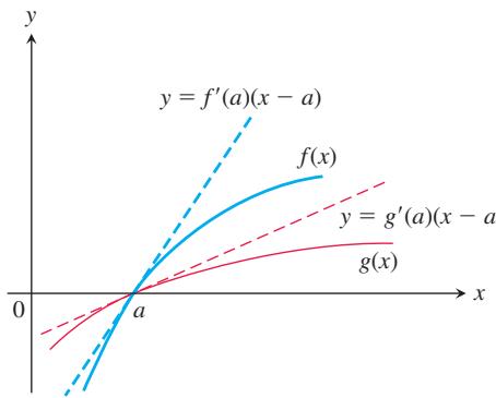
FIGURE 4.36 The two functions in l’Hôpital’s Rule, graphed with their linear approximations at
HISTORICAL BIOGRAPHY
Cauchy was born in Paris the year the French revolution began. He was the first to define fully the ideas of convergence and absolute convergence of infinite series. His classic works Cours d’analyse (Course on Analysis, 1821) and Résumé des leçons … sur le calcul infinitésimal (1823) were his greatest contributions to calculus.
To know more, visit the companion Website.
When
l’Hôpital’s Rule gives
Therefore,
Proof of L’Hôpital’s Rule
Before we prove l’Hôpital’s Rule, we consider a special case to provide some geometric insight for its reasonableness. Consider the two functions
where
as asserted by l’Hôpital’s Rule. We now proceed to a proof of the rule based on the more general assumptions stated in Theorem 6, which do not require that
The proof of l’Hôpital’s Rule is based on Cauchy’s Mean Value Theorem, an extension of the Mean Value Theorem that involves two functions instead of one. We prove Cauchy’s Theorem first and then show how it leads to l’Hôpital’s Rule.
THEOREM 7—Cauchy’s Mean Value Theorem
Suppose functions
Proof We apply the Mean Value Theorem of Section 4.2 twice. First we use it to show that
for some c between a and b, which cannot happen because
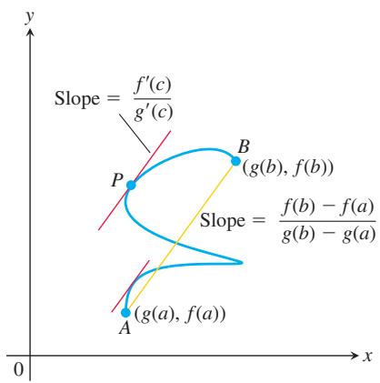
FIGURE 4.37 There is at least one point P on the curve C for which the slope of the tangent line to the curve at P is the same as the slope of the secant line joining the points
We next apply the Mean Value Theorem to the function
This function is continuous and differentiable where f and g are, and
so that
Cauchy’s Mean Value Theorem has a geometric interpretation for a general winding curve
the equation in Cauchy’s Mean Value Theorem says that the slope of the tangent line equals the slope of the secant line. This geometric interpretation is shown in Figure 4.37. Notice from the figure that it is possible for more than one point on the curve
Proof of l’Hôpital’s Rule Since
We first establish the limit equation for the case
Suppose that
But
As x approaches a, c approaches a because it always lies between a and x. Therefore,
which establishes l’Hôpital’s Rule for the case where
EXERCISES 4.5
Finding Limits in Two Ways
In Exercises 1–6, use l’Hôpital’s Rule to evaluate the limit. Then evaluate the limit using a method studied in Chapter 2.
-
l i m 𝑥 → − 2 𝑥 + 2 𝑥 2 − 4 -
l i m 𝑥 → 0 s i n 5 𝑥 𝑥 -
l i m 𝑥 → ∞ 5 𝑥 2 − 3 𝑥 7 𝑥 2 + 1 -
l i m 𝑥 → 1 𝑥 3 − 1 4 𝑥 3 − 𝑥 − 3 -
l i m 𝑥 → 0 1 − c o s 𝑥 𝑥 2 -
l i m 𝑥 → ∞ 2 𝑥 2 + 3 𝑥 𝑥 3 + 𝑥 + 1
Applying l’Hôpital’s Rule
Use l’Hôpital’s rule to find the limits in Exercises 7–52.
-
l i m 𝑥 → 2 𝑥 − 2 𝑥 2 − 4 -
l i m 𝑥 → − 5 𝑥 2 − 2 5 𝑥 + 5 -
l i m 𝑡 → − 3 𝑡 3 − 4 𝑡 + 1 5 𝑡 2 − 𝑡 − 1 2 -
l i m 𝑡 → − 1 3 𝑡 3 + 3 4 𝑡 3 − 𝑡 + 3 -
l i m 𝑥 → ∞ 5 𝑥 3 − 2 𝑥 7 𝑥 3 + 3 -
l i m 𝑥 → ∞ 𝑥 − 8 𝑥 2 1 2 𝑥 2 + 5 𝑥 -
l i m 𝑡 → 0 s i n 𝑡 2 𝑡 -
l i m 𝑡 → 0 s i n 5 𝑡 2 𝑡 -
l i m 𝑥 → 0 8 𝑥 2 c o s 𝑥 − 1 -
l i m 𝑥 → 0 s i n 𝑥 − 𝑥 𝑥 3 -
l i m 𝜃 → 𝜋 / 2 2 𝜃 − 𝜋 c o s ( 2 𝜋 − 𝜃 ) -
l i m 𝜃 → − 𝜋 / 3 3 𝜃 + 𝜋 s i n ( 𝜃 + ( 𝜋 / 3 ) ) -
l i m 𝜃 → 𝜋 / 6 s i n 𝜃 − 1 2 𝜃 − 𝜋 6 -
l i m 𝜃 → 𝜋 / 4 t a n 𝜃 − 1 𝜃 − 𝜋 4 -
l i m 𝜃 → 𝜋 / 2 1 − s i n 𝜃 1 + c o s 2 𝜃 -
l i m 𝑥 → 1 𝑥 − 1 l n 𝑥 − s i n 𝜋 𝑥 -
l i m 𝑥 → 0 𝑥 2 l n ( s e c 𝑥 ) -
l i m 𝑥 → 𝜋 / 2 l n ( c s c 𝑥 ) ( 𝑥 − ( 𝜋 / 2 ) ) 2 -
l i m 𝑡 → 0 𝑡 ( 1 − c o s 𝑡 ) 𝑡 − s i n 𝑡 -
l i m 𝑡 → 0 𝑡 s i n 𝑡 1 − c o s 𝑡 -
l i m 𝑥 → ( 𝜋 / 2 ) − ( 𝑥 − 𝜋 2 ) s e c 𝑥 -
l i m 𝑥 → ( 𝜋 / 2 ) − ( 𝜋 2 − 𝑥 ) t a n 𝑥 -
l i m 𝜃 → 0 3 s i n 𝜃 − 1 𝜃 -
l i m 𝜃 → 0 ( 1 / 2 ) 𝜃 − 1 𝜃 -
l i m 𝑥 → 0 𝑥 2 𝑥 2 𝑥 − 1 -
l i m 𝑥 → 0 3 𝑥 − 1 2 𝑥 − 1 -
l i m 𝑥 → ∞ l n ( 𝑥 + 1 ) l o g 2 𝑥 -
l i m 𝑥 → ∞ l o g 2 𝑥 l o g 3 ( 𝑥 + 3 ) -
l i m 𝑥 → 0 + l n ( 𝑥 2 + 2 𝑥 ) l n 𝑥 -
l i m 𝑥 → 0 + l n ( 𝑒 𝑥 − 1 ) l n 𝑥 -
l i m 𝑦 → 0 √ 5 𝑦 + 2 5 − 5 𝑦 -
l i m 𝑦 → 0 √ 𝑎 𝑦 + 𝑎 2 − 𝑎 𝑦 , 𝑎 > 0 -
l i m 𝑥 → ∞ ( l n 2 𝑥 − l n ( 𝑥 + 1 ) ) -
l i m 𝑥 → 0 + ( l n 𝑥 − l n s i n 𝑥 ) -
l i m 𝑥 → 0 + ( l n 𝑥 ) 2 l n ( s i n 𝑥 ) -
l i m 𝑥 → 0 + ( 3 𝑥 + 1 𝑥 − 1 s i n 𝑥 ) -
l i m 𝑥 → 1 + ( 1 𝑥 − 1 − 1 l n 𝑥 ) -
l i m 𝑥 → 0 + ( c s c 𝑥 − c o t 𝑥 + c o s 𝑥 ) -
l i m 𝜃 → 0 c o s 𝜃 − 1 𝑒 𝜃 − 𝜃 − 1 -
l i m ℎ → 0 𝑒 ℎ − ( 1 + ℎ ) ℎ 2 -
l i m 𝑡 → ∞ 𝑒 𝑡 + 𝑡 2 𝑒 𝑡 − 𝑡 -
l i m 𝑥 → ∞ 𝑥 2 𝑒 − 𝑥 -
l i m 𝑥 → 0 𝑥 − s i n 𝑥 𝑥 t a n 𝑥 -
l i m 𝑥 → 0 ( 𝑒 𝑥 − 1 ) 2 𝑥 s i n 𝑥 -
l i m 𝜃 → 0 𝜃 − s i n 𝜃 c o s 𝜃 t a n 𝜃 − 𝜃 -
l i m 𝑥 → 0 s i n 3 𝑥 − 3 𝑥 + 𝑥 2 s i n 𝑥 s i n 2 𝑥
Indeterminate Powers and Products
Find the limits in Exercises 53–68.
-
l i m 𝑥 → 1 + 𝑥 1 / ( 1 − 𝑥 ) -
l i m 𝑥 → 1 + 𝑥 1 / ( 𝑥 − 1 ) -
l i m 𝑥 → ∞ ( l n 𝑥 ) 1 / 𝑥 -
l i m 𝑥 → 𝑒 + ( l n 𝑥 ) 1 / ( 𝑥 − 𝑒 ) -
l i m 𝑥 → 0 + 𝑥 − 1 / l n 𝑥 -
l i m 𝑥 → ∞ 𝑥 1 / l n 𝑥 -
l i m 𝑥 → ∞ ( 1 + 2 𝑥 ) 1 / ( 2 l n 𝑥 ) -
l i m 𝑥 → 0 ( 𝑒 𝑥 + 𝑥 ) 1 / 𝑥 -
l i m 𝑥 → 0 + 𝑥 𝑥 -
l i m 𝑥 → 0 + ( 1 + 1 𝑥 ) 𝑥 -
l i m 𝑥 → ∞ ( 𝑥 + 2 𝑥 − 1 ) 𝑥 -
l i m 𝑥 → ∞ ( 𝑥 2 + 1 𝑥 + 2 ) 1 / 𝑥 -
l i m 𝑥 → 0 + 𝑥 2 l n 𝑥 -
l i m 𝑥 → 0 + 𝑥 ( l n 𝑥 ) 2 -
l i m 𝑥 → 0 + 𝑥 t a n ( 𝜋 2 − 𝑥 ) -
l i m 𝑥 → 0 + s i n 𝑥 ⋅ l n 𝑥
Theory and Applications
L’Hôpital’s Rule does not help with the limits in Exercises 69–76. Try it—you just keep on cycling. Find the limits some other way.
-
l i m 𝑥 → ∞ √ 9 𝑥 + 1 √ 𝑥 + 1 -
l i m 𝑥 → 0 + √ 𝑥 √ s i n 𝑥 -
l i m 𝑥 → ( 𝜋 / 2 ) − s e c 𝑥 t a n 𝑥 -
l i m 𝑥 → 0 + c o t 𝑥 c s c 𝑥 -
l i m 𝑥 → ∞ 2 𝑥 − 3 𝑥 3 𝑥 + 4 𝑥 -
l i m 𝑥 → − ∞ 2 𝑥 + 4 𝑥 5 𝑥 − 2 𝑥 -
l i m 𝑥 → ∞ 𝑒 𝑥 2 𝑥 𝑒 𝑥 -
l i m 𝑥 → 0 + 𝑥 𝑒 − 1 / 𝑥 -
Which one is correct, and which one is wrong? Give reasons for your answers. a.
l i m 𝑥 → 3 𝑥 − 3 𝑥 2 − 3 = l i m 𝑥 → 3 1 2 𝑥 = 1 6 l i m 𝑥 → 3 𝑥 − 3 𝑥 2 − 3 = 0 6 = 0 -
Which one is correct, and which one is wrong? Give reasons for your answers.
a.
- Only one of these calculations is correct. Which one? Why are the others wrong? Give reasons for your answers.
a.
b.
c.
d.
- Find all values of
𝑐
b.
continuous at
- For what values of
𝑎 𝑏

∞ − ∞
a. Estimate the value of
by graphing
b. Now confirm your estimate by finding the limit with l’Hôpital’s Rule. As the first step, multiply
- Find
l i m 𝑥 → ∞ ( √ 𝑥 2 + 1 − √ 𝑥 )

- 0/0 Form Estimate the value of
by graphing. Then confirm your estimate with l’Hôpital’s Rule. 86. This exercise explores the difference between
and
a. Use l’Hôpital’s Rule to show that
T b. Graph
together for
c. Confirm your estimate of
- Show that
- Given that
𝑥 > 0
a.
b.
c.
d. Show that
- Use limits to find horizontal asymptotes for each function.
a.
b.
- Find
𝑓 ′ ( 0 ) 𝑓 ( 𝑥 ) = { 𝑒 − 1 / 𝑥 2 , 𝑥 ≠ 0 0 , 𝑥 = 0 .

- T The continuous extension of
( s i n 𝑥 ) 𝑥 [ 0 , 𝜋 ]
a. Graph
b. Verify your conclusion in part (a) by finding
c. Returning to the graph, estimate the maximum value of
d. Sharpen your estimate in part (c) by graphing
- T The function
( s i n 𝑥 ) t a n 𝑥
a. Graph
b. Now graph
c. Continuing with the graphs in part (b), find
4.6 Applied Optimization
(a)
(b)
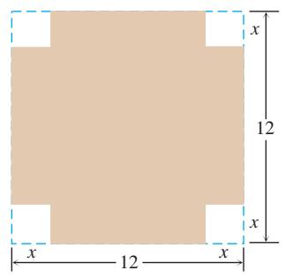
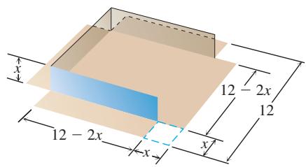
FIGURE 4.38 An open box made by cutting the corners from a square sheet of tin. What size corners maximize the box’s volume (Example 1)?
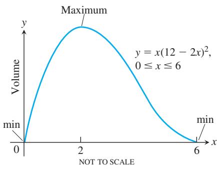
FIGURE 4.39 The volume of the box in Figure 4.38 graphed as a function of x.
What are the dimensions of a rectangle with fixed perimeter having maximum area? What are the dimensions for the least expensive cylindrical can of a given volume? How many items should be produced for the most profitable production run? Each of these questions asks for the best, or optimal, value of a given function. In this section we use derivatives to solve a variety of optimization problems in mathematics, physics, economics, and business.
Solving Applied Optimization Problems
-
Read the problem. Read the problem until you understand it. What is given? What is the unknown quantity to be optimized (maximized or minimized)?
-
Introduce variables. List every relevant relation in the problem as an equation. In most problems it is helpful to draw a picture.
-
Write an equation for the unknown quantity. Express the quantity to be optimized as a function of a single variable. This may require considerable manipulation.
-
Test the critical points and endpoints in the domain of the function found in the previous step. Use what you know about the shape of the function’s graph. Use the first and second derivatives to identify and classify the function’s critical points.
EXAMPLE 1 An open-top box is to be made by cutting small congruent squares from the corners of a 12-cm-by-12-cm sheet of tin and bending up the sides. How large should the squares cut from the corners be to make the box hold as much as possible?
Solution We start with a picture (Figure 4.38). In the figure, the corner squares are x cm on a side. The volume of the box is a function of this variable:
Since the sides of the sheet of tin are only 12 cm long,
A graph of V (Figure 4.39) suggests a minimum value of 0 at x = 0 and x = 6 and a maximum near x = 2. To learn more, we examine the first derivative of V with respect to x:
Of the two zeros,
Critical-point value:
Endpoint values:
The maximum volume is
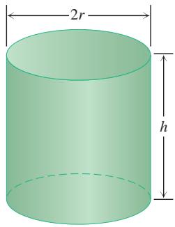
FIGURE 4.40 Example 2 shows that this one-liter can uses the least material when h = 2r.
EXAMPLE 2 You have been asked to design a one-liter can shaped like a right circular cylinder (Figure 4.40). What dimensions will use the least material?
Solution Volume of can: If r and h are measured in centimeters, then the volume of the can in cubic centimeters is
Surface area of can:
How can we interpret the phrase “least material”? For a first approximation we can ignore the thickness of the material and the waste in manufacturing. Then we ask for dimensions r and h that make the total surface area as small as possible, while satisfying the constraint
To express the surface area as a function of one variable, we solve for one of the variables in
Thus,
Our goal is to find a value of
Since A is differentiable on r > 0, an interval with no endpoints, it can have a minimum value only where its first derivative is zero.
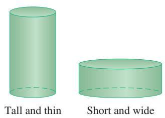
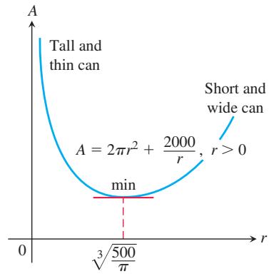
FIGURE 4.41 The graph of
What happens at
The second derivative
is positive throughout the domain of
The corresponding value of h (after a little algebra) is
The one-liter can that uses the least material has height equal to twice the radius, here with
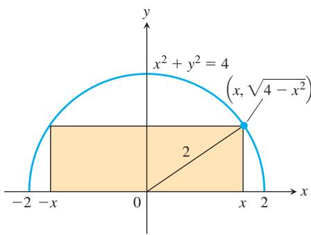
FIGURE 4.42 The rectangle inscribed in the semicircle in Example 3.
Examples from Mathematics and Physics
EXAMPLE 3 A rectangle is to be inscribed in a semicircle of radius 2. What is the largest area the rectangle can have, and what are its dimensions?
Solution Let
Notice that the values of
Our goal is to find the absolute maximum value of the function
on the domain [0, 2].
The derivative
is not defined when x = 2 and is equal to zero when
Of the two zeros,
The area has a maximum value of 4 when the rectangle is
HISTORICAL BIOGRAPHY Willebrord Snell van Royen (1580–1626)
Snell was born in Leiden, Holland. Snell developed an important result involving the measure of light refraction as it travels into different media. While he never published the result, Descartes did so ten years after Snell’s death, and today it is known as Snell’s law.
To know more, visit the companion Website.
EXAMPLE 4 The speed of light depends on the medium through which it travels, and is generally slower in denser media.
Fermat’s principle in optics states that light travels from one point to another along a path for which the time of travel is a minimum. Describe the path that a ray of light will follow in going from a point
Solution Since light traveling from A to B follows the quickest route, we look for a path that will minimize the travel time. We assume that A and B lie in the xy-plane and that the line separating the two media is the x-axis (Figure 4.43). We place A at coordinates
In a uniform medium, where the speed of light remains constant, “shortest time” means “shortest path,” and the ray of light will follow a straight line. Thus the path from A to B will consist of a line segment from A to a boundary point P, followed by another line segment from P to B. Distance traveled equals rate times time, so
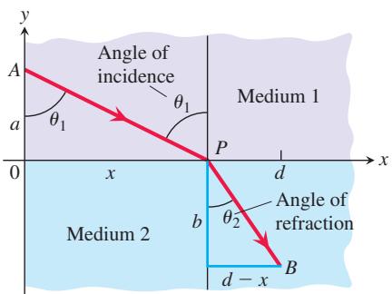
FIGURE 4.43 A light ray refracted (deflected from its path) as it passes from one medium to a denser medium (Example 4).
From Figure 4.43, the time required for light to travel from A to P is
FIGURE 4.44 The sign pattern of dt/dx in Example 4.
From
The time from A to B is the sum of these:
This equation expresses t as a differentiable function of x whose domain is
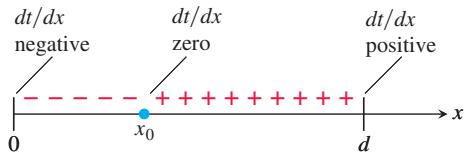
and observe that it is continuous. In terms of the angles
The function t has a negative derivative at x = 0 and a positive derivative at x = d. Since dt/dx is continuous over the interval
This equation is Snell’s Law or the Law of Refraction, and it is an important principle in the theory of optics. It describes the path the ray of light follows.
Examples from Economics
Suppose that
Although
If
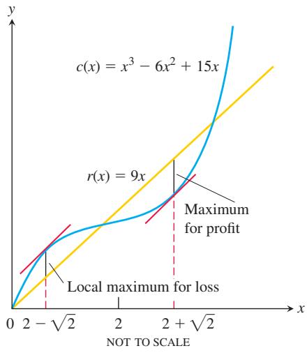
FIGURE 4.46 The cost and revenue curves for Example 5.
At a production level yielding maximum profit, marginal revenue equals marginal cost (Figure 4.45).
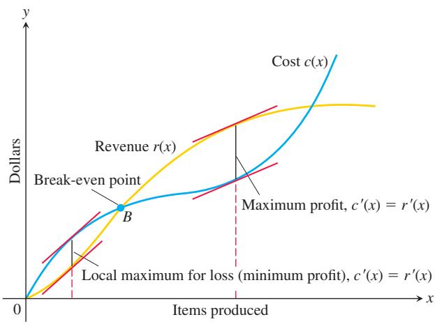
FIGURE 4.45 The graph of a typical cost function starts concave down and later turns concave up. It crosses the revenue curve at the break-even point B. To the left of B, the company operates at a loss. To the right, the company operates at a profit, with the maximum profit occurring where
EXAMPLE 5 Suppose that
Solution Notice that
The two solutions of the quadratic equation are
The possible production levels for maximum profit are
EXAMPLE 6 A cabinetmaker uses cherry wood to produce 5 desks each day. Each delivery of one container of wood is
Solution If she asks for a delivery every x days, then she must order 5x units to have enough material for that delivery cycle. The average amount in storage is approximately one-half of the delivery amount, or 5x/2. Thus, the cost of delivery and storage for each cycle is approximately
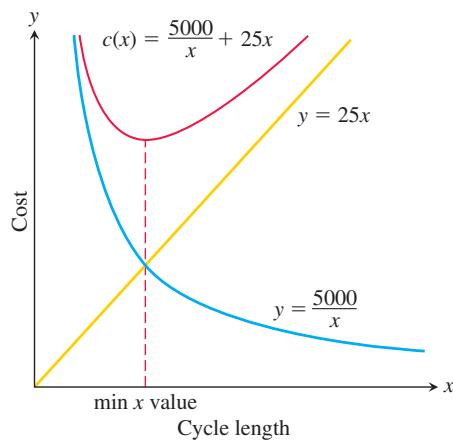
FIGURE 4.47 The average daily cost
We compute the average daily cost
As
We find the critical points by determining where the derivative is equal to zero:
Of the two critical points, only
We note that
The cabinetmaker should schedule a delivery of
EXERCISES 4.6
Mathematical Applications
Whenever you are maximizing or minimizing a function of a single variable, we urge you to graph it over the domain that is appropriate to the problem you are solving. The graph will provide insight before you calculate and will furnish a visual context for understanding your answer.
-
Minimizing perimeter What is the smallest perimeter possible for a rectangle whose area is
1 6 c m 2 -
Show that among all rectangles with an 8-m perimeter, the one with largest area is a square.
-
The figure shows a rectangle inscribed in an isosceles right triangle whose hypotenuse is 2 units long.
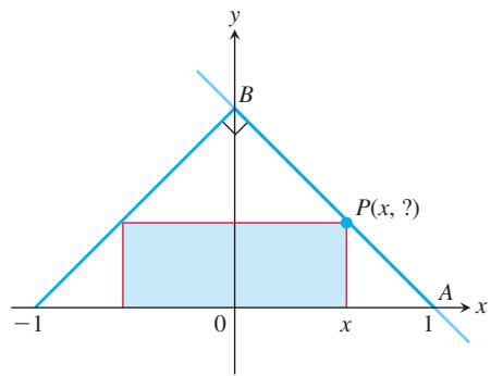
a. Express the y-coordinate of P in terms of x. (Hint: Write an equation for the line AB.)
b. Express the area of the rectangle in terms of x.
c. What is the largest area the rectangle can have, and what are its dimensions?
-
A rectangle has its base on the
𝑥 𝑦 = 1 2 − 𝑥 2 -
You are planning to make an open rectangular box from a 24-cm-by-45-cm piece of cardboard by cutting congruent squares from the corners and folding up the sides. What are the dimensions of the box of largest volume you can make this way, and what is its volume?
-
You are planning to close off a corner of the first quadrant with a line segment 20 units long running from
( 𝑎 , 0 ) ( 0 , 𝑏 ) 𝑎 = 𝑏 -
The best fencing plan A rectangular plot of farmland will be bounded on one side by a river and on the other three sides by a single-strand electric fence. With 800 m of wire at your disposal, what is the largest area you can enclose, and what are its dimensions?
-
The shortest fence A
2 1 6 𝑚 2
- Designing a tank Your iron works has contracted to design and build a
4 𝑚 3
a. What dimensions do you tell the shop to use?
b. Briefly describe how you took weight into account.
- Catching rainwater A 20 m
3
a. If the total cost is
what values of
b. Give a possible scenario for the cost function in part (a).
-
Designing a poster You are designing a rectangular poster to contain
3 1 2 . 5 𝑐 𝑚 2 -
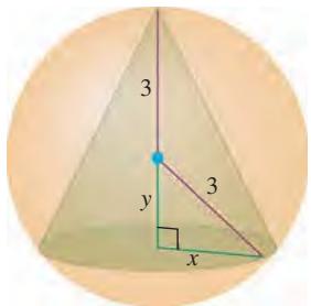
Find the volume of the largest right circular cone that can be inscribed in a sphere of radius 3.
-
Two sides of a triangle have lengths
𝑎 𝑏 𝜃 𝜃 𝐴 = ( 1 / 2 ) 𝑎 𝑏 s i n 𝜃 -
Designing a can What are the dimensions of the lightest open-top right circular cylindrical can that will hold a volume of
1 0 0 0 𝑐 𝑚 3 -
Designing a can You are designing a
1 0 0 0 𝑐 𝑚 3
rather than the
- Designing a box with a lid A piece of cardboard measures 30 cm by 45 cm. Two equal squares are removed from the corners of a 30-cm side as shown in the figure. Two equal rectangles are removed from the other corners so that the tabs can be folded to form a rectangular box with lid.
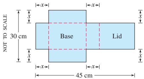
a. Write a formula
b. Find the domain of V for the problem situation, and graph V over this domain.
c. Use a graphical method to find the maximum volume and the value of x that gives it.
d. Confirm your result in part (c) analytically.
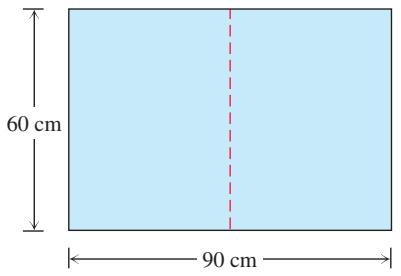
- Designing a suitcase A 60-cm-by-90-cm sheet of cardboard is folded in half to form a 60-cm-by-45-cm rectangle as shown in the accompanying figure. Then four congruent squares of side length x are cut from the corners of the folded rectangle. The sheet is unfolded, and the six tabs are folded up to form a box with sides and a lid.
a. Write a formula
b. Find the domain of V for the problem situation and graph V over this domain.
c. Use a graphical method to find the maximum volume and the value of x that gives it.
d. Confirm your result in part (c) analytically.
e. Find a value of x that yields a volume of
f. Write a paragraph describing the issues that arise in part (b).
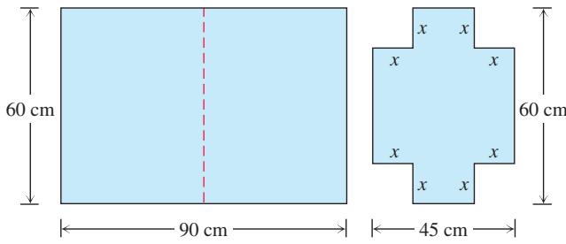
The sheet is then unfolded.
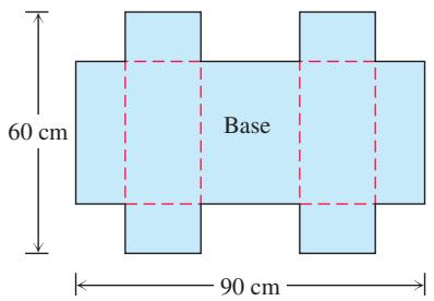
T 18. A rectangle is to be inscribed under the arch of the curve

-
Find the dimensions of a right circular cylinder of maximum volume that can be inscribed in a sphere of radius 10 cm. What is the maximum volume?
-
a. A certain Postal Service will accept a box for domestic shipment only if the sum of its length and girth (distance around) does not exceed 276 cm. What dimensions will give a box with a square end the largest possible volume?
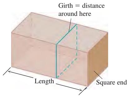
T b. Graph the volume of a 276-cm box (length plus girth equals 276 cm) as a function of its length, and compare what you see with your answer in part (a).
- (Continuation of Exercise 20)
a. Suppose that instead of having a box with square ends, you have a box with square sides so that its dimensions are
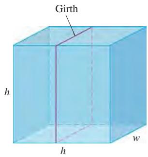
T b. Graph the volume as a function of h and compare what you see with your answer in part (a).
- A window is in the form of a rectangle surmounted by a semicircle. The rectangle is of clear glass, whereas the semicircle is of tinted glass that transmits only half as much light per unit area as clear glass does. The total perimeter is fixed. Find the proportions of the window that will admit the most light. Neglect the thickness of the frame.
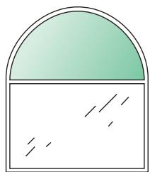
-
A silo (base not included) is to be constructed in the form of a cylinder surmounted by a hemisphere. The cost of construction per square unit of surface area is twice as great for the hemisphere as it is for the cylindrical sidewall. Determine the dimensions to be used if the volume is fixed and the cost of construction is to be kept to a minimum. Neglect the thickness of the silo and waste in construction.
-
The trough in the figure is to be made to the dimensions shown. Only the angle
𝜃 𝜃
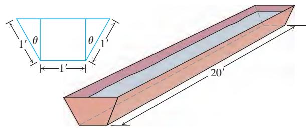
- Paper folding A rectangular sheet of 21.6-cm-by-28-cm paper is placed on a flat surface. One of the corners is placed on the opposite longer edge, as shown in the figure, and held there as the paper is smoothed flat. The problem is to make the length of the crease as small as possible. Call the length L. Try it with paper.
a. Show that
b. What value of
c. What is the minimum value of L?
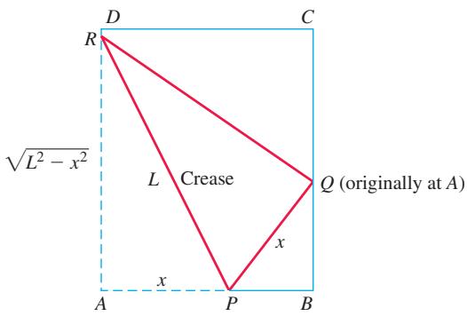
- Constructing cylinders Compare the answers to the following two construction problems.
a. A rectangular sheet of perimeter 36 cm and dimensions x cm by y cm is to be rolled into a cylinder as shown in part (a) of the figure. What values of x and y give the largest volume?
b. The same sheet is to be revolved about one of the sides of length
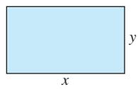
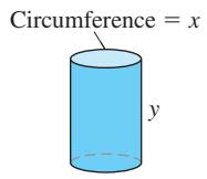
(a)
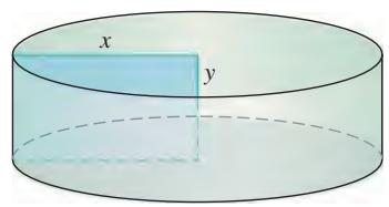
(b)
- Constructing cones A right triangle whose hypotenuse is
√ 3
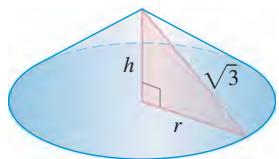
-
Find the point on the line
𝑥 𝑎 + 𝑦 𝑏 = 1 -
Find a positive number for which the sum of it and its reciprocal is the smallest (least) possible.
-
Find a positive number for which the sum of its reciprocal and four times its square is the smallest possible.
-
A wire b m long is cut into two pieces. One piece is bent into an equilateral triangle and the other is bent into a circle. If the sum of the areas enclosed by each part is a minimum, what is the length of each part?
-
Answer Exercise 31 if one piece is bent into a square and the other into a circle.
-
Suppose a weight D is to be held 5 m below a horizontal line AB by a wire in the shape of a Y. If the points A and B are 4 m apart, what is the minimum total length of wire that can be used?
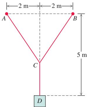
-
Suppose two different gauges of wire must be used to support the weight in Exercise 33: the vertical portion of the wire (the segment CD) costs
1 𝑝 𝑒 𝑟 𝑚 𝑒 𝑡 𝑒 𝑟 , 𝑤 ℎ 𝑖 𝑙 𝑒 𝑡 ℎ 𝑒 𝑟 𝑒 𝑚 𝑎 𝑖 𝑛 𝑖 𝑛 𝑔 𝑤 𝑖 𝑟 𝑒 ( 𝑡 ℎ 𝑒 𝑠 𝑒 𝑔 𝑚 𝑒 𝑛 𝑡 𝑠 𝐴 𝐶 𝑎 𝑛 𝑑 𝐶 𝐵 ) 𝑚 𝑢 𝑠 𝑡 𝑏 𝑒 𝑠 𝑡 𝑢 𝑟 𝑑 𝑖 𝑒 𝑟 𝑎 𝑛 𝑑 𝑐 𝑜 𝑠 𝑡 -
Determine the dimensions of the rectangle of largest area that can be inscribed in the right triangle shown in the accompanying figure.
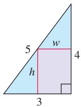
- Determine the dimensions of the rectangle of largest area that can be inscribed in a semicircle of radius 3. (See the accompanying figure.)
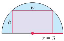
- What value of
𝑎 𝑓 ( 𝑥 ) = 𝑥 2 + ( 𝑎 / 𝑥 )
a. a local minimum at x = 2?
b. a point of inflection at
-
What values of
𝑎 𝑏 𝑓 ( 𝑥 ) = 𝑥 3 + 𝑎 𝑥 2 + 𝑏 𝑥 𝑥 = − 1 𝑥 = 3 𝑥 = 4 𝑥 = 1 -
A right circular cone is circumscribed by a sphere of radius 1. Determine the height h and radius r of the cone of maximum volume.
-
Determine the dimensions of the inscribed rectangle of maximum area.
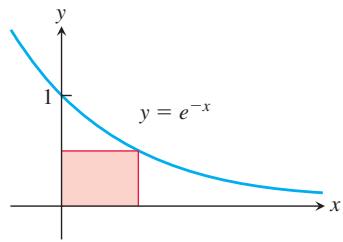
- Consider the accompanying graphs of
𝑦 = 2 𝑥 + 3 𝑦 = l n 𝑥
a. minimum vertical distance;
b. minimum horizontal distance between these graphs.
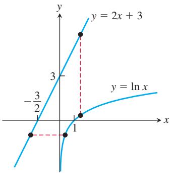
-
Find the point on the graph of
𝑦 = 2 0 𝑥 3 + 6 0 𝑥 − 3 𝑥 5 − 5 𝑥 4 -
Among all triangles in the first quadrant formed by the
𝑥 𝑦 𝑦 = 3 𝑥 − 𝑥 2
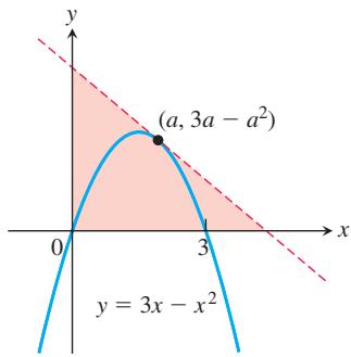
- A cone is formed from a circular piece of material of radius 1 meter by removing a section of angle
𝜃
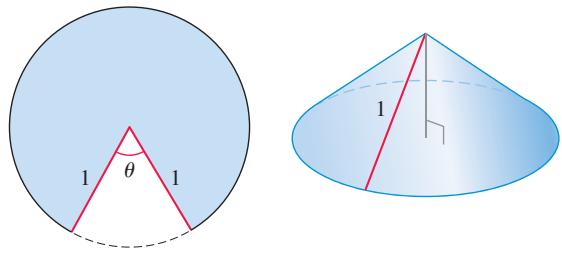
Physical Applications
- Vertical motion The height above ground of an object moving vertically is given by
with s in meters and t in seconds. Find
a. the object’s velocity when
b. its maximum height and when it occurs;
c. its velocity when s = 0.
-
Quickest route Jane is 2 km offshore in a boat and wishes to reach a coastal village 6 km down a straight shoreline from the point nearest the boat. She can row 2 km/h and can walk 5 km/h. Where should she land her boat to reach the village in the least amount of time?
-
Shortest beam The 2-m wall shown here stands 5 m from the building. Find the length of the shortest straight beam that will reach to the side of the building from the ground outside the wall.
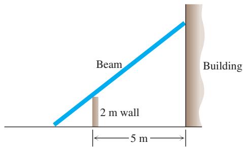
- Motion on a line The positions of two particles on the
𝑠 𝑠 1 = s i n 𝑡 𝑠 2 = s i n ( 𝑡 + 𝜋 / 3 ) 𝑠 1 𝑠 2 𝑡
a. At what time(s) in the interval
b. What is the farthest apart that the particles ever get?
c. When in the interval
-
The intensity of illumination at any point from a light source is proportional to the square of the reciprocal of the distance between the point and the light source. Two lights, one having an intensity eight times that of the other, are 6 m apart. How far from the stronger light is the total illumination least?
-
Projectile motion The range R of a projectile fired from the origin over horizontal ground is the distance from the origin to the point of impact. If the projectile is fired with an initial velocity
𝑣 0 𝛼
where g is the downward acceleration due to gravity. Find the angle
- Strength of a beam The strength S of a rectangular wooden beam is proportional to its width times the square of its depth. (See the accompanying figure.)
a. Find the dimensions of the strongest beam that can be cut from a 30-cm diameter cylindrical log.
b. Graph
c. On the same screen, graph
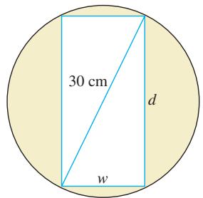
- Stiffness of a beam The stiffness S of a rectangular beam is proportional to its width times the cube of its depth.
a. Find the dimensions of the stiffest beam that can be cut from a 30-cm-diameter cylindrical log.
b. Graph
c. On the same screen, graph
- Frictionless cart A small frictionless cart, attached to the wall by a spring, is pulled 10 cm from its rest position and released at time t = 0 to roll back and forth for 4 s. Its position at time t is
𝑠 = 1 0 c o s 𝜋 𝑡
a. What is the cart’s maximum speed? When is the cart moving that fast? Where is it then? What is the magnitude of the acceleration then?
b. Where is the cart when the magnitude of the acceleration is greatest? What is the cart’s speed then?
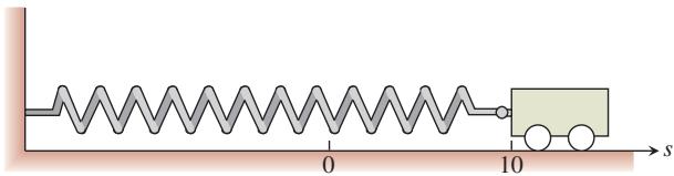
- Two masses hanging side by side from springs have positions
𝑠 1 = 2 s i n 𝑡 𝑠 2 = s i n 2 𝑡
a. At what times in the interval 0 < t do the masses pass each other? (Hint:
b. When in the interval
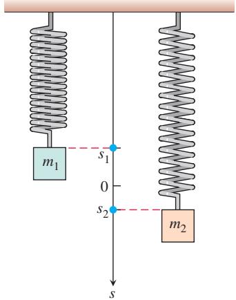
- Distance between two ships At noon, ship A was 12 nautical miles due north of ship B. Ship A was sailing south at 12 knots (nautical miles per hour; a nautical mile is 1852 m) and continued to do so all day. Ship B was sailing east at 8 knots and continued to do so all day.
a. Start counting time with t = 0 at noon and express the distance s between the ships as a function of t.
b. How rapidly was the distance between the ships changing at noon? One hour later?
c. The visibility that day was 5 nautical miles. Did the ships ever sight each other?
T d. Graph s and ds/dt together as functions of t for
e. The graph of
- Fermat’s principle in optics Light from a source
𝐴 𝐵
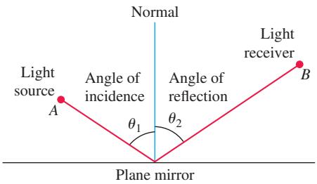
- Tin pest When metallic tin is kept below
1 3 . 2 ∘
A catalyst for a chemical reaction is a substance that controls the rate of reaction without undergoing any permanent change in itself. An autocatalytic reaction is one whose product is a catalyst for its own formation. Such a reaction may proceed slowly at first if the amount of catalyst present is small and slowly again at the end, when most of the original substance is used up. But in between, when both the substance and its catalyst product are abundant, the reaction proceeds at a faster pace.
In some cases, it is reasonable to assume that the rate
where
x = the amount of product,
a = the amount of substance at the beginning, and
At what value of x does the rate v have a maximum? What is the maximum value of v?
- Airplane landing path An airplane is flying at altitude H when it begins its descent to an airport runway that is at horizontal ground distance L from the airplane, as shown in the accompanying figure. Assume that the landing path of the airplane is the graph of a cubic polynomial function
𝑦 = 𝑎 𝑥 3 + 𝑏 𝑥 2 + 𝑐 𝑥 + 𝑑 𝑦 ( − 𝐿 ) = 𝐻 𝑦 ( 0 ) = 0
a. What is
b. What is
c. Use the values for
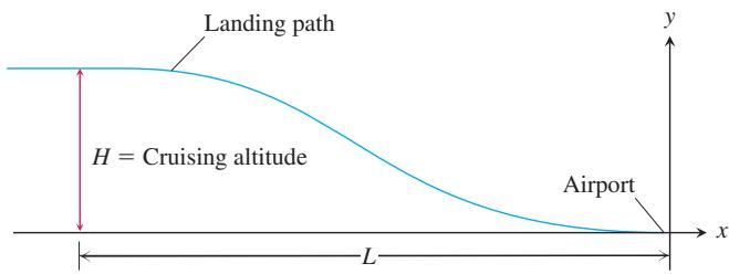
Business and Economics
- It costs you c dollars each to manufacture and distribute backpacks. If the backpacks sell at x dollars each, the number sold is given by
where
- You operate a tour service that offers the following rates:
$200 per person if 50 people (the minimum number to book the tour) go on the tour.
For each additional person, up to a maximum of 80 people total, the rate per person is reduced by $2.
It costs
- Wilson lot size formula One of the formulas for inventory management says that the average weekly cost of ordering, paying for, and holding merchandise is
where q is the quantity you order when things run low (shoes, radios, brooms, or whatever the item might be), k is the cost of placing an order (the same, no matter how often you order), c is the cost of one item (a constant), m is the number of items sold each week (a constant), and h is the weekly holding cost per item (a constant that takes into account things such as space, utilities, insurance, and security).
a. Your job, as the inventory manager for your store, is to find the quantity that will minimize
b. Shipping costs sometimes depend on order size. When they do, it is more realistic to replace k by
-
Production level Prove that the production level (if any) at which average cost is smallest is a level at which the average cost equals marginal cost.
-
Show that if
𝑟 ( 𝑥 ) = 6 𝑥 𝑐 ( 𝑥 ) = 𝑥 3 − 6 𝑥 2 + 1 5 𝑥 -
Production level Suppose that
𝑐 ( 𝑥 ) = 𝑥 3 − 2 0 𝑥 2 + 2 0 , 0 0 0 𝑥 -
You are to construct an open rectangular box with a square base and a volume of
6 𝑚 3 6 0 / 𝑚 2 4 0 / 𝑚 2 -
The 800-room Mega Motel chain is filled to capacity when the room charge is
5 0 𝑝 𝑒 𝑟 𝑛 𝑖 𝑔 ℎ 𝑡 . 𝐹 𝑜 𝑟 𝑒 𝑎 𝑐 ℎ
Biology
- Sensitivity to medicine (Continuation of Exercise 74, Section 3.3) Find the amount of medicine to which the body is most sensitive by finding the value of M that maximizes the derivative dR/dM, where
and
- How we cough
a. When we cough, the trachea (windpipe) contracts to increase the velocity of the air going out. This raises the questions of how much it should contract to maximize the velocity and whether it really contracts that much when we cough.
Under reasonable assumptions about the elasticity of the tracheal wall and about how the air near the wall is slowed by friction, the average flow velocity v can be modeled by the equation
where
Show that v is greatest when
T b. Take
Theory and Examples
- An inequality for positive integers Show that if
𝑎 , 𝑏 , 𝑐 𝑑
- The derivative dt/dx in Example 4
a. Show that
is an increasing function of
b. Show that
is a decreasing function of x.
c. Show that
is an increasing function of x.
- Let
𝑓 ( 𝑥 ) 𝑔 ( 𝑥 )
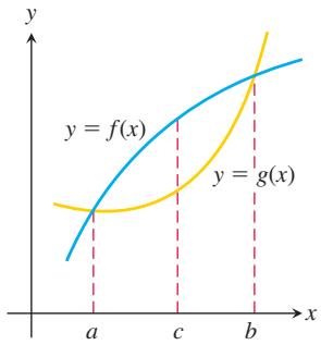
- You have been asked to determine whether the function
𝑓 ( 𝑥 ) = 3 + 4 c o s 𝑥 + c o s 2 𝑥
a. Explain why you need to consider values of x only in the interval
b. Is
- a. The function
𝑦 = c o t 𝑥 − √ 2 c s c 𝑥 0 < 𝑥 < 𝜋
T b. Graph the function and compare what you see with your answer in part (a).
- a. The function
𝑦 = t a n 𝑥 + 3 c o t 𝑥 0 < 𝑥 < 𝜋 / 2
T b. Graph the function and compare what you see with your answer in part (a).
- a. How close does the curve
𝑦 = √ 𝑥 ( 3 / 2 , 0 )
T b. Graph the distance function
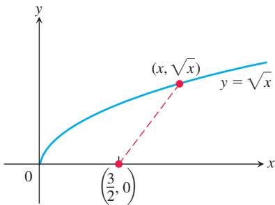
- a. How close does the semicircle
𝑦 = √ 1 6 − 𝑥 2 ( 1 , √ 3 )
T b. Graph the distance function and
4.7 Newton’s Method
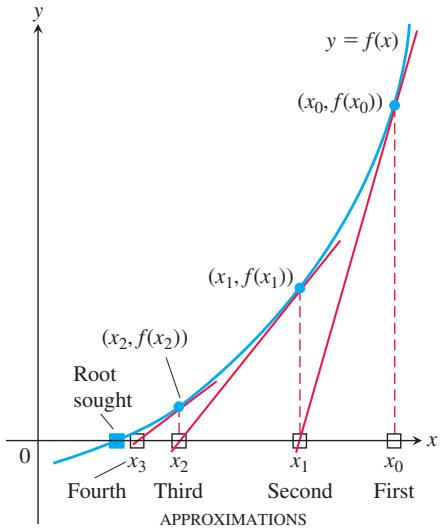
For thousands of years, one of the main goals of mathematics has been to find solutions to equations. For linear equations
FIGURE 4.48 Newton’s method starts with an initial guess
In this section we study a numerical method called Newton’s method or the Newton-Raphson method, which is a technique to approximate the solutions to an equation
Procedure for Newton’s Method
The goal of Newton’s method for estimating a solution of an equation
The initial estimate,
We can derive a formula for generating the successive approximations in the following way. Given the approximation
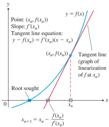
FIGURE 4.49 The geometry of the successive steps of Newton’s method. From
We can find where it crosses the x-axis by setting y = 0 (Figure 4.49):
This value of
Newton’s Method
-
Guess a first approximation to a solution of the equation
𝑓 ( 𝑥 ) = 0 𝑦 = 𝑓 ( 𝑥 ) -
Use the first approximation to get a second, the second to get a third, and so on, using the formula
Applying Newton’s Method
Applications of Newton’s method generally involve many numerical computations, making them well suited for computers or calculators. Nevertheless, even when the calculations are done by hand (which may be very tedious), they give a powerful way to find solutions of equations.
In our first example, we find decimal approximations to
EXAMPLE 1 Approximate the positive root of the equation
Solution With
The equation
enables us to go from each approximation to the next with just a few keystrokes. With the starting value
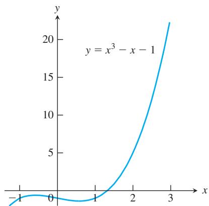
FIGURE 4.50 The graph of
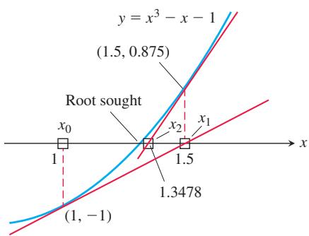
FIGURE 4.51 The first three x-values in Table 4.1 (four decimal places).
| Error | Number of correct digits | |
| -0.41421 | 1 | |
| 0.08579 | 1 | |
| 0.00246 | 3 | |
| 0.00001 | 5 |
Newton’s method is used by many software applications to calculate roots because it converges so fast (more about this later). If the arithmetic in the table in Example 1 had been carried to 13 decimal places instead of 5, then going one step further would have given
EXAMPLE 2 Find the x-coordinate of the point where the curve
Solution The curve crosses the line when
We apply Newton’s method to
At n = 5, we come to the result
TABLE 4.1 The Result of Applying Newton’s Method to
| n | ||||
| 0 | 1 | -1 | 2 | 1.5 |
| 1 | 1.5 | 0.875 | 5.75 | 1.3478 26087 |
| 2 | 1.3478 26087 | 0.1006 82173 | 4.4499 05482 | 1.3252 00399 |
| 3 | 1.3252 00399 | 0.0020 58362 | 4.2684 68292 | 1.3247 18174 |
| 4 | 1.3247 18174 | 0.0000 00924 | 4.2646 34722 | 1.3247 17957 |
| 5 | 1.3247 17957 | -1.8672E-13 | 4.2646 32999 | 1.3247 17957 |
In Figure 4.52 we have indicated that the process in Example 2 might have started at the point
Convergence of the Approximations
In Chapter 9 we define precisely the idea of convergence for the approximations
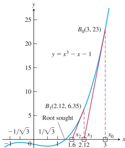
FIGURE 4.52 Any starting value
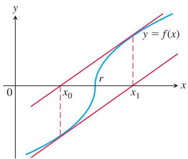
FIGURE 4.53 Newton’s method fails to converge. You go from
In practice, Newton’s method usually gives convergence with impressive speed, but this is not guaranteed. One way to test convergence is to begin by graphing the function to estimate a good starting value for
Newton’s method does not always converge. For instance, if
the graph will be like the one in Figure 4.53. If we begin with
If Newton’s method does converge, it converges to a root. Be careful, however. There are situations in which the method appears to converge but no root is there. Fortunately, such situations are rare.
When Newton’s method converges to a root, it may not be the root you have in mind. Figure 4.54 shows two ways this can happen.
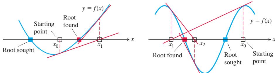
FIGURE 4.54 If you start too far away, Newton’s method may miss the root you want.
EXERCISES 4.7
Root Finding
-
Use Newton’s method to estimate the solutions of the equation
𝑥 2 + 𝑥 − 1 = 0 𝑥 0 = − 1 𝑥 0 = 1 𝑥 2 -
Use Newton’s method to estimate the one real solution of
𝑥 3 + 3 𝑥 + 1 = 0 𝑥 0 = 0 𝑥 2 -
Use Newton’s method to estimate the two zeros of the function
𝑓 ( 𝑥 ) = 𝑥 4 + 𝑥 − 3 𝑥 0 = − 1 𝑥 0 = 1 𝑥 2 -
Use Newton’s method to estimate the two zeros of the function
𝑓 ( 𝑥 ) = 2 𝑥 − 𝑥 2 + 1 𝑥 0 = 0 𝑥 0 = 2 𝑥 2 -
Use Newton’s method to find the positive fourth root of 2 by solving the equation
𝑥 4 − 2 = 0 𝑥 0 = 1 𝑥 2 -
Use Newton’s method to find the negative fourth root of 2 by solving the equation
𝑥 4 − 2 = 0 𝑥 0 = − 1 𝑥 2 -
T Use Newton’s method to find an approximate solution of
3 − 𝑥 = l n 𝑥 𝑥 0 = 2 𝑥 2 -
T Use Newton’s method to find an approximate solution of
𝑥 − 1 = a r c t a n 𝑥 𝑥 0 = 1 𝑥 2 -
T Use Newton’s method to find an approximate solution of
𝑥 𝑒 𝑥 = 1 𝑥 0 = 0 𝑥 2
Dependence on Initial Point
- Using the function shown in the figure, and, for each initial estimate
𝑥 0
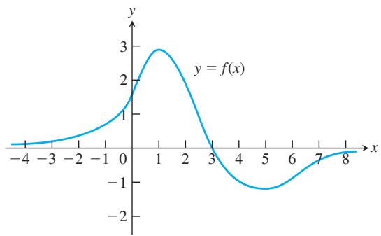
-
Guessing a root Suppose that your first guess is lucky, in the sense that
𝑥 0 𝑓 ( 𝑥 ) = 0 𝑓 ′ ( 𝑥 0 ) 𝑥 1 -
Estimating pi You plan to estimate
𝜋 / 2 c o s 𝑥 = 0
Theory and Examples
- Oscillation Show that if
ℎ > 0
leads to
-
Approximations that get worse and worse Apply Newton’s method to
𝑓 ( 𝑥 ) = 𝑥 1 / 3 𝑥 0 = 1 𝑥 1 , 𝑥 2 , 𝑥 3 𝑥 4 | 𝑥 𝑛 | | 𝑥 𝑛 | 𝑛 → ∞ -
Explain why the following four statements ask for the same information:
i) Find the roots of
ii) Find the
iii) Find the
iv) Find the values of
When solving Exercises 16–34, you may need to use appropriate technology (such as a calculator or a computer).
-
Locating a planet To calculate a planet’s space coordinates, we have to solve equations like
𝑥 = 1 + 0 . 5 s i n 𝑥 𝑓 ( 𝑥 ) = 𝑥 − 1 − 0 . 5 s i n 𝑥 𝑥 = 1 . 5 𝑥 0 = 1 . 5 𝑥 1 -
Intersecting curves The curve
𝑦 = t a n 𝑥 𝑦 = 2 𝑥 𝑥 = 0 𝑥 = 𝜋 / 2 -
Real solutions of a quartic Use Newton’s method to find the two real solutions of the equation
𝑥 4 − 2 𝑥 3 − 𝑥 2 − 2 𝑥 + 2 = 0 -
a. How many solutions does the equation
s i n 3 𝑥 = 0 . 9 9 − 𝑥 2
b. Use Newton’s method to find them.
- Intersection of curves
a. Does
b. Use Newton’s method to find where.
-
Find the four real zeros of the function
𝑓 ( 𝑥 ) = 2 𝑥 4 − 4 𝑥 2 + 1 -
Estimating pi Estimate
𝜋 t a n 𝑥 = 0 𝑥 0 = 3 -
Intersection of curves At what value(s) of x does
c o s 𝑥 = 2 𝑥 -
Intersection of curves At what value(s) of x does
c o s 𝑥 = − 𝑥 -
The graphs of
𝑦 = 𝑥 2 ( 𝑥 + 1 ) 𝑦 = 1 / 𝑥 ( 𝑥 > 0 ) 𝑥 = 𝑟 𝑟
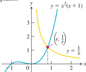
-
The graphs of
𝑦 = √ 𝑥 𝑦 = 3 − 𝑥 2 𝑥 = 𝑟 𝑟 -
Intersection of curves At what value(s) of
𝑥 𝑒 − 𝑥 2 = 𝑥 2 − 𝑥 + 1 -
Intersection of curves At what value(s) of
𝑥 l n ( 1 − 𝑥 2 ) = 𝑥 − 1 -
Use the Intermediate Value Theorem from Section 2.6 to show that
𝑓 ( 𝑥 ) = 𝑥 3 + 2 𝑥 − 4 -
Factoring a quartic Find the approximate values of
𝑟 1 𝑟 4
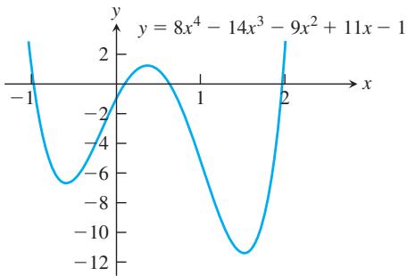
- Converging to different zeros Use Newton’s method to find the zeros of
𝑓 ( 𝑥 ) = 4 𝑥 4 − 4 𝑥 2
a.
b.
c.
d.
- The sonobuoy problem In submarine location problems, it is often necessary to find a submarine’s closest point of approach (CPA) to a sonobuoy (sound detector) in the water. Suppose that the submarine travels on the parabolic path
𝑦 = 𝑥 2 ( 2 , − 1 / 2 )
a. Show that the value of x that minimizes the distance between the submarine and the buoy is a solution of the equation
b. Solve the equation
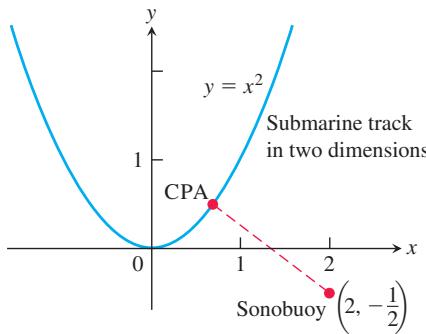
- Curves that are nearly flat at the root Some curves are so flat that, in practice, Newton’s method stops too far from the root to give a useful estimate. Try Newton’s method on
𝑓 ( 𝑥 ) = ( 𝑥 − 1 ) 4 0 𝑥 0 = 2
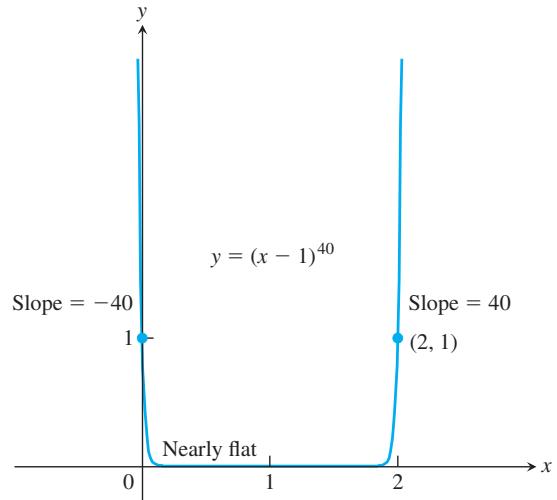
- The accompanying figure shows a circle of radius
𝑟 𝑠 𝑟 𝜃 0 < 𝜃 < 𝜋
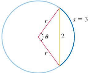
4.8 Antiderivatives
Many problems require that we recover a function from its derivative, or from its rate of change. For instance, the laws of physics tell us the acceleration of an object falling from an initial height, and we can use this to compute its velocity and its height at any time. More generally, starting with a function f, we want to find a function F whose derivative is f. If such a function F exists, it is called an antiderivative of f. Antiderivatives are the link connecting the two major elements of calculus: derivatives and definite integrals. Antiderivatives have an important connection to the theory of integrals that is developed in Chapter 5. For this reason the process of taking an antiderivative is also called “integration.”
Finding Antiderivatives
DEFINITION A function
is an antiderivative of 𝐹 on an interval 𝑓 if 𝐼 for all 𝐹 ′ ( 𝑥 ) = 𝑓 ( 𝑥 ) in 𝑥 . 𝐼
The process of recovering a function
EXAMPLE 1 Find an antiderivative for each of the following functions.
(a)
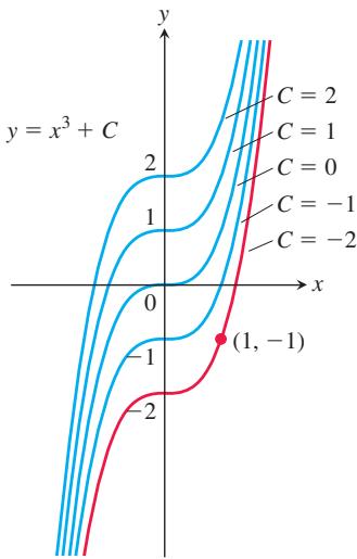
FIGURE 4.55 The curves
Solution We need to think backward here: What function do we know has a derivative equal to the given function?
Each answer can be checked by differentiating. The derivative of
The function
Corollary 2 of the Mean Value Theorem in Section 4.2 gives the answer: Any two antiderivatives of a function differ by a constant. So the functions
THEOREM 8 If F is an antiderivative of f on an interval I, then the most general antiderivative of f on I is
where C is an arbitrary constant.
Thus the most general antiderivative of f on I is a family of functions
EXAMPLE 2 Find an antiderivative of
Solution Since the derivative of
gives all the antiderivatives of
Since
is the antiderivative satisfying
By working backward from assorted differentiation rules, we can derive formulas and rules for antiderivatives. In each case there is an arbitrary constant C in the general expression representing all antiderivatives of a given function. Table 4.2 gives antiderivative formulas for a number of important functions.
The rules in Table 4.2 are easily verified by differentiating the general antiderivative formula to obtain the function to its left. For example, the derivative of
TABLE 4.2 Antiderivative formulas, k a nonzero constant
| Function | General antiderivative | Function | General antiderivative |
| 8. | |||
| 2. sin kx | 9. | ||
| 3. cos kx | 10. | ||
| 4. sec | 11. | ||
| 5. csc | 12. | ||
| 6. sec kx tan kx | 13. | ||
| 7. csc kx cot kx |
EXAMPLE 3 Find the general antiderivative of each of the following functions. (a)
Solution In each case, we can use one of the formulas listed in Table 4.2.
Other derivative rules also lead to corresponding antiderivative rules. We can add and subtract antiderivatives and multiply them by constants.
TABLE 4.3 Antiderivative linearity rules
| Function | General antiderivative | |
| 1. Constant Multiple Rule: | ||
| 2. Sum or Difference Rule: |
The formulas in Table 4.3 are easily proved by differentiating the antiderivatives and verifying that the result agrees with the original function.
EXAMPLE 4 Find the general antiderivative of
Solution We have that
is the general antiderivative formula for
Initial Value Problems and Differential Equations
Antiderivatives play several important roles in mathematics and its applications. Methods and techniques for finding them are a major part of calculus, and we take up that study in Chapter 8. Finding an antiderivative for a function
This is called a differential equation, since it is an equation involving an unknown function y that is being differentiated. To solve it, we need a function
This condition means the function
The most general antiderivative
Antiderivatives and Motion
We have seen that the derivative of the position function of an object gives its velocity, and the derivative of its velocity function gives its acceleration. If we know an object’s acceleration, then by finding an antiderivative we can recover the velocity, and from an antiderivative of the velocity we can recover its position function. This procedure was used as an application of Corollary 2 in Section 4.2. Now that we have a terminology and conceptual framework in terms of antiderivatives, we revisit the problem from the point of view of differential equations.
EXAMPLE 5 A hot-air balloon ascending at the rate of 3.6 m/s is at a height 24.5 m above the ground when a package is dropped. How long does it take the package to reach the ground?
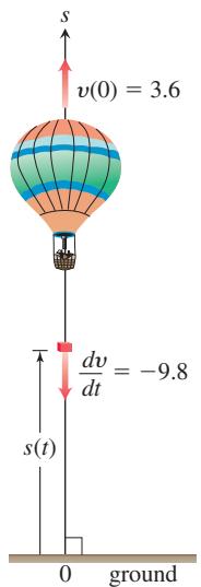
FIGURE 4.56 A package dropped from a rising hot-air balloon (Example 5).
Solution Let
This leads to the following initial value problem (Figure 4.56):
This is our mathematical model for the package’s motion. We solve the initial value problem to obtain the velocity of the package.
- Solve the differential equation: The general formula for an antiderivative of -9.8 is
Having found the general solution of the differential equation, we use the initial condition to find the particular solution that solves our problem.
2. Evaluate C:
The solution of the initial value problem is
Since velocity is the derivative of height, and the height of the package is
Differential equation:
We solve this initial value problem to find the height as a function of t.
- Solve the differential equation: Finding the general antiderivative of
− 9 . 8 𝑡 + 3 . 6
- Evaluate C:
The package’s height above ground at time
Use the solution: To find how long it takes the package to reach the ground, we set s equal to 0 and solve for t:
The package hits the ground about 2.63 s after it is dropped from the balloon. (The negative root has no physical meaning.)
Indefinite Integrals
A special symbol is used to denote the collection of all antiderivatives of a function f.
DEFINITION The collection of all antiderivatives of
is called the indefinite integral of 𝑓 with respect to 𝑓 ; it is denoted by 𝑥 ∫ 𝑓 ( 𝑥 ) 𝑑 𝑥 .
The symbol
After the integral sign in the notation we just defined, the integrand function is always followed by a differential to indicate the variable of integration. We will have more to say about why this is important in Chapter 5. Using this notation, we restate the solutions of Example 1, as follows:
This notation is related to the main application of antiderivatives, which will be explored in Chapter 5. Antiderivatives play a key role in computing limits of certain infinite sums, an unexpected and wonderfully useful role that is described in a central result of Chapter 5, the Fundamental Theorem of Calculus.
EXAMPLE 6 Evaluate
Solution If we recognize that
If we do not recognize the antiderivative right away, we can generate it term-by-term with the Sum, Difference, and Constant Multiple Rules:
This formula is more complicated than it needs to be. If we combine
and still gives all the possible antiderivatives there are. For this reason, we recommend that you go right to the final form even if you elect to integrate term-by-term. Write
Find the simplest antiderivative you can for each part, and add the arbitrary constant of integration at the end.
We conclude this section with a list of basic antidifferentiation formulas in Table 4.4, using the integral sign to indicate an antiderivative.
TABLE 4.4 Integration formulas
-
∫ 𝑥 𝑛 𝑑 𝑥 = 𝑥 𝑛 + 1 𝑛 + 1 + 𝐶 ( 𝑛 ≠ − 1 ) -
∫ s i n 𝑥 𝑑 𝑥 = − c o s 𝑥 + 𝐶 -
∫ c o s 𝑥 𝑑 𝑥 = s i n 𝑥 + 𝐶 -
∫ s e c 2 𝑥 𝑑 𝑥 = t a n 𝑥 + 𝐶 -
∫ c s c 2 𝑥 𝑑 𝑥 = − c o t 𝑥 + 𝐶 -
∫ s e c 𝑥 t a n 𝑥 𝑑 𝑥 = s e c 𝑥 + 𝐶 -
∫ 𝑒 𝑥 𝑑 𝑥 = 𝑒 𝑥 + 𝐶 -
∫ c s c 𝑥 c o t 𝑥 𝑑 𝑥 = − c s c 𝑥 + 𝐶 -
∫ 𝑑 𝑥 𝑥 = l n | 𝑥 | + 𝐶 ( 𝑥 ≠ 0 ) -
∫ 𝑑 𝑥 √ 1 − 𝑥 2 = a r c s i n 𝑥 + 𝐶 -
∫ 𝑑 𝑥 1 + 𝑥 2 = a r c t a n 𝑥 + 𝐶 -
∫ 𝑑 𝑥 𝑥 √ 𝑥 2 − 1 = a r c s e c 𝑥 + 𝐶 ( 𝑥 > 1 ) -
∫ 𝑎 𝑥 𝑑 𝑥 = 𝑎 𝑥 l n 𝑎 + 𝐶 ( 𝑎 > 0 , 𝑎 ≠ 1 )
EXERCISES 4.8
Finding Antiderivatives
In Exercises 1–24, find an antiderivative for each function. Do as many as you can mentally. Check your answers by differentiation.
- a. 2x
b.
c.
- a. 6x
b.
c.
- a.
− 3 𝑥 − 4
b.
c.
- a.
2 𝑥 − 3
b.
c.
- a.
1 𝑥 2
b.
- a.
− 2 𝑥 3
c.
- a.
3 2 √ 𝑥
b.
c.
- a.
4 3 3 √ 𝑥
b.
c.
- a.
2 3 𝑥 − 1 / 3
b.
c.
- a.
1 2 𝑥 − 1 / 2
c.
- a.
1 𝑥
b.
- a.
1 3 𝑥
c.
c.
-
a.
− 𝜋 s i n 𝜋 𝑥 3 s i n 𝑥 s i n 𝜋 𝑥 − 3 s i n 3 𝑥 -
a.
𝜋 c o s 𝜋 𝑥
b.
c.
- a.
s e c 2 𝑥
b.
c.
- a.
c s c 2 𝑥
b.
c.
- a.
c s c 𝑥 c o t 𝑥
c.
-
a.
s e c 𝑥 t a n 𝑥 4 s e c 3 𝑥 t a n 3 𝑥 s e c 𝜋 𝑥 2 t a n 𝜋 𝑥 2 -
a.
𝑒 3 𝑥
b.
c.
- a.
𝑒 − 2 𝑥
b.
c.
- a.
3 𝑥
b.
c.
- a.
𝑥 √ 3
c.
- a.
2 √ 1 − 𝑥 2
b.
c.
- a.
𝑥 − ( 1 2 ) 𝑥
c.
Finding Indefinite Integrals
In Exercises 25–70, find the most general antiderivative or indefinite integral. You may need to try a solution and then adjust your guess. Check your answers by differentiation.
-
∫ ( 𝑥 + 1 ) 𝑑 𝑥 -
∫ ( 5 − 6 𝑥 ) 𝑑 𝑥 -
∫ ( 3 𝑡 2 + 𝑡 2 ) 𝑑 𝑡 -
∫ ( 𝑡 2 2 + 4 𝑡 3 ) 𝑑 𝑡 -
∫ ( 2 𝑥 3 − 5 𝑥 + 7 ) 𝑑 𝑥 -
∫ ( 1 − 𝑥 2 − 3 𝑥 5 ) 𝑑 𝑥 -
∫ ( 1 𝑥 2 − 𝑥 2 − 1 3 ) 𝑑 𝑥 -
∫ ( 1 5 − 2 𝑥 3 + 2 𝑥 ) 𝑑 𝑥 -
∫ 𝑥 − 1 / 3 𝑑 𝑥 -
∫ 𝑥 − 5 / 4 𝑑 𝑥 -
∫ ( √ 𝑥 + 3 √ 𝑥 ) 𝑑 𝑥 -
∫ ( √ 𝑥 2 + 2 √ 𝑥 ) 𝑑 𝑥 -
∫ ( 8 𝑦 − 2 𝑦 1 / 4 ) 𝑑 𝑦 -
∫ ( 1 7 − 1 𝑦 5 / 4 ) 𝑑 𝑦 -
∫ 2 𝑥 ( 1 − 𝑥 − 3 ) 𝑑 𝑥 -
∫ 𝑥 − 3 ( 𝑥 + 1 ) 𝑑 𝑥 -
∫ 𝑡 √ 𝑡 + √ 𝑡 𝑡 2 𝑑 𝑡 -
∫ 4 + √ 𝑡 𝑡 3 𝑑 𝑡 -
∫ ( − 2 c o s 𝑡 ) 𝑑 𝑡 -
∫ ( − 5 s i n 𝑡 ) 𝑑 𝑡 -
∫ 7 s i n 𝜃 3 𝑑 𝜃 -
∫ 3 c o s 5 𝜃 𝑑 𝜃 -
∫ ( − 3 c s c 2 𝑥 ) 𝑑 𝑥 -
∫ ( − s e c 2 𝑥 3 ) 𝑑 𝑥 -
∫ c s c 𝜃 c o t 𝜃 2 𝑑 𝜃 -
∫ 2 5 s e c 𝜃 t a n 𝜃 𝑑 𝜃 -
∫ ( 𝑒 3 𝑥 + 5 𝑒 − 𝑥 ) 𝑑 𝑥 -
∫ ( 2 𝑒 𝑥 − 3 𝑒 − 2 𝑥 ) 𝑑 𝑥 -
∫ ( 𝑒 − 𝑥 + 4 𝑥 ) 𝑑 𝑥 -
∫ ( 1 . 3 ) 𝑥 𝑑 𝑥 -
∫ ( 4 s e c 𝑥 t a n 𝑥 − 2 s e c 2 𝑥 ) 𝑑 𝑥 -
∫ 1 2 ( c s c 2 𝑥 − c s c 𝑥 c o t 𝑥 ) 𝑑 𝑥 -
∫ ( s i n 2 𝑥 − c s c 2 𝑥 ) 𝑑 𝑥 -
∫ ( 2 c o s 2 𝑥 − 3 s i n 3 𝑥 ) 𝑑 𝑥 -
∫ 1 + c o s 4 𝑡 2 𝑑 𝑡 -
∫ 1 − c o s 6 𝑡 2 𝑑 𝑡 -
∫ ( 1 𝑥 − 5 𝑥 2 + 1 ) 𝑑 𝑥 -
∫ ( 2 √ 1 − 𝑦 2 − 1 𝑦 1 / 4 ) 𝑑 𝑦 -
∫ 3 𝑥 √ 3 𝑑 𝑥 -
∫ 𝑥 √ 2 − 1 𝑑 𝑥 -
∫ ( 1 + t a n 2 𝜃 ) 𝑑 𝜃 1 + t a n 2 𝜃 = s e c 2 𝜃 -
∫ ( 2 + t a n 2 𝜃 ) 𝑑 𝜃 -
∫ c o t 2 𝑥 𝑑 𝑥 -
∫ ( 1 − c o t 2 𝑥 ) 𝑑 𝑥 1 + c o t 2 𝑥 = c s c 2 𝑥 -
∫ c o s 𝜃 ( t a n 𝜃 + s e c 𝜃 ) 𝑑 𝜃 -
∫ c s c 𝜃 c s c 𝜃 − s i n 𝜃 𝑑 𝜃
Checking Antiderivative Formulas
Verify the formulas in Exercises 71–82 by differentiation.
∫ ( 7 𝑥 − 2 ) 3 𝑑 𝑥 = ( 7 𝑥 − 2 ) 4 2 8 + 𝐶
-
∫ 1 ( 𝑥 + 1 ) 2 𝑑 𝑥 = − 1 𝑥 + 1 + 𝐶 -
∫ 1 ( 𝑥 + 1 ) 2 𝑑 𝑥 = 𝑥 𝑥 + 1 + 𝐶 -
∫ 1 𝑥 + 1 𝑑 𝑥 = l n | 𝑥 + 1 | + 𝐶 , 𝑥 ≠ − 1 -
∫ 𝑥 𝑒 𝑥 𝑑 𝑥 = 𝑥 𝑒 𝑥 − 𝑒 𝑥 + 𝐶 -
∫ 𝑑 𝑥 𝑎 2 + 𝑥 2 = 1 𝑎 a r c t a n ( 𝑥 𝑎 ) + 𝐶 -
∫ 𝑑 𝑥 √ 𝑎 2 − 𝑥 2 = a r c s i n ( 𝑥 𝑎 ) + 𝐶 -
∫ a r c t a n 𝑥 𝑥 2 𝑑 𝑥 = l n 𝑥 − 1 2 l n ( 1 + 𝑥 2 ) − a r c t a n 𝑥 𝑥 + 𝐶 -
∫ ( a r c s i n 𝑥 ) 2 𝑑 𝑥 = 𝑥 ( a r c s i n 𝑥 ) 2 − 2 𝑥 + 2 √ 1 − 𝑥 2 a r c s i n 𝑥 + 𝐶 -
Right, or wrong? Say which for each formula and give a brief reason for each answer.
a.
c.
- Right, or wrong? Say which for each formula and give a brief reason for each answer.
c.
- Right, or wrong? Say which for each formula and give a brief reason for each answer.
a.
b.
c.
- Right, or wrong? Say which for each formula and give a brief reason for each answer.
a.
b.
c.
- Right, or wrong? Give a brief reason why.
Initial Value Problems
- Which of the following graphs shows the solution of the initial value problem
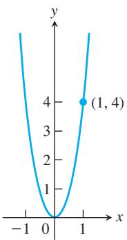
(a)
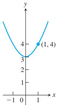
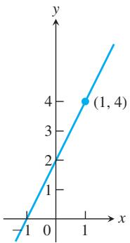
(b)
(c)
Give reasons for your answer.
- Which of the following graphs shows the solution of the initial value problem
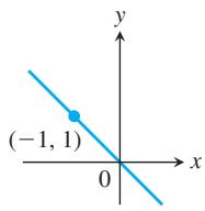
(a)
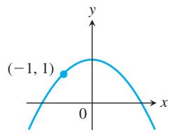
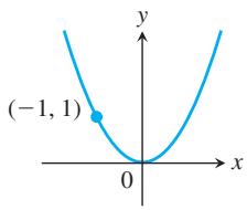
(b)
(c)
Give reasons for your answer.
Solve the initial value problems in Exercises 91–112.
-
𝑑 𝑦 𝑑 𝑥 = 2 𝑥 − 7 , 𝑦 ( 2 ) = 0 -
𝑑 𝑦 𝑑 𝑥 = 1 0 − 𝑥 , 𝑦 ( 0 ) = − 1 -
𝑑 𝑦 𝑑 𝑥 = 1 𝑥 2 + 𝑥 , 𝑥 > 0 ; 𝑦 ( 2 ) = 1 -
𝑑 𝑦 𝑑 𝑥 = 9 𝑥 2 − 4 𝑥 + 5 , 𝑦 ( − 1 ) = 0 -
𝑑 𝑦 𝑑 𝑥 = 3 𝑥 − 2 / 3 𝑦 ( − 1 ) = − 5 -
𝑑 𝑦 𝑑 𝑥 = 1 2 √ 𝑥 , 𝑦 ( 4 ) = 0 -
𝑑 𝑠 𝑑 𝑡 = 1 + c o s 𝑡 , 𝑠 ( 0 ) = 4 -
𝑑 𝑠 𝑑 𝑡 = c o s 𝑡 + s i n 𝑡 , 𝑠 ( 𝜋 ) = 1 -
𝑑 𝑟 𝑑 𝜃 = − 𝜋 s i n 𝜋 𝜃 , 𝑟 ( 0 ) = 0 -
𝑑 𝑟 𝑑 𝜃 = c o s 𝜋 𝜃 , 𝑟 ( 0 ) = 1 -
𝑑 𝑣 𝑑 𝑡 = 1 2 s e c 𝑡 t a n 𝑡 , 𝑣 ( 0 ) = 1 -
𝑑 𝜐 𝑑 𝑡 = 8 𝑡 + c s c 2 𝑡 , 𝜐 ( 𝜋 2 ) = − 7 -
𝑑 𝑣 𝑑 𝑡 = 3 𝑡 √ 𝑡 2 − 1 , 𝑡 > 1 , 𝑣 ( 2 ) = 0 -
𝑑 𝑣 𝑑 𝑡 = 8 1 + 𝑡 2 + s e c 2 𝑡 , 𝑣 ( 0 ) = 1 -
𝑑 2 𝑦 𝑑 𝑥 2 = 2 − 6 𝑥 ; 𝑦 ′ ( 0 ) = 4 , 𝑦 ( 0 ) = 1 -
𝑑 2 𝑦 𝑑 𝑥 2 = 0 ; 𝑦 ′ ( 0 ) = 2 , 𝑦 ( 0 ) = 0 -
𝑑 2 𝑟 𝑑 𝑡 2 = 2 𝑡 3 ; 𝑑 𝑟 𝑑 𝑡 ∣ 𝑡 = 1 = 1 , 𝑟 ( 1 ) = 1 -
𝑑 2 𝑠 𝑑 𝑡 2 = 3 𝑡 8 ; 𝑑 𝑠 𝑑 𝑡 ∣ 𝑡 = 4 = 3 , 𝑠 ( 4 ) = 4 -
𝑑 3 𝑦 𝑑 𝑥 3 = 6 ; 𝑦 ″ ( 0 ) = − 8 , 𝑦 ′ ( 0 ) = 0 , 𝑦 ( 0 ) = 5 -
𝑑 3 𝜃 𝑑 𝑡 3 = 0 ; 𝜃 ″ ( 0 ) = − 2 , 𝜃 ′ ( 0 ) = − 1 2 , 𝜃 ( 0 ) = √ 2 -
𝑦 ( 4 ) = − s i n 𝑡 + c o s 𝑡 ; 𝑦 ‴ ( 0 ) = 7 , 𝑦 ″ ( 0 ) = 𝑦 ′ ( 0 ) = − 1 , 𝑦 ( 0 ) = 0 -
𝑦 ( 4 ) = − c o s 𝑥 + 8 s i n 2 𝑥 ; 𝑦 ‴ ( 0 ) = 0 , 𝑦 ″ ( 0 ) = 𝑦 ′ ( 0 ) = 1 , 𝑦 ( 0 ) = 3 -
Find the curve
𝑦 = 𝑓 ( 𝑥 ) 3 √ 𝑥 -
a. Find a curve
𝑦 = 𝑓 ( 𝑥 )
ii) Its graph passes through the point
b. How many curves like this are there? How do you know?
In Exercises 115–118, the graph of
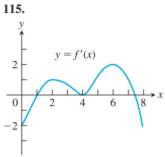
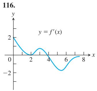
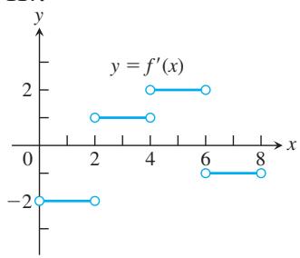
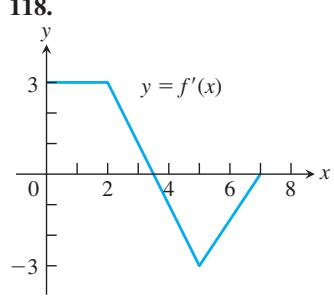
Solution (Integral) Curves
Exercises 119–122 show solution curves of differential equations. In each exercise, find an equation for the curve through the labeled point.
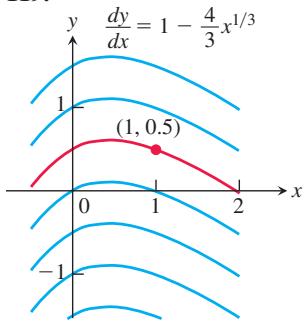
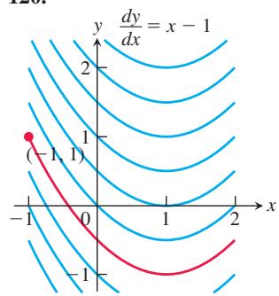
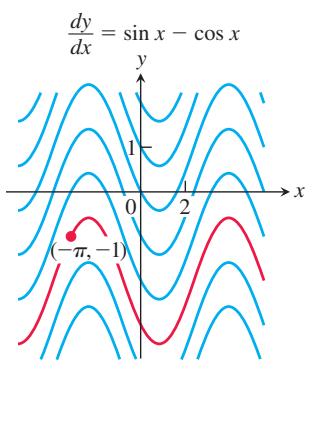
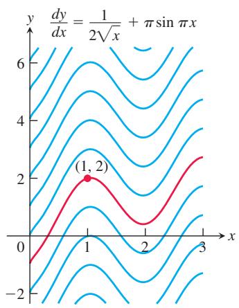
Applications
- Finding displacement from an antiderivative of velocity
a. Suppose that the velocity of a body moving along the s-axis is
i) Find the body’s displacement over the time interval from
ii) Find the body’s displacement from
iii) Now find the body’s displacement from
b. Suppose that the position
-
Liftoff from Earth A rocket lifts off the surface of Earth with a constant acceleration of
2 0 𝑚 / 𝑠 2 -
Stopping a car in time You are driving along a highway at a steady 108 km/h (30 m/s) when you see an accident ahead and slam on the brakes. What constant deceleration is required to stop your car in 75 m? To find out, carry out the following steps.
Step 1. Solve the initial value problem
Step 2. Find the value of
Step 3. Find the value of k that makes s = 75 for the value of t you found in Step 2.
-
Stopping a motorcycle The State of Illinois Cycle Rider Safety Program requires motorcycle riders to be able to brake from 48 km/h (13.3 m/s) to 0 in 13.7 m. What constant deceleration does it take to do that?
-
Motion along a coordinate line A particle moves on a coordinate line with acceleration
𝑎 = 𝑑 2 𝑠 / 𝑑 𝑡 2 = 1 5 √ 𝑡 − ( 3 / √ 𝑡 ) 𝑑 𝑠 / 𝑑 𝑡 = 4 𝑠 = 0 𝑡 = 1
a. the velocity
b. the position s in terms of t.
T 128. The hammer and the feather When Apollo 15 astronaut David Scott dropped a hammer and a feather on the moon to demonstrate that in a vacuum all bodies fall with the same (constant) acceleration, he dropped them from about 1.2 m above the ground. The television footage of the event shows the hammer and the feather falling more slowly than on Earth, where, in a vacuum, they would have taken only half a second to fall the 1.2 m. How long did it take the hammer and feather to fall 1.2 m on the moon? To find out, solve the following initial value problem for s as a function of t. Then find the value of t that makes s equal to 0.
Differential equation:
Initial conditions:
where
Differential equation:
Initial conditions:
where
Instead of using the result of Exercise 129, you can derive Equation (2) directly by solving an appropriate initial value problem. What initial value problem? Solve it to be sure you have the right one, explaining the solution steps as you go along.
- Suppose that
Find:
a.
c.
b.
e.
d.
f.
- Uniqueness of solutions If differentiable functions
𝑦 = 𝐹 ( 𝑥 ) 𝑦 = 𝑔 ( 𝑥 )
on an interval
COMPUTER EXPLORATIONS
Use a CAS to solve the initial value problems in Exercises 133–136. Plot the solution curves.
-
𝑦 ′ = c o s 2 𝑥 + s i n 𝑥 , 𝑦 ( 𝜋 ) = 1 -
𝑦 ′ = 1 𝑥 + 𝑥 , 𝑦 ( 1 ) = − 1 -
𝑦 ′ = 1 √ 4 − 𝑥 2 𝑦 ( 0 ) = 2 -
𝑦 ″ = 2 𝑥 + √ 𝑥 , 𝑦 ( 1 ) = 0 , 𝑦 ′ ( 1 ) = 0
CHAPTER 4 Questions to Guide Your Review
-
What can be said about the extreme values of a function that is continuous on a closed interval?
-
What does it mean for a function to have a local extreme value on its domain? An absolute extreme value? How are local and absolute extreme values related, if at all? Give examples.
-
How do you find the absolute extrema of a continuous function on a closed interval? Give examples.
-
What are the hypotheses and conclusion of Rolle’s Theorem? Are the hypotheses really necessary? Explain.
-
What are the hypotheses and conclusion of the Mean Value Theorem? What physical interpretations might the theorem have?
-
State the Mean Value Theorem’s three corollaries.
-
How can you sometimes identify a function
𝑓 ( 𝑥 ) 𝑓 ′ 𝑓 𝑥 = 𝑥 0 -
What is the First Derivative Test for Local Extreme Values? Give examples of how it is applied.
-
How do you test a twice-differentiable function to determine where its graph is concave up or concave down? Give examples.
-
What is an inflection point? Give an example. What physical significance do inflection points sometimes have?
-
What is the Second Derivative Test for Local Extreme Values? Give examples of how it is applied.
-
What do the derivatives of a function tell you about the shape of its graph?
-
List the steps you would take to graph a polynomial function. Illustrate with an example.
-
What is a cusp? Give examples.
-
List the steps you would take to graph a rational function. Illustrate with an example.
-
Outline a general strategy for solving max-min problems. Give examples.
-
Describe l’Hôpital’s Rule. How do you know when to use the rule and when to stop? Give an example.
-
How can you sometimes handle limits that lead to indeterminate forms
∞ / ∞ , ∞ ⋅ 0 ∞ − ∞ -
How can you sometimes handle limits that lead to indeterminate forms
1 ∞ , 0 0 ∞ ∞ -
Describe Newton’s method for solving equations. Give an example. What is the theory behind the method? What are some of the things to watch out for when you use the method?
-
Can a function have more than one antiderivative? If so, how are the antiderivatives related? Explain.
-
What is an indefinite integral? How do you evaluate one? What general formulas do you know for finding indefinite integrals?
-
How can you sometimes solve a differential equation of the form
𝑑 𝑦 / 𝑑 𝑥 = 𝑓 ( 𝑥 ) -
What is an initial value problem? How do you solve one? Give an example.
-
If you know the acceleration of a body moving along a coordinate line as a function of time, what more do you need to know to find the body’s position function? Give an example.
CHAPTER 4 Practice Exercises
Finding Extreme Values
In Exercises 1–16, find the extreme values (absolute and local) of the function over its natural domain, and where they occur.
-
𝑦 = 2 𝑥 2 − 8 𝑥 + 9 -
𝑦 = 𝑥 3 − 2 𝑥 + 4 -
𝑦 = 𝑥 3 + 𝑥 2 − 8 𝑥 + 5 -
𝑦 = 𝑥 3 ( 𝑥 − 5 ) 2 -
𝑦 = √ 𝑥 2 − 1 -
𝑦 = 𝑥 − 4 √ 𝑥 -
𝑦 = 1 3 √ 1 − 𝑥 2
-
𝑦 = 𝑥 𝑥 2 + 1 -
𝑦 = 𝑥 + 1 𝑥 2 + 2 𝑥 + 2 -
𝑦 = 𝑒 𝑥 + 𝑒 − 𝑥 -
𝑦 = 𝑒 𝑥 − 𝑒 − 𝑥 -
𝑦 = 𝑥 l n 𝑥 -
𝑦 = 𝑥 2 l n 𝑥 -
𝑦 = a r c c o s ( 𝑥 2 )
Extreme Values
-
Does
𝑓 ( 𝑥 ) = 𝑥 3 + 2 𝑥 + t a n 𝑥 -
Does
𝑔 ( 𝑥 ) = c s c 𝑥 + 2 c o t 𝑥 -
Does
𝑓 ( 𝑥 ) = ( 7 + 𝑥 ) ( 1 1 − 3 𝑥 ) 1 / 3 -
Find values of a and b such that the function
has a local extreme value of 1 at x = 3. Is this extreme value a local maximum or a local minimum? Give reasons for your answer.
-
Does
𝑔 ( 𝑥 ) = 𝑒 𝑥 − 𝑥 -
Does
𝑓 ( 𝑥 ) = 2 𝑒 𝑥 / ( 1 + 𝑥 2 ) 𝑓
In Exercises 23 and 24, find the absolute maximum and absolute minimum values of f over the interval.
-
𝑓 ( 𝑥 ) = 𝑥 − 2 l n 𝑥 , 1 ≤ 𝑥 ≤ 3 -
𝑓 ( 𝑥 ) = ( 4 / 𝑥 ) + l n 𝑥 2 , 1 ≤ 𝑥 ≤ 4 -
The greatest integer function
𝑓 ( 𝑥 ) = ⌊ 𝑥 ⌋ [ 0 , 1 ) -
a. Give an example of a differentiable function
𝑓 𝑐 𝑓 𝑐
b. How is this consistent with Theorem 2 in Section 4.1? Give reasons for your answer.
-
The function
𝑦 = 1 / 𝑥 0 < 𝑥 < 1 -
What are the maximum and minimum values of the function
𝑦 = | 𝑥 | − 1 ≤ 𝑥 < 1 -
A graph that is large enough to show a function’s global behavior may fail to reveal important local features. The graph of
𝑓 ( 𝑥 ) = ( 𝑥 8 / 8 ) − ( 𝑥 6 / 2 ) − 𝑥 5 + 5 𝑥 3
a. Graph f over the interval
b. Now factor
c. Zoom in on the graph to find a viewing window that shows the presence of the extreme values at
The moral here is that without calculus, the existence of two of the three extreme values would probably have gone unnoticed. On any normal graph of the function, the values would lie close enough together to fall within the dimensions of a single pixel on the screen.
(Source: Uses of Technology in the Mathematics Curriculum, by Benny Evans and Jerry Johnson, Oklahoma State University, published in 1990 under a grant from the National Science Foundation, USE-8950044.)
T 30. (Continuation of Exercise 29)
a. Graph
b. Show that
c. Zoom in to find a viewing window that shows the presence of the extreme values at
The Mean Value Theorem
- a. Show that
𝑔 ( 𝑡 ) = s i n 2 𝑡 − 3 𝑡
b. How many solutions does the equation
- a. Show that
𝑦 = t a n 𝜃
b. If the conclusion in part (a) is really correct, how do you explain the fact that
- a. Show that the equation
𝑥 4 + 2 𝑥 2 − 2 = 0 [ 0 , 1 ]
T b. Find the solution to as many decimal places as you can.
- a. Show that
𝑓 ( 𝑥 ) = 𝑥 / ( 𝑥 + 1 )
b. Show that
-
Water in a reservoir As a result of a heavy rain, the volume of water in a reservoir increased by million cubic meters in 24 hours. Show that at some instant during that period, the reservoir’s volume was increasing at a rate in excess of
5 0 0 , 0 0 0 L / m i n -
The formula
𝐹 ( 𝑥 ) = 3 𝑥 + 𝐶 𝐹 ′ ( 𝑥 ) = 3 -
Show that
even though
Doesn’t this contradict Corollary 2 of the Mean Value Theorem? Give reasons for your answer.
- Calculate the first derivatives of
𝑓 ( 𝑥 ) = 𝑥 2 / ( 𝑥 2 + 1 ) 𝑔 ( 𝑥 ) = − 1 / ( 𝑥 2 + 1 )
Analyzing Graphs
In Exercises 39 and 40, use the graph to answer the questions.
- Identify any global extreme values of
𝑓 𝑥
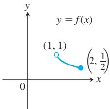
- Estimate the open intervals on which the function
𝑦 = 𝑓 ( 𝑥 )
a. increasing.
b. decreasing.
c. Use the given graph of
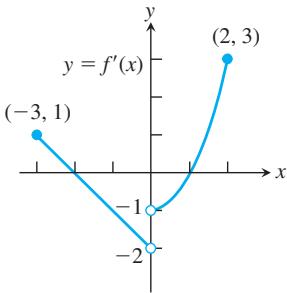
Each of the graphs in Exercises 41 and 42 is the graph of the position function
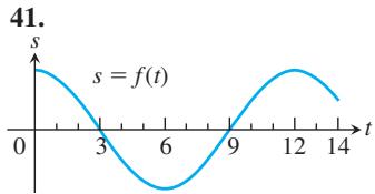
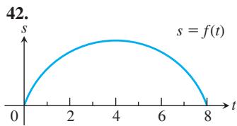
Graphs and Graphing
Graph the curves in Exercises 43–58.
-
𝑦 = 𝑥 2 − ( 𝑥 3 / 6 ) -
𝑦 = 𝑥 3 − 3 𝑥 2 + 3 -
𝑦 = − 𝑥 3 + 6 𝑥 2 − 9 𝑥 + 3 -
𝑦 = ( 1 / 8 ) ( 𝑥 3 + 3 𝑥 2 − 9 𝑥 − 2 7 ) -
𝑦 = 𝑥 3 ( 8 − 𝑥 ) -
𝑦 = 𝑥 2 ( 2 𝑥 2 − 9 ) -
𝑦 = 𝑥 − 3 𝑥 2 / 3 -
𝑦 = 𝑥 1 / 3 ( 𝑥 − 4 ) -
𝑦 = 𝑥 √ 3 − 𝑥 -
𝑦 = 𝑥 √ 4 − 𝑥 2 -
𝑦 = ( 𝑥 − 3 ) 2 𝑒 𝑥 -
𝑦 = 𝑥 𝑒 − 𝑥 2 -
𝑦 = l n ( 𝑥 2 − 4 𝑥 + 3 ) -
𝑦 = l n ( s i n 𝑥 ) -
𝑦 = a r c s i n ( 1 𝑥 ) -
𝑦 = t a n − 1 ( 1 𝑥 )
Each of Exercises 59–64 gives the first derivative of a function
-
𝑦 ′ = 1 6 − 𝑥 2 -
𝑦 ′ = 𝑥 2 − 𝑥 − 6 -
𝑦 ′ = 6 𝑥 ( 𝑥 + 1 ) ( 𝑥 − 2 ) -
𝑦 ′ = 𝑥 2 ( 6 − 4 𝑥 ) -
𝑦 ′ = 𝑥 4 − 2 𝑥 2 -
𝑦 ′ = 4 𝑥 2 − 𝑥 4
In Exercises 65–68, graph each function. Then use the function’s first derivative to explain what you see.
𝑦 = 𝑥 2 / 3 + ( 𝑥 − 1 ) 1 / 3
𝑦 = 𝑥 2 / 3 + ( 𝑥 − 1 ) 2 / 3
Sketch the graphs of the rational functions in Exercises 69–76.
-
𝑦 = 𝑥 + 1 𝑥 − 3 -
𝑦 = 2 𝑥 𝑥 + 5 -
𝑦 = 𝑥 2 + 1 𝑥 -
𝑦 = 𝑥 2 − 𝑥 + 1 𝑥 -
𝑦 = 𝑥 3 + 2 2 𝑥 -
𝑦 = 𝑥 4 − 1 𝑥 2 -
𝑦 = 𝑥 2 − 4 𝑥 2 − 3 -
𝑦 = 𝑥 2 𝑥 2 − 4
Using L’Hôpital’s Rule
Use l’Hôpital’s Rule to find the limits in Exercises 77–88.
-
l i m 𝑥 → 1 𝑥 2 + 3 𝑥 − 4 𝑥 − 1 -
l i m 𝑥 → 1 𝑥 𝑎 − 1 𝑥 𝑏 − 1 -
l i m 𝑥 → 𝜋 t a n 𝑥 𝑥 -
l i m 𝑥 → 0 t a n 𝑥 𝑥 + s i n 𝑥 -
l i m 𝑥 → 0 s i n 2 𝑥 t a n ( 𝑥 2 ) -
l i m 𝑥 → 0 s i n 𝑚 𝑥 s i n 𝑛 𝑥 -
l i m 𝑥 → 𝜋 / 2 − s e c 7 𝑥 c o s 3 𝑥 -
l i m 𝑥 → 0 + √ 𝑥 s e c 𝑥 -
l i m 𝑥 → 0 ( c s c 𝑥 − c o t 𝑥 ) -
l i m 𝑥 → 0 ( 1 𝑥 4 − 1 𝑥 2 ) -
l i m 𝑥 → ∞ ( √ 𝑥 2 + 𝑥 + 1 − √ 𝑥 2 − 𝑥 ) -
l i m 𝑥 → ∞ ( 𝑥 3 𝑥 2 − 1 − 𝑥 3 𝑥 2 + 1 )
Find the limits in Exercises 89–102.
-
l i m 𝑥 → 0 1 0 𝑥 − 1 𝑥 -
l i m 𝜃 → 0 3 𝜃 − 1 𝜃 -
l i m 𝑥 → 0 2 s i n 𝑥 − 1 𝑒 𝑥 − 1 -
l i m 𝑥 → 0 2 − s i n 𝑥 − 1 𝑒 𝑥 − 1 -
l i m 𝑥 → 0 5 − 5 c o s 𝑥 𝑒 𝑥 − 𝑥 − 1 -
l i m 𝑥 → 0 4 − 4 𝑒 𝑥 𝑥 𝑒 𝑥 -
l i m 𝑡 → 0 + 𝑡 − l n ( 1 + 2 𝑡 ) 𝑡 2 -
l i m 𝑥 → 4 s i n 2 ( 𝜋 𝑥 ) 𝑒 𝑥 − 4 + 3 − 𝑥 -
l i m 𝑡 → 0 + ( 𝑒 𝑡 𝑡 − 1 𝑡 ) -
l i m 𝑦 → 0 + 𝑒 − 1 / 𝑦 l n 𝑦 -
l i m 𝑥 → ∞ ( 1 + 𝑏 𝑥 ) 𝑘 𝑥 -
l i m 𝑥 → ∞ ( 1 + 2 𝑥 + 7 𝑥 2 ) -
l i m 𝑥 → 0 c o s 2 𝑥 − 1 − √ 1 − c o s 𝑥 s i n 2 𝑥 -
l i m 𝑥 → 0 √ 1 + t a n 𝑥 − √ 1 + s i n 𝑥 𝑥 3
Optimization
-
The sum of two nonnegative numbers is 36. Find the numbers if a. the difference of their square roots is to be as large as possible. b. the sum of their square roots is to be as large as possible.
-
The sum of two nonnegative numbers is 20. Find the numbers
a. if the product of one number and the square root of the other is to be as large as possible.
b. if one number plus the square root of the other is to be as large as possible.
-
An isosceles triangle has its vertex at the origin and its base parallel to the
𝑥 𝑦 = 2 7 − 𝑥 2 -
A customer has asked you to design an open-top rectangular stainless steel vat. It is to have a square base and a volume of
1 𝑚 3 -
Find the height and radius of the largest right circular cylinder that can be put in a sphere of radius
√ 3 -
The figure here shows two right circular cones, one upside down inside the other. The two bases are parallel, and the vertex of the smaller cone lies at the center of the larger cone’s base. What values of
𝑟 ℎ
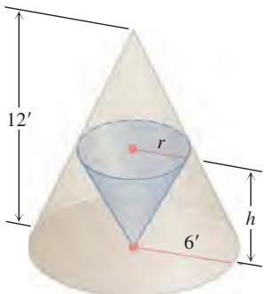
- Manufacturing tires Your company can manufacture x hundred grade A tires and y hundred grade B tires a day, where
0 ≤ 𝑥 ≤ 4
Your profit on a grade A tire is twice your profit on a grade B tire. What is the most profitable number of each kind to make?
- Particle motion The positions of two particles on the
𝑠 𝑠 1 = c o s 𝑡 𝑠 2 = c o s ( 𝑡 + 𝜋 / 4 )
a. What is the farthest apart the particles ever get?
b. When do the particles collide?
-
Open-top box An open-top rectangular box is constructed from a 25-cm-by-40-cm piece of cardboard by cutting squares of equal side length from the corners and folding up the sides. Find analytically the dimensions of the box of largest volume and the maximum volume. Support your answers graphically.
-
The ladder problem What is the approximate length (in meters) of the longest ladder you can carry horizontally around the corner of the corridor shown here? Round your answer down to the nearest meter.
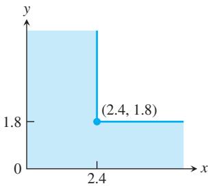
Newton’s Method
-
Let
𝑓 ( 𝑥 ) = 3 𝑥 − 𝑥 3 𝑓 ( 𝑥 ) = − 4 -
Let
𝑓 ( 𝑥 ) = 𝑥 4 − 𝑥 3 𝑓 ( 𝑥 ) = 7 5
Finding Indefinite Integrals
Find the indefinite integrals (most general antiderivatives) in Exercises 115–138. You may need to try a solution and then adjust your guess. Check your answers by differentiation.
-
∫ ( 𝑥 3 + 5 𝑥 − 7 ) 𝑑 𝑥 -
∫ ( 8 𝑡 3 − 𝑡 2 2 + 𝑡 ) 𝑑 𝑡 -
∫ ( 3 √ 𝑡 + 4 𝑡 2 ) 𝑑 𝑡 -
∫ ( 1 2 √ 𝑡 − 3 𝑡 4 ) 𝑑 𝑡 -
∫ 𝑑 𝑟 ( 𝑟 + 5 ) 2 -
∫ 6 𝑑 𝑟 ( 𝑟 − √ 2 ) 3 -
∫ 3 𝜃 √ 𝜃 2 + 1 𝑑 𝜃 -
∫ 𝜃 √ 7 + 𝜃 2 𝑑 𝜃 -
∫ 𝑥 3 ( 1 + 𝑥 4 ) − 1 / 4 𝑑 𝑥 -
∫ ( 2 − 𝑥 ) 3 / 5 𝑑 𝑥 -
∫ s e c 2 𝑠 1 0 𝑑 𝑠 -
∫ c s c 2 𝜋 𝑠 𝑑 𝑠 -
∫ c s c √ 2 𝜃 c o t √ 2 𝜃 𝑑 𝜃 -
∫ s e c 𝜃 3 t a n 𝜃 3 𝑑 𝜃 -
∫ s i n 2 𝑥 4 𝑑 𝑥 ( 𝐻 𝑖 𝑛 𝑡 : s i n 2 𝜃 = 1 − c o s 2 𝜃 2 ) -
∫ c o s 2 𝑥 2 𝑑 𝑥 -
∫ ( 3 𝑥 − 𝑥 ) 𝑑 𝑥 -
∫ ( 5 𝑥 2 + 2 𝑥 2 + 1 ) 𝑑 𝑥 -
∫ ( 1 2 𝑒 𝑡 − 𝑒 − 𝑡 ) 𝑑 𝑡 -
∫ ( 5 𝑠 + 𝑠 5 ) 𝑑 𝑠 -
∫ 𝜃 1 − 𝜋 𝑑 𝜃 -
∫ 2 𝜋 + 𝑟 𝑑 𝑟 -
∫ 3 2 𝑥 √ 𝑥 2 − 1 𝑑 𝑥 -
∫ 𝑑 𝜃 √ 1 6 − 𝜃 2
Initial Value Problems
Solve the initial value problems in Exercises 139–142.
-
𝑑 𝑦 𝑑 𝑥 = 𝑥 2 + 1 𝑥 2 , 𝑦 ( 1 ) = − 1 -
𝑑 𝑦 𝑑 𝑥 = ( 𝑥 + 1 𝑥 ) 2 , 𝑦 ( 1 ) = 1 -
𝑑 2 𝑟 𝑑 𝑡 2 = 1 5 √ 𝑡 + 3 √ 𝑡 ; 𝑟 ′ ( 1 ) = 8 , 𝑟 ( 1 ) = 0 -
𝑑 3 𝑟 𝑑 𝑡 3 = − c o s 𝑡 ; 𝑟 ″ ( 0 ) = 𝑟 ′ ( 0 ) = 0 , 𝑟 ( 0 ) = − 1
Applications and Examples
- Can the integrations in (a) and (b) both be correct? Explain.
- Can the integrations in (a) and (b) both be correct? Explain.
- The rectangle shown here has one side on the positive y-axis, one side on the positive x-axis, and its upper right-hand vertex on the curve
𝑦 = 𝑒 − 𝑥 2
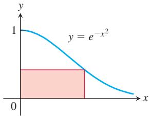
- The rectangle shown here has one side on the positive y-axis, one side on the positive x-axis, and its upper right-hand vertex on the curve
𝑦 = ( l n 𝑥 ) / 𝑥 2
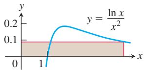
In Exercises 147 and 148, find the absolute maximum and minimum values of each function on the given interval.
-
𝑦 = 𝑥 l n 2 𝑥 − 𝑥 , [ 1 2 𝑒 , 𝑒 2 ] -
𝑦 = 1 0 𝑥 ( 2 − l n 𝑥 ) ( 0 , 𝑒 2 ]
In Exercises 149 and 150, find the absolute maxima and minima of the functions and give the x-coordinates where they occur.
-
𝑓 ( 𝑥 ) = 𝑒 𝑥 / √ 𝑥 4 + 1 -
𝑔 ( 𝑥 ) = 𝑒 √ 3 − 2 𝑥 − 𝑥 2
T 151. Graph the following functions and use what you see to locate and estimate the extreme values, identify the coordinates of the inflection points, and identify the intervals on which the graphs are concave up and concave down. Then confirm your estimates by working with the functions’ derivatives.
c.
T 152. Graph
T 153. Graph
- A round underwater transmission cable consists of a core of copper wires surrounded by nonconducting insulation. If x denotes the ratio of the radius of the core to the thickness of the insulation, it is known that the speed of the transmission signal is given by the equation
𝑣 = 𝑥 2 l n ( 1 / 𝑥 )
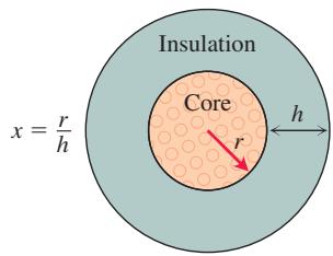
CHAPTER 4 Additional and Advanced Exercises
Functions and Derivatives
-
What can you say about a function whose maximum and minimum values on an interval are equal? Give reasons for your answer.
-
Is it true that a discontinuous function cannot have both an absolute maximum value and an absolute minimum value on a closed interval? Give reasons for your answer.
-
Can you conclude anything about the extreme values of a continuous function on an open interval? On a half-open interval? Give reasons for your answer.
-
Local extrema Use the sign pattern for the derivative
to identify the points where f has local maximum and minimum values.
5. Local extrema
a. Suppose that the first derivative of
At what points, if any, does the graph of f have a local maximum, local minimum, or point of inflection?
b. Suppose that the first derivative of
At what points, if any, does the graph of f have a local maximum, local minimum, or point of inflection?
-
If
𝑓 ′ ( 𝑥 ) ≤ 2 -
Bounding a function Suppose that
𝑓 [ 𝑎 , 𝑏 ] 𝑐 𝑓 ′ ( 𝑥 ) ≤ 0 [ 𝑎 , 𝑐 ) 𝑓 ′ ( 𝑥 ) ≥ 0 ( 𝑐 , 𝑏 ] 𝑓 ( 𝑥 ) 𝑓 ( 𝑐 ) [ 𝑎 , 𝑏 ]
8. An inequality
a. Show that
b. Suppose that
for any
-
The derivative of
𝑓 ( 𝑥 ) = 𝑥 2 𝑥 = 0 𝑓 -
Extrema and inflection points Let h = fg be the product of two differentiable functions of x.
a. If
b. If the graphs of
In either case, if the answer is yes, give a proof. If the answer is no, give a counterexample.
- Finding a function Use the following information to find the values of
𝑎 , 𝑏 𝑐 𝑓 ( 𝑥 ) = ( 𝑥 + 𝑎 ) / ( 𝑏 𝑥 2 + 𝑐 𝑥 + 2 ) 𝑎 , 𝑏 𝑐
b. The graph of
c. The line
- Horizontal tangent For what value or values of the constant k will the curve
𝑦 = 𝑥 3 + 𝑘 𝑥 2 + 3 𝑥 − 4
Optimization
-
Largest inscribed triangle Points A and B lie at the ends of a diameter of a unit circle and point C lies on the circumference. Is it true that the area of triangle ABC is largest when the triangle is isosceles? How do you know?
-
Proving the second derivative test The Second Derivative Test for Local Maxima and Minima (Section 4.4) says:
a.
b.
To prove statement (a), let
to conclude that for some
Thus,
- Hole in a water tank You want to bore a hole in the side of the tank shown here at a height that will make the stream of water coming out hit the ground as far from the tank as possible. If you drill the hole near the top, where the pressure is low, the water will exit slowly but spend a relatively long time in the air. If you drill the hole near the bottom, the water will exit at a higher velocity but have only a short time to fall. Where is the best place, if any, for the hole? (Hint: How long will it take an exiting droplet of water to fall from height y to the ground?)
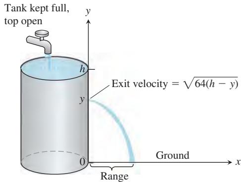
- Kicking a field goal An American football player wants to kick a field goal with the ball being on a right hash mark. Assume that the goal posts are b meters apart and that the hash mark line is a distance a > 0 meters from the right goal post. (See the accompanying figure.) Find the distance h from the goal post line that gives the kicker his largest angle
𝛽
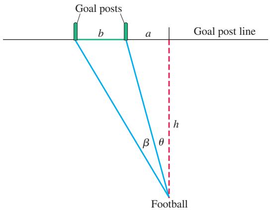
- A max-min problem with a variable answer Sometimes the solution of a max-min problem depends on the proportions of the shapes involved. As a case in point, suppose that a right circular cylinder of radius
𝑟 ℎ 𝑅 𝐻 𝑟 𝑅 𝐻 𝐻 ≤ 2 𝑅 𝐻 > 2 𝑅
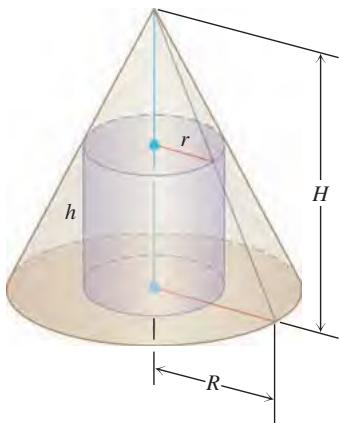
-
Minimizing a parameter Find the smallest value of the positive constant m that will make
𝑚 𝑥 − 1 + ( 1 / 𝑥 ) -
Determine the dimensions of the rectangle of largest area that can be inscribed in the right triangle in the accompanying figure.
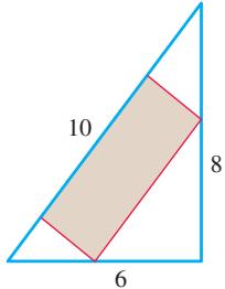
- A rectangular box with a square base is inscribed in a right circular cone of height 4 and base radius 3. If the base of the box sits on the base of the cone, what is the largest possible volume of the box?
Limits
-
Evaluate the following limits. a.
l i m 𝑥 → 0 2 s i n 5 𝑥 3 𝑥 l i m 𝑥 → 0 s i n 5 𝑥 c o t 3 𝑥 l i m 𝑥 → 0 𝑥 c s c 2 √ 2 𝑥 l i m 𝑥 → 𝜋 / 2 ( s e c 𝑥 − t a n 𝑥 ) l i m 𝑥 → 0 𝑥 − s i n 𝑥 𝑥 − t a n 𝑥 l i m 𝑥 → 0 s i n 𝑥 2 𝑥 s i n 𝑥 l i m 𝑥 → 0 s e c 𝑥 − 1 𝑥 2 l i m 𝑥 → 2 𝑥 3 − 8 𝑥 2 − 4 -
L’Hôpital’s Rule does not help with the following limits. Find them some other way. a.
l i m 𝑥 → ∞ √ 𝑥 + 5 √ 𝑥 + 5 l i m 𝑥 → ∞ 2 𝑥 𝑥 + 7 √ 𝑥
Theory and Examples
-
Suppose that it costs a company
𝑦 = 𝑎 + 𝑏 𝑥 -
Estimating reciprocals without division You can estimate the value of the reciprocal of a number
𝑎 𝑎 𝑓 ( 𝑥 ) = ( 1 / 𝑥 ) − 𝑎 𝑎 = 3 𝑓 ( 𝑥 ) = ( 1 / 𝑥 ) − 3 𝑦 = ( 1 / 𝑥 ) − 3 𝑥
b. Show that the recursion formula in this case is
so there is no need for division.
- To find
𝑥 = 𝑞 √ 𝑎 𝑓 ( 𝑥 ) = 𝑥 𝑞 − 𝑎 𝑎 𝑞 𝑥 1 𝑥 0 𝑎 / 𝑥 𝑞 − 1 0 𝑚 0 , 𝑚 1
What conclusion would you reach if
- The family of straight lines
𝑦 = 𝑎 𝑥 + 𝑏 𝑦 ″ = 0
where h and r are arbitrary constants. (Hint: Eliminate h and r from the set of three equations including the given one and two obtained by successive differentiation.)
-
Free fall in the fourteenth century In the middle of the fourteenth century, Albert of Saxony (1316–1390) proposed a model of free fall, which assumed that the velocity of a falling body was proportional to the distance fallen. It seemed reasonable to think that a body that had fallen 6 m might be moving twice as fast as a body that had fallen 3 m. And besides, none of the instruments in use at the time were accurate enough to prove otherwise. Today we can see just how far off Albert of Saxony’s model was by solving the initial value problem implicit in his model. Solve the problem and compare your solution graphically with the equation
𝑠 = 4 . 9 𝑡 2 -
Group testing During World War II it was necessary to administer blood tests to large numbers of recruits. There are two standard ways to administer a blood test to N people. In method 1, each person is tested separately. In method 2, the blood samples of x people are pooled and tested as one large sample. If the test is negative, this one test is enough for all x people. If the test is positive, then each of the x people is tested separately, requiring a total of
𝑥 + 1
With q = 0.99 and N = 1000, find the integer value of x that minimizes y. Also find the integer value of x that maximizes y. (This second result is not important to the real-life situation.) The group testing method was used in World War II with a savings of 80% over the individual testing method, but not with the given value of q. Group testing has been implemented in diagnosing various diseases, including COVID-19.
-
Assume that the brakes of an automobile produce a constant deceleration of
𝑘 𝑚 / 𝑠 2 -
Let
𝑓 ( 𝑥 ) 𝑔 ( 𝑥 ) 𝑓 ′ ( 𝑥 ) = 𝑔 ( 𝑥 ) 𝑓 ″ ( 𝑥 ) = − 𝑓 ( 𝑥 ) ℎ ( 𝑥 ) = 𝑓 2 ( 𝑥 ) + 𝑔 2 ( 𝑥 ) ℎ ( 0 ) = 5 ℎ ( 1 0 ) -
Can there be a curve satisfying the following conditions?
𝑑 2 𝑦 / 𝑑 𝑥 2 𝑥 = 0 , 𝑦 = 0 𝑑 𝑦 / 𝑑 𝑥 = 1 -
Find the equation for the curve in the
𝑥 𝑦 ( 1 , − 1 ) 𝑥 3 𝑥 2 + 2 -
A particle moves along the x-axis. Its acceleration is
𝑎 = − 𝑡 2 -
A particle moves with acceleration
𝑎 = √ 𝑡 − ( 1 / √ 𝑡 )
a. the velocity v in terms of t.
b. the position s in terms of t.
-
Given
𝑓 ( 𝑥 ) = 𝑎 𝑥 2 + 2 𝑏 𝑥 + 𝑐 𝑎 > 0 𝑓 ( 𝑥 ) ≥ 0 𝑥 𝑏 2 − 𝑎 𝑐 ≤ 0 -
The Cauchy–Schwarz inequality
a. In Exercise 35, let
and deduce The Cauchy–Schwarz inequality:
b. Show that equality holds in The Cauchy–Schwarz inequality only if there exists a real number x that makes
- The best branching angles for blood vessels and pipes When a smaller pipe branches off from a larger one in a flow system, we may want it to run off at an angle that is best from some energy-saving point of view. We might require, for instance, that energy loss due to friction be minimized along the section AOB shown in the accompanying figure. In this diagram, B is a given point to be reached by the smaller pipe, A is a point in the larger pipe upstream from B, and O is the point where the branching occurs. A law formulated by Poiseuille states that the loss of energy due to friction in nonturbulent flow is proportional to the length of the path and inversely proportional to the fourth power of the radius. Thus, the loss along AO is
( 𝑘 𝑑 1 ) / 𝑅 4 ( 𝑘 𝑑 2 ) / 𝑟 4 𝑑 1 𝑑 2 𝜃
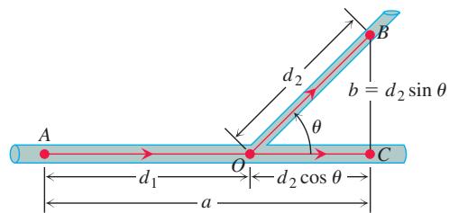
In our model, we assume that
We can express the total loss L as a function of
so that
a. Show that the critical value of
b. If the ratio of the pipe radii is r/R = 5/6 estimate to the nearest degree the optimal branching angle given in part (a).
- Consider point
( 𝑎 , 𝑏 ) 𝑦 = l n 𝑥 ( 𝑎 , 𝑏 )
Mathematica/Maple Projects
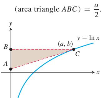
- Consider the unit circle centered at the origin and with a vertical tangent line passing through point
𝐴 𝐴 𝐵 𝐴 𝐶 𝐷 𝑥 𝐵 𝐶 𝑡 𝐵 𝐴
Projects can be found within MyLab Math.
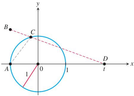
CHAPTER 4 Technology Application Projects
- Motion Along a Straight Line: Position → Velocity → Acceleration
You will observe the shape of a graph through dramatic animated visualizations of the derivative relations among the position, velocity, and acceleration. Figures in the text can be animated.
- Newton’s Method: Estimate
𝜋
Plot a function, observe a root, pick a starting point near the root, and use Newton’s Iteration Procedure to approximate the root to a desired accuracy. The numbers