Chapter 7: Integrals and Transcendental Functions

7.1 The Logarithm Defined as an Integral

In Chapter 1, we introduced the natural logarithm function $l n 𝑥$ as the inverse of the exponential function $𝑒 𝑥$ . The function $𝑒 𝑥$ was chosen as that function in the family of general exponential functions $𝑎 𝑥, 𝑎 > 0$ , whose graph has slope 1 as it crosses the $𝑦$ -axis. The function $𝑎 𝑥$ was presented intuitively, however, based on its graph at rational values of $𝑥$ .

In this section we recreate the theory of logarithmic and exponential functions from an entirely different point of view. Here we define these functions analytically and derive their behaviors. To begin, we use the Fundamental Theorem of Calculus to define the natural logarithm function $l n 𝑥$ as an integral. We quickly develop its properties, including the algebraic, geometric, and analytic properties with which we are already familiar. Next we introduce the function $𝑒 𝑥$ as the inverse function of $l n 𝑥$ , and establish its properties. Defining $l n 𝑥$ as an integral and $𝑒 𝑥$ as its inverse is an indirect approach that gives an elegant and powerful way to obtain and validate the key properties of logarithmic and exponential functions.

Definition of the Natural Logarithm Function

The natural logarithm of a positive number x, written as $l n 𝑥$ , is the value of an integral. The appropriate integral is suggested by our earlier results in Chapter 5.

DEFINITION The natural logarithm is the function given by
$l n 𝑥 = \int 𝑥 1 1 𝑡 𝑑 𝑡, 𝑥 > 0 .$

From the Fundamental Theorem of Calculus, we know that $l n 𝑥$ is a continuous function. Geometrically, if x > 1, then $l n 𝑥$ is the area under the curve y = 1/t from t = 1 to t = x (Figure 7.1). For 0 < x < 1, $l n 𝑥$ gives the negative of the area under the curve from x to 1, and the function is not defined for $𝑥 \leq 0$ . From the Zero Width Interval Rule for definite integrals, we also have

l n 1 = \int 11 1 𝑡 𝑑 𝑡 = 0 .

教材插图

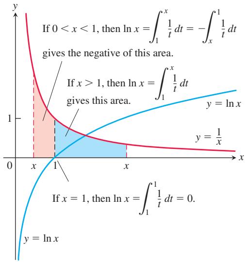
FIGURE 7.1 The graph of $𝑦 = l n 𝑥$ and its relation to the function $𝑦 = 1 / 𝑥, 𝑥 > 0$ . The graph of the logarithm rises above the x-axis as x moves from 1 to the right, and it falls below the axis as x moves from 1 to the left.

Notice that we show the graph of $𝑦 = 1 / 𝑥$ in Figure 7.1 but use $𝑦 = 1 / 𝑡$ in the integral. Using $𝑥$ for everything would have us writing

TABLE 7.1 Typical 2-place values of ln x

x	ln x
0	undefined
0.05	-3.00
0.5	-0.69
1	0
2	0.69
3	1.10
4	1.39
10	2.30

l n 𝑥 = \int 𝑥 1 1 𝑥 𝑑 𝑥,

with $𝑥$ meaning two different things. So we change the variable of integration to $𝑡$ .

By using rectangles to obtain finite approximations of the area under the graph of $𝑦 = 1 / 𝑡$ and over the interval between $𝑡 = 1$ and $𝑡 = 𝑥$ , as in Section 5.1, we can approximate the values of the function $l n 𝑥$ . Several values are given in Table 7.1. There is an important number between $𝑥 = 2$ and $𝑥 = 3$ whose natural logarithm equals 1. This number, which we now define, exists because $l n 𝑥$ is a continuous function and therefore satisfies the Intermediate Value Theorem on the interval [2, 3].

DEFINITION The number e is the number in the domain of the natural logarithm that satisfies
$l n (𝑒) = \int 𝑒 1 1 𝑡 𝑑 𝑡 = 1 .$

Interpreted geometrically, the number e corresponds to the point on the x-axis for which the area under the graph of y = 1/t and above the interval $[1, 𝑒]$ equals the area of the unit square. That is, the area of the region shaded blue in Figure 7.1 is 1 square unit when x = e. We will see further on that this is the same number $𝑒 \approx 2.718281828$ we have encountered before.

The Derivative of $𝑦 = l n 𝑥$

By the first part of the Fundamental Theorem of Calculus (Section 5.4),

𝑑 𝑑 𝑥 l n 𝑥 = 𝑑 𝑑 𝑥 \int 𝑥 1 1 𝑡 𝑑 𝑡 = 1 𝑥,

so we have

𝑑 𝑑 𝑥 l n 𝑥 = 1 𝑥, 𝑥 > 0 . (1)

Therefore, the function $𝑦 = l n 𝑥$ is a solution to the initial value problem $𝑑 𝑦 / 𝑑 𝑥 = 1 / 𝑥$ , $𝑥 > 0$ , with $𝑦 (1) = 0$ . Notice that the derivative is always positive.

If $𝑢$ is a differentiable function of $𝑥$ whose values are positive so that $l n 𝑢$ is defined, then by applying the Chain Rule, we obtain

𝑑 𝑑 𝑥 l n 𝑢 = 1 𝑢 𝑑 𝑢 𝑑 𝑥, 𝑢 > 0 . (2)

The derivative of $l n | 𝑥 |$ can be found just as in Example 3(c) of Section 3.8, giving

(3)

教材插图

(a)

𝑑 𝑑 𝑥 l n | 𝑥 | = 1 𝑥, 𝑥 \neq 0 .

教材插图

(b)

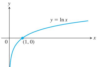
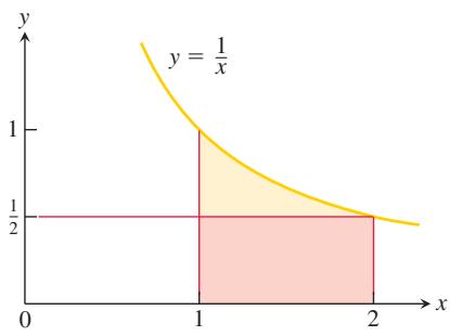
FIGURE 7.2 (a) The graph of the natural logarithm. (b) The rectangle of height y = 1/2 fits beneath the graph of y = 1/x for the interval $1 \leq 𝑥 \leq 2$ .

Moreover, if b is any constant with bx > 0, Equation (2) gives

𝑑 𝑑 𝑥 l n 𝑏 𝑥 = 1 𝑏 𝑥 \cdot 𝑑 𝑑 𝑥 (𝑏 𝑥) = 1 𝑏 𝑥 (𝑏) = 1 𝑥 .

The Graph and Range of $l n 𝑥$

The derivative $𝑑 (l n 𝑥) / 𝑑 𝑥 = 1 / 𝑥$ is positive for x > 0, so $l n 𝑥$ is an increasing function of x. The second derivative, $- 1 / 𝑥 2$ , is negative, so the graph of $l n 𝑥$ is concave down. (See Figure 7.2a.)

The function $l n 𝑥$ has the following familiar algebraic properties, which we stated in Section 1.5. In Section 4.2 we showed these properties are a consequence of Corollary 2 of the Mean Value Theorem, and those derivations still apply.

$l n 𝑏 𝑥 = l n 𝑏 + l n 𝑥$

l n 𝑏 𝑥 = l n 𝑏 - l n 𝑥

$l n 1 𝑥 = - l n 𝑥$
$l n 𝑥 𝑟 = 𝑟 l n 𝑥, 𝑟$ rational

We can estimate the value of $l n 2$ by considering the area under the graph of y = 1/x and above the interval [1, 2]. In Figure 7.2(b) a rectangle of height 1/2 over the interval [1, 2] fits under the graph. Therefore, the area under the graph, which is ln 2, is greater than the area of the rectangle, which is 1/2. So ln 2 > 1/2. Knowing this we have

l n 2 𝑛 = 𝑛 l n 2 > 𝑛 (12) = 𝑛 2 .

This result shows that $l n (2 𝑛) \to \infty$ as $𝑛 \to \infty$ . Since $l n 𝑥$ is an increasing function, it follows that

l i m 𝑥 \to \infty l n 𝑥 = \infty . I n 𝑥 i s i n c r e a s i n g a n d n o t b o u n d e d a b o v e .

We also have

l i m 𝑥 \to 0 + l n 𝑥 = l i m 𝑡 \to \infty l n 1 𝑡 = l i m 𝑡 \to \infty (- l n 𝑡) = - \infty . 𝑥 = 1 / 𝑡

We defined $l n 𝑥$ for x > 0, so the domain of $l n 𝑥$ is the set of positive real numbers. The above discussion and the Intermediate Value Theorem show that its range is the entire real line, giving the familiar graph of $𝑦 = l n 𝑥$ shown in Figure 7.2(a).

The Integral $\int 1 / 𝑥 𝑑 𝑥$

Equation (3) leads to the following integral formula:

\int 1 𝑥 𝑑 𝑥 = l n | 𝑥 | + 𝐶 . (4)

If u is a differentiable function that is never zero, then

\int 1 𝑢 𝑑 𝑢 = l n | 𝑢 | + 𝐶 . (5)

Equation (5) applies anywhere on the domain of $1 / 𝑢$ , which is the set of points where $𝑢 \neq 0$ . It says that integrals that have the form $\int 𝑑 𝑢 𝑢$ lead to logarithms. Whenever $𝑢 = 𝑓 (𝑥)$ is a differentiable function that is never zero, we have that $𝑑 𝑢 = 𝑓' (𝑥) 𝑑 𝑥$ and

\int 𝑓' (𝑥) 𝑓 (𝑥) 𝑑 𝑥 = l n | 𝑓 (𝑥) | + 𝐶 .

EXAMPLE 1 We rewrite an integral so that it has the form $\int 𝑑 𝑢 𝑢$ .

\int 𝜋 / 2 - 𝜋 / 2 4 c o s 𝜃 3 + 2 s i n 𝜃 𝑑 𝜃 = \int 51 2 𝑢 𝑑 𝑢 = 2 l n | 𝑢 | ∣ 51 = 2 l n | 5 | - 2 l n | 1 | = 2 l n 5 𝑢 = 3 + 2 s i n 𝜃, 𝑑 𝑢 = 2 c o s 𝜃 𝑑 𝜃, 𝑢 (- 𝜋 / 2) = 1, 𝑢 (𝜋 / 2) = 5

Note that $𝑢 = 3 + 2 s i n 𝜃$ is always positive on $[- 𝜋 / 2, 𝜋 / 2]$ , so Equation (5) applies.

The Inverse of $l n 𝑥$ and the Number $𝑒$

The function $l n 𝑥$ , being an increasing function of x with domain $(0, \infty)$ and range $(- \infty, \infty)$ , has an inverse $l n - 1 𝑥$ with domain $(- \infty, \infty)$ and range $(0, \infty)$ . The graph of $l n - 1 𝑥$ is the graph of $l n 𝑥$ reflected across the line y = x. As you can see in Figure 7.3,

l i m 𝑥 \to \infty l n - 1 𝑥 = \infty a n d l i m 𝑥 \to - \infty l n - 1 𝑥 = 0 .

教材插图

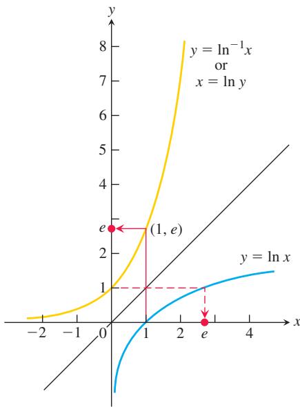
FIGURE 7.3 The graphs of $𝑦 = l n 𝑥$ and $𝑦 = l n - 1 𝑥 = e x p 𝑥$ . The number $𝑒$ is $l n - 1 1 = e x p (1)$ .

The notations $l n - 1 𝑥$ , $e x p 𝑥$ , and $𝑒 𝑥$ all refer to the natural exponential function.

Typical values of $𝑒 𝑥$

x	ex(rounded)
-1	0.37
0	1
1	2.72
2	7.39
10	22026
100	$2.6881 \times 1043$

The inverse function $l n - 1 𝑥$ is also denoted by $e x p 𝑥$ . We have not yet established that $e x p 𝑥$ is an exponential function, only that $e x p 𝑥$ is the inverse of the function $l n 𝑥$ . We will now show that $l n - 1 𝑥 = e x p 𝑥$ is, in fact, the exponential function with base e.

The number e was defined to satisfy the equation $l n (𝑒) = 1$ , so $𝑒 = e x p (1)$ . We can raise the number e to a rational power r using algebra:

𝑒 2 = 𝑒 \cdot 𝑒, 𝑒 - 2 = 1 𝑒 2, 𝑒 1 / 2 = \sqrt 𝑒, 𝑒 2 / 3 = 3 \sqrt 𝑒 2,

and so on. Since e is positive, $𝑒 𝑟$ is positive too. Therefore, $𝑒 𝑟$ has a logarithm. When we take the logarithm, we find that if r is rational, then

l n 𝑒 𝑟 = 𝑟 l n 𝑒 = 𝑟 \cdot 1 = 𝑟 .

Applying the function $l n - 1$ to both sides of the equation $l n 𝑒 𝑟 = 𝑟$ , we find that

𝑒 𝑟 = e x p 𝑟 f o r 𝑟 r a t i o n a l . e x p i s l n - 1 . (6)

Thus exp r coincides with the exponential function $𝑒 𝑟$ for all rational values of r. We have not yet found a way to give an exact meaning to $𝑒 𝑥$ for x irrational, but we can use Equation (6) to do so. The function $e x p 𝑥 = l n - 1 𝑥$ has domain $(- \infty, \infty)$ , so it is defined for every x. We have $e x p 𝑟 = 𝑒 𝑟$ for r rational by Equation (6), and we now define $𝑒 𝑥$ to equal $e x p 𝑥$ for all x.

DEFINITION For every real number $𝑥$ , we define the natural exponential function to be $𝑒 𝑥 = e x p 𝑥$ .

For the first time we have a precise meaning for a number raised to an irrational power. Usually the exponential function is denoted by $𝑒 𝑥$ rather than $e x p 𝑥$ . Since $l n 𝑥$ and $𝑒 𝑥$ are inverses of one another, we have the following relations.

Inverse Equations for $𝑒 𝑥$ and $l n 𝑥$

𝑒 l n 𝑥 = 𝑥 (a l l x > 0) l n (𝑒 𝑥) = 𝑥 (a l l x)

The Derivative and Integral of $𝑒 𝑥$

The exponential function is differentiable because it is the inverse of a differentiable function whose derivative is never zero. We calculate its derivative by using Theorem 3 of Section 3.8 and our knowledge of the derivative of $l n 𝑥$ . Let

𝑓 (𝑥) = l n 𝑥 a n d 𝑦 = 𝑒 𝑥 = l n - 1 𝑥 = 𝑓 - 1 (𝑥) .

Then

𝑑 𝑦 𝑑 𝑥 = 𝑑 𝑑 𝑥 𝑒 𝑥 = 𝑑 𝑑 𝑥 l n - 1 𝑥 = 𝑑 𝑑 𝑥 𝑓 - 1 (𝑥) = 1 𝑓' (𝑓 - 1 (𝑥)) T h e o r e m 3, S e c t i o n 3.8 = 1 𝑓' (𝑒 𝑥) 𝑓 - 1 (𝑥) = 𝑒 𝑥 = 1 (1 𝑒 𝑥) 𝑓' (𝑧) = 1 𝑧 w i t h 𝑧 = 𝑒 𝑥 = 𝑒 𝑥 .

That is, for $𝑦 = 𝑒 𝑥$ , we find that $𝑑 𝑦 / 𝑑 𝑥 = 𝑒 𝑥$ , so the natural exponential function $𝑒 𝑥$ is its own derivative, just as we claimed in Section 3.3.

𝑑 𝑑 𝑥 𝑒 𝑥 = 𝑒 𝑥 . (7)

We will see in the next section that the only functions that behave this way are constant multiples of $𝑒 𝑥$ . The Chain Rule extends the derivative result in the usual way to a more general form: If u is any differentiable function of x, then

𝑑 𝑑 𝑥 𝑒 𝑢 = 𝑒 𝑢 𝑑 𝑢 𝑑 𝑥 . (8)

Since $𝑒 𝑥 > 0$ , its derivative is also everywhere positive, so it is an increasing and continuous function for all $𝑥$ , having limits

l i m 𝑥 \to - \infty 𝑒 𝑥 = 0 a n d l i m 𝑥 \to \infty 𝑒 𝑥 = \infty .

It follows that the $𝑥$ -axis $(𝑦 = 0)$ is a horizontal asymptote of the graph $𝑦 = 𝑒 𝑥$ (see Figure 7.3).

Equation (7) also tells us the indefinite integral of $𝑒 𝑥$ .

\int 𝑒 𝑥 𝑑 𝑥 = 𝑒 𝑥 + 𝐶

If $𝑓 (𝑥) = 𝑒 𝑥$ , then we see from Equation (7) that $𝑓' (0) = 𝑒 0 = 1$ . That is, the exponential function $𝑒 𝑥$ has slope 1 as it crosses the y-axis at x = 0. This agrees with our assertion for the natural exponential in Section 3.3.

Logarithms and Laws of Exponents

The familiar algebraic properties of logarithms and exponential functions were stated in Section 1.5. We now show that these follow from the definition of the logarithm as an integral that we have used. The properties of logarithms are stated in Theorem 1.

THEOREM 1—Algebraic Properties of the Natural Logarithm

For any numbers $𝑏 > 0$ and $𝑥 > 0$ , the natural logarithm satisfies the following rules:

Product Rule:

l n 𝑏 𝑥 = l n 𝑏 + l n 𝑥

Quotient Rule:

l n 𝑏 𝑥 = l n 𝑏 - l n 𝑥

Reciprocal Rule:

l n 1 𝑥 = - l n 𝑥

R u l e 2 w i t h 𝑏 = 1

Power Rule:

l n 𝑥 𝑟 = 𝑟 l n 𝑥

The proof uses the Mean Value Theorem, which was established in Section 4.2.

Proof that $l n 𝑏 𝑥 = l n 𝑏 + l n 𝑥$ The argument starts by observing that $l n 𝑏 𝑥$ and $l n 𝑥$ have the same derivative:

𝑑 𝑑 𝑥 l n (𝑏 𝑥) = 𝑏 𝑏 𝑥 = 1 𝑥 = 𝑑 𝑑 𝑥 l n 𝑥 .

According to Corollary 2 of the Mean Value Theorem, the functions must differ by a constant, which means that

l n 𝑏 𝑥 = l n 𝑥 + 𝐶

for some $𝐶$ .

Since this last equation holds for all positive values of x, it must hold for x = 1. Hence,

l n (𝑏 \cdot 1) = l n 1 + 𝐶 l n 𝑏 = 0 + 𝐶 l n 1 = 0 𝐶 = l n 𝑏 .

By substituting, we conclude

l n 𝑏 𝑥 = l n 𝑏 + l n 𝑥 .

Proof that $l n 𝑥 𝑟 = 𝑟 l n 𝑥$ We use the same-derivative argument again. For all positive values of x,

𝑑 𝑑 𝑥 l n 𝑥 𝑟 = 1 𝑥 𝑟 𝑑 𝑑 𝑥 (𝑥 𝑟) C h a i n R u l e = 1 𝑥 𝑟 𝑟 𝑥 𝑟 - 1 D e r i v a t i v e P o w e r R u l e = 𝑟 \cdot 1 𝑥 = 𝑑 𝑑 𝑥 (𝑟 l n 𝑥) .

Since $l n 𝑥 𝑟$ and $𝑟 l n 𝑥$ have the same derivative,

l n 𝑥 𝑟 = 𝑟 l n 𝑥 + 𝐶

for some constant C. Taking x to be 1 identifies C as zero, and we’re done.

You are asked to prove the Quotient Rule for logarithms,

l n (𝑏 𝑥) = l n 𝑏 - l n 𝑥,

in Exercises 63. The Reciprocal Rule, $l n (1 / 𝑥) = - l n 𝑥$ , is a special case of the Quotient Rule, obtained by taking $𝑏 = 1$ and noting that $l n 1 = 0$ .

We now state the algebraic properties of exponential functions.

THEOREM 2—Laws of Exponents for $𝑒 𝑥$

For all numbers x and y, the natural exponential function $𝑒 𝑥$ obeys the following laws.

1 . 𝑒 𝑥 𝑒 𝑦 = 𝑒 𝑥 + 𝑦

2 . 𝑒 - 𝑥 = 1 𝑒 𝑥

3 . 𝑒 𝑥 𝑒 𝑦 = 𝑒 𝑥 - 𝑦

4 . (𝑒 𝑥) 𝑦 = 𝑒 𝑥 𝑦 = (𝑒 𝑦) 𝑥

Proof that $𝑒 𝑥 𝑒 𝑦 = 𝑒 𝑥 + 𝑦$

𝑒 𝑥 𝑒 𝑦 = 𝑒 l n (𝑒 𝑥 𝑒 𝑦) 𝑢 = 𝑒 l n 𝑢 . = 𝑒 l n (𝑒 𝑥) + l n (𝑒 𝑦) P r o d u c t f o r m u l a f o r l n = 𝑒 𝑥 + 𝑦 . l n 𝑒 𝑢 = 𝑢 .

Theorem 1 and the inverse relationship between the logarithmic and exponential functions also imply the other algebraic properties of the exponential function (see Exercise 67).

The General Exponential Function $𝑎 𝑥$

Since $𝑎 = 𝑒 l n 𝑎$ for any positive number $𝑎$ , we can express $𝑎 𝑥$ as $(𝑒 l n 𝑎) 𝑥 = 𝑒 𝑥 l n 𝑎$ . We therefore make the following definition, consistent with what we stated in Section 1.5.

DEFINITION For any numbers a > 0 and x, the exponential function with base a is given by
$𝑎 𝑥 = 𝑒 𝑥 l n 𝑎 .$

The General Power Function

$𝑥 𝑟$ is the function $𝑒 𝑟 l n 𝑥$ .

When a = e, the definition gives $𝑎 𝑥 = 𝑒 𝑥 l n 𝑎 = 𝑒 𝑥 l n 𝑒 = 𝑒 𝑥 \cdot 1 = 𝑒 𝑥$ . Similarly, the power function $𝑓 (𝑥) = 𝑥 𝑟$ is defined for positive x by the formula $𝑥 𝑟 = 𝑒 𝑟 l n 𝑥$ , which holds for any real number r, rational or irrational.

Theorem 2 is also valid for $𝑎 𝑥$ , the exponential function with base a. For example,

𝑎 𝑥 \cdot 𝑎 𝑦 = 𝑒 𝑥 l n 𝑎 \cdot 𝑒 𝑦 l n 𝑎 D e f i n i t i o n o f 𝑎 𝑥 = 𝑒 𝑥 l n 𝑎 + 𝑦 l n 𝑎 L a w 1 = 𝑒 (𝑥 + 𝑦) l n 𝑎 C o m m o n f a c t o r l n 𝑎 = 𝑎 𝑥 + 𝑦 . D e f i n i t i o n o f 𝑎 𝑥

Starting with the definition $𝑎 𝑥 = 𝑒 𝑥 l n 𝑎, 𝑎 > 0$ , we get the derivative

𝑑 𝑑 𝑥 𝑎 𝑥 = 𝑑 𝑑 𝑥 𝑒 𝑥 l n 𝑎 = (l n 𝑎) 𝑒 𝑥 l n 𝑎 = (l n 𝑎) 𝑎 𝑥,

𝑑 𝑑 𝑥 𝑎 𝑥 = 𝑎 𝑥 l n 𝑎 .

Alternatively, we get the same derivative rule by applying logarithmic differentiation:

𝑦 = 𝑎 𝑥

Take logarithms.

1 𝑦 𝑑 𝑦 𝑑 𝑥 = l n 𝑎

Differentiate with respect to $𝑥$ .

𝑑 𝑦 𝑑 𝑥 = 𝑦 l n 𝑎 = 𝑎 𝑥 l n 𝑎 .

With the Chain Rule, we get a more general form, as in Section 3.8: If $𝑎 > 0$ and $𝑢$ is a differentiable function of $𝑥$ , then $𝑎 𝑢$ is a differentiable function of $𝑥$ and

𝑑 𝑑 𝑥 𝑎 𝑢 = 𝑎 𝑢 l n 𝑎 𝑑 𝑢 𝑑 𝑥 .

教材插图

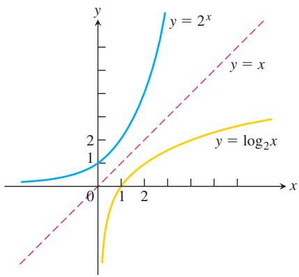
FIGURE 7.4 The graph of $2 𝑥$ and its inverse, $l o g 2 𝑥$ .

TABLE 7.2 Rules for base a logarithms

For any numbers $𝑥 > 0$ and $𝑦 > 0$ ,

Product Rule:

l o g 𝑎 𝑥 𝑦 = l o g 𝑎 𝑥 + l o g 𝑎 𝑦

Quotient Rule:

l o g 𝑎 𝑥 𝑦 = l o g 𝑎 𝑥 - l o g 𝑎 𝑦

Reciprocal Rule:

l o g 𝑎 1 𝑦 = - l o g 𝑎 𝑦

Power Rule:

l o g 𝑎 𝑥 𝑦 = 𝑦 l o g 𝑎 𝑥

The integral equivalent of this derivative rule is

\int 𝑎 𝑥 𝑑 𝑥 = 𝑎 𝑥 l n 𝑎 + 𝐶

Logarithms with Base $𝑎$

If a is any positive number other than 1, the function $𝑎 𝑥$ is one-to-one and has a nonzero derivative at every point. It therefore has a differentiable inverse.

DEFINITION For any positive number $𝑎 \neq 1$ , the logarithm of x with base a, denoted by $l o g 𝑎 𝑥$ , is the inverse function of $𝑎 𝑥$ .

The graph of $𝑦 = l o g 𝑎 𝑥$ can be obtained by reflecting the graph of $𝑦 = 𝑎 𝑥$ across the $45 \circ$ line y = x (Figure 7.4). When a = e, we have $l o g 𝑒 𝑥 = i n v e r s e o f 𝑒 𝑥 = l n 𝑥$ . Since $l o g 𝑎 𝑥$ and $𝑎 𝑥$ are inverses of one another, composing them in either order gives the identity function.

Inverse Equations for $𝑎 𝑥$ and $l o g 𝑎 𝑥$

𝑎 l o g 𝑎 𝑥 = 𝑥 (𝑥 > 0) l o g 𝑎 (𝑎 𝑥) = 𝑥 (a l l 𝑥)

As stated in Section 1.5, the function $l o g 𝑎 𝑥$ is just a numerical multiple of $l n 𝑥$ . We see this from the following derivation.

𝑦 = l o g 𝑎 𝑥 D e f i n i n g e q u a t i o n f o r 𝑦 𝑎 𝑦 = 𝑥 E q u i v a l e n t e q u a t i o n l n 𝑎 𝑦 = l n 𝑥 N a t u r a l l o g o f b o t h s i d e s 𝑦 l n 𝑎 = l n 𝑥 A l g e b r a R u l e 4 f o r n a t u r a l l o g 𝑦 = l n 𝑥 l n 𝑎 S o l v e f o r 𝑦 . l o g 𝑎 𝑥 = l n 𝑥 l n 𝑎 S u b s t i t u t e f o r 𝑦 .

It then follows easily that the arithmetic rules satisfied by $l o g 𝑎 𝑥$ are the same as the ones for $l n 𝑥$ . These rules, given in Table 7.2, can be proved by dividing the corresponding rules for the natural logarithm function by $l n 𝑎$ . For example,

l n 𝑥 𝑦 = l n 𝑥 + l n 𝑦

Rule 1 for natural logarithms …

l n 𝑥 𝑦 l n 𝑎 = l n 𝑥 l n 𝑎 + l n 𝑦 l n 𝑎

… divided by $l n 𝑎$ …

l o g 𝑎 𝑥 𝑦 = l o g 𝑎 𝑥 + l o g 𝑎 𝑦 .

… gives Rule 1 for base $𝑎$ logarithms.

Derivatives and Integrals Involving $l o g 𝑎 𝑥$

To find derivatives or integrals involving base $𝑎$ logarithms, we can convert them to natural logarithms. In particular, differentiating $l o g 𝑎 𝑥$ gives

𝑑 𝑑 𝑥 (l o g 𝑎 𝑥) = 𝑑 𝑑 𝑥 (l n 𝑥 l n 𝑎) = 1 l n 𝑎 𝑑 𝑑 𝑥 (l n 𝑥) = 1 l n 𝑎 \cdot 1 𝑥,

𝑑 𝑑 𝑥 (l o g 𝑎 𝑥) = 1 𝑥 l n 𝑎 .

If u is a positive differentiable function of x, then

𝑑 𝑑 𝑥 (l o g 𝑎 𝑢) = 1 l n 𝑎 \cdot 1 𝑢 𝑑 𝑢 𝑑 𝑥 .

Transcendental Numbers and Transcendental Functions

EXAMPLE 2 We illustrate the derivative and integral results.

(a) $𝑑 𝑑 𝑥 l o g 10 (3 𝑥 + 1) = 1 l n 10 \cdot 1 3 𝑥 + 1 𝑑 𝑑 𝑥 (3 𝑥 + 1) = 3 (l n 10) (3 𝑥 + 1)$

Numbers that are solutions of polynomial equations with rational coefficients are called algebraic: -2 is algebraic because it satisfies the equation $𝑥 + 2 = 0$ , and $\sqrt 3$ is algebraic because it satisfies the equation $𝑥 2 - 3 = 0$ . Numbers such as e and $𝜋$ that are not algebraic are called transcendental.

(b) $\int l o g 2 𝑥 𝑥 𝑑 𝑥 = 1 l n 2 \int l n 𝑥 𝑥 𝑑 𝑥 l o g 2 𝑥 = l n 𝑥 l n 2$ $= 1 l n 2 \int 𝑢 𝑑 𝑢 𝑢 = l n 𝑥, 𝑑 𝑢 = 1 𝑥 𝑑 𝑥$ $= 1 l n 2 𝑢 2 2 + 𝐶 = 1 l n 2 (l n 𝑥) 2 2 + 𝐶 = (l n 𝑥) 2 2 l n 2 + 𝐶$

We call a function $𝑦 = 𝑓 (𝑥)$ algebraic if it satisfies an equation of the form

Summary

𝑃 𝑛 𝑦 𝑛 + \dots + 𝑃 1 𝑦 + 𝑃 0 = 0

in which the $𝑃$ ‘s are polynomials in $𝑥$ with rational coefficients. The function $𝑦 = 1 / \sqrt 𝑥 + 1$ is algebraic because it satisfies the equation $(𝑥 + 1) 𝑦 2 - 1 = 0$ . Here the polynomials are $𝑃 2 = 𝑥 + 1$ , $𝑃 1 = 0$ , and $𝑃 0 = - 1$ . Functions that are not algebraic are called transcendental.

In this section we used calculus to give precise definitions of the logarithmic and exponential functions. This approach is somewhat different from our earlier treatments of the polynomial, rational, and trigonometric functions. There we first defined the function and then we studied its derivatives and integrals. Here we started with an integral from which the functions of interest were obtained. The motivation behind this approach was to address mathematical difficulties that arise when we attempt to define functions such as $𝑎 𝑥$ for any real number x, rational or irrational. Defining $l n 𝑥$ as the integral of the function 1/t from t = 1 to t = x enabled us to define all of the exponential and logarithmic functions and then to derive their key algebraic and analytic properties.

EXERCISES 7.1

Integration

Evaluate the integrals in Exercises 1–46.

$\int - 2 - 3 𝑑 𝑥 𝑥$
$\int 0 - 1 3 𝑑 𝑥 3 𝑥 - 2$
$\int 2 𝑦 𝑑 𝑦 𝑦 2 - 25$
$\int 8 𝑟 𝑑 𝑟 4 𝑟 2 - 5$
$\int 3 s e c 2 𝑡 6 + 3 t a n 𝑡 𝑑 𝑡$
$\int s e c 𝑦 t a n 𝑦 2 + s e c 𝑦 𝑑 𝑦$
$\int 𝑑 𝑥 2 \sqrt 𝑥 + 2 𝑥$
$\int s e c 𝑥 𝑑 𝑥 \sqrt l n (s e c 𝑥 + t a n 𝑥)$
$\int l n 3 l n 2 𝑒 𝑥 𝑑 𝑥$
$\int 8 𝑒 (𝑥 + 1) 𝑑 𝑥$
$\int 41 (l n 𝑥) 3 2 𝑥 𝑑 𝑥$
$\int l n (l n 𝑥) 𝑥 l n 𝑥 𝑑 𝑥$
$\int l n 9 l n 4 𝑒 𝑥 / 2 𝑑 𝑥$
$\int t a n 𝑥 l n (c o s 𝑥) 𝑑 𝑥$
$\int 𝑒 \sqrt 𝑟 \sqrt 𝑟 𝑑 𝑟$
$\int 𝑒 - \sqrt 𝑟 \sqrt 𝑟 𝑑 𝑟$

\int l o g 10 𝑥 𝑥 𝑑 𝑥

$\int 2 𝑡 𝑒 - 𝑡 2 𝑑 𝑡$
$\int l n 𝑥 𝑑 𝑥 𝑥 \sqrt l n 2 𝑥 + 1$
$\int 𝑒 1 / 𝑥 𝑥 2 𝑑 𝑥$
$\int 𝑒 - 1 / 𝑥 2 𝑥 3 𝑑 𝑥$
$\int 𝑒 s e c 𝜋 𝑡 s e c 𝜋 𝑡 t a n 𝜋 𝑡 𝑑 𝑡$
$\int 𝑒 c s c (𝜋 + 𝑡) c s c (𝜋 + 𝑡) c o t (𝜋 + 𝑡) 𝑑 𝑡$
$\int l n (𝜋 / 2) l n (𝜋 / 6) 2 𝑒 𝑣 c o s 𝑒 𝑣 𝑑 𝑣$
$\int \sqrt l n 𝜋 0 2 𝑥 𝑒 𝑥 2 c o s (𝑒 𝑥 2) 𝑑 𝑥$
$\int 𝑒 𝑟 1 + 𝑒 𝑟 𝑑 𝑟$
$\int 𝑑 𝑥 1 + 𝑒 𝑥$
$\int 10 2 - 𝜃 𝑑 𝜃$
$\int 0 - 2 5 - 𝜃 𝑑 𝜃$
$\int \sqrt 2 1 𝑥 2 (𝑥 2) 𝑑 𝑥$
$\int 41 2 \sqrt 𝑥 \sqrt 𝑥 𝑑 𝑥$
$\int 𝜋 / 2 0 7 c o s 𝑡 s i n 𝑡 𝑑 𝑡$
$\int 𝜋 / 4 0 (13) t a n 𝑡 s e c 2 𝑡 𝑑 𝑡$
$\int 42 𝑥 2 𝑥 (1 + l n 𝑥) 𝑑 𝑥$
$\int 21 2 l n 𝑥 𝑥 𝑑 𝑥$
$\int 30 (\sqrt 2 + 1) 𝑥 \sqrt 2 𝑑 𝑥$
$\int 𝑒 1 𝑥 (l n 2) - 1 𝑑 𝑥$
$\int 41 l o g 2 𝑥 𝑥 𝑑 𝑥$
$\int 41 l n 2 l o g 2 𝑥 𝑥 𝑑 𝑥$
$\int 𝑒 1 2 l n 10 l o g 10 𝑥 𝑥 𝑑 𝑥$
$\int 20 l o g 2 (𝑥 + 2) 𝑥 + 2 𝑑 𝑥$
$\int 10 1 / 10 l o g 10 (10 𝑥) 𝑥 𝑑 𝑥$
$\int 90 2 l o g 10 (𝑥 + 1) 𝑥 + 1 𝑑 𝑥$
$\int 32 2 l o g 2 (𝑥 - 1) 𝑥 - 1 𝑑 𝑥$
$\int 𝑑 𝑥 𝑥 l o g 10 𝑥$
$\int 𝑑 𝑥 𝑥 (l o g 8 𝑥) 2$

Initial Value Problems

Solve the initial value problems in Exercises 47–52.

$𝑑 𝑦 𝑑 𝑡 = 𝑒 𝑡 s i n (𝑒 𝑡 - 2), 𝑦 (l n 2) = 0$
$𝑑 𝑦 𝑑 𝑡 = 𝑒 - 𝑡 s e c 2 (𝜋 𝑒 - 𝑡), 𝑦 (l n 4) = 2 / 𝜋$
$𝑑 2 𝑦 𝑑 𝑥 2 = 2 𝑒 - 𝑥, 𝑦 (0) = 1$ and $𝑦' (0) = 0$
$𝑑 2 𝑦 𝑑 𝑡 2 = 1 - 𝑒 2 𝑡, 𝑦 (1) = - 1$ and $𝑦' (1) = 0$
$𝑑 𝑦 𝑑 𝑥 = 1 + 1 𝑥, 𝑦 (1) = 3$
$𝑑 2 𝑦 𝑑 𝑥 2 = s e c 2 𝑥, 𝑦 (0) = 0$ and $𝑦' (0) = 1$

Theory and Applications

The region between the curve $𝑦 = 1 / 𝑥 2$ and the x-axis from x = 1/2 to x = 2 is revolved about the y-axis to generate a solid. Find the volume of the solid.
In Section 6.2, Exercise 6, we revolved about the y-axis the region between the curve $𝑦 = 9 𝑥 / \sqrt 𝑥 3 + 9$ and the x-axis from x = 0 to x = 3 to generate a solid of volume $36 𝜋$ . What volume do you get if you revolve the region about the x-axis instead? (See Section 6.2, Exercise 6, for a graph.)

Find the lengths of the curves in Exercises 55 and 56.

$𝑦 = (𝑥 2 / 8) - l n 𝑥, 4 \leq 𝑥 \leq 8$
$𝑥 = (𝑦 / 4) 2 - 2 l n (𝑦 / 4)$ , $4 \leq 𝑦 \leq 12$
The linearization of $l n (1 + 𝑥)$ at $𝑥 = 0$ Instead of approximating $l n 𝑥$ near $𝑥 = 1$ , we approximate $l n (1 + 𝑥)$ near $𝑥 = 0$ . We get a simpler formula this way.

a. Derive the linearization $l n (1 + 𝑥) \approx 𝑥$ at x = 0.

b. Estimate to five decimal places the error involved in replacing $l n (1 + 𝑥)$ by $𝑥$ on the interval [0, 0.1].

c. Graph $l n (1 + 𝑥)$ and x together for $0 \leq 𝑥 \leq 0.5$ . Use different colors, if available. At what points does the approximation of $l n (1 + 𝑥)$ seem best? Least good? By reading coordinates from the graphs, find as good an upper bound for the error as your grapher will allow.

The linearization of $𝑒 𝑥$ at x = 0

a. Derive the linear approximation $𝑒 𝑥 \approx 1 + 𝑥$ at x = 0.

T b. Estimate to five decimal places the magnitude of the error involved in replacing $𝑒 𝑥$ by $1 + 𝑥$ on the interval [0, 0.2].

T c. Graph $𝑒 𝑥$ and $1 + 𝑥$ together for $- 2 \leq 𝑥 \leq 2$ . Use different colors, if available. On what intervals does the approximation appear to overestimate $𝑒 𝑥$ ? Underestimate $𝑒 𝑥$ ?

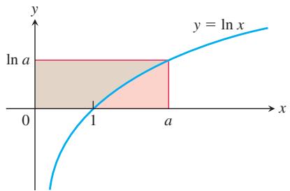
Show that for any number $𝑎 > 1$

\int 𝑎 1 l n 𝑥 𝑑 𝑥 + \int l n 𝑎 0 𝑒 𝑦 𝑑 𝑦 = 𝑎 l n 𝑎,

as suggested by the accompanying figure.

教材插图

The geometric, logarithmic, and arithmetic mean inequality

a. Show that the graph of $𝑒 𝑥$ is concave up over every interval of x-values.

b. Show, by reference to the accompanying figure, that if

$0 < 𝑎 < 𝑏$ , then

𝑒 (l n 𝑎 + l n 𝑏) / 2 \cdot (l n 𝑏 - l n 𝑎) < \int l n 𝑏 l n 𝑎 𝑒 𝑥 𝑑 𝑥 < 𝑒 l n 𝑎 + 𝑒 l n 𝑏 2 \cdot (l n 𝑏 - l n 𝑎) .

教材插图

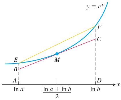
NOT TO SCALE

c. Use the inequality in part (b) to conclude that

\sqrt 𝑎 𝑏 < 𝑏 - 𝑎 l n 𝑏 - l n 𝑎 < 𝑎 + 𝑏 2 .

This inequality says that the geometric mean of two positive numbers is less than their logarithmic mean, which in turn is less than their arithmetic mean.

Use Figure 7.1 and appropriate areas to show that

12 + 13 + 14 + \dots + 1 𝑛 < l n 𝑛 < 1 + 12 + 13 + \dots + 1 𝑛 - 1 . 62 . $ 𝑃 𝑎 𝑟 𝑡 𝑖 𝑡 𝑖 𝑜 𝑛 𝑡 ℎ 𝑒 𝑖 𝑛 𝑡 𝑒 𝑟 𝑣 𝑎 𝑙 $ [1, 2] $ 𝑖 𝑛 𝑡 𝑜 𝑛 𝑒 𝑞 𝑢 𝑎 𝑙 𝑝 𝑎 𝑟 𝑡 𝑠 . 𝑇 ℎ 𝑒 𝑛 𝑢 𝑠 𝑒 𝐹 𝑖 𝑔 𝑢 𝑟 𝑒 7.1 𝑎 𝑛 𝑑 𝑎 𝑝 𝑝 𝑟 𝑜 𝑝 𝑟 𝑖 𝑎 𝑡 𝑒 𝑝 𝑎 𝑟 𝑡 𝑖 𝑡 𝑖 𝑜 𝑛 𝑝 𝑜 𝑖 𝑛 𝑡 𝑠 𝑎 𝑛 𝑑 𝑎 𝑟 𝑒 𝑎 𝑠 𝑡 𝑜 𝑠 ℎ 𝑜 𝑤 𝑡 ℎ 𝑎 𝑡 $ 1 𝑛 + 1 + 1 𝑛 + 2 + 1 𝑛 + 3 + \dots + 1 2 𝑛 < l n 2 < 1 𝑛 + 1 𝑛 + 1 + 1 𝑛 + 2 + \dots + 1 2 𝑛 - 1 .

Use the same-derivative argument, as was done to prove the Product and Power Rules for logarithms, to prove the Quotient Rule property.
Use the same-derivative argument to prove the identities

𝐚 . t a n - 1 𝑥 + c o t - 1 𝑥 = 𝜋 2 𝐛 . s e c - 1 𝑥 + c s c - 1 𝑥 = 𝜋 2

Starting with the equation $𝑒 𝑥 𝑒 𝑦 = 𝑒 𝑥 + 𝑦$ , derived in the text, show that $𝑒 - 𝑥 = 1 / 𝑒 𝑥$ for any real number $𝑥$ . Then show that $𝑒 𝑥 / 𝑒 𝑦 = 𝑒 𝑥 - 𝑦$ for any numbers $𝑥$ and $𝑦$ .
Show that $(𝑒 𝑥) 𝑦 = 𝑒 𝑥 𝑦 = (𝑒 𝑦) 𝑥$ for any numbers x and y.
Show that properties (2), (3), and (4) of Theorem 2 follow from Theorem 1 and the inverse relationship between the logarithmic and exponential functions.
Alternative proof that $l i m 𝑥 \to \infty (1 + 1 𝑥) 𝑥 = 𝑒$ :

a. Let $𝑥 > 0$ be given, and use Figure 7.1 to show that

1 𝑥 + 1 < \int 𝑥 + 1 𝑥 1 𝑡 𝑑 𝑡 < 1 𝑥 .

b. Conclude from part (a) that

1 𝑥 + 1 < l n (1 + 1 𝑥) < 1 𝑥 .

c. Conclude from part (b) that

𝑒 𝑥 𝑥 + 1 < (1 + 1 𝑥) 𝑥 < 𝑒 .

d. Conclude from part (c) that

l i m 𝑥 \to \infty (1 + 1 𝑥) 𝑥 = 𝑒 .

Grapher Explorations

When solving Exercises 69–76, you may need to use appropriate technology (such as a graphing calculator or a computer).

Graph $l n 𝑥$ , $l n 2 𝑥$ , $l n 4 𝑥$ , $l n 8 𝑥$ , and $l n 16 𝑥$ (as many as you can) together for $0 < 𝑥 \leq 10$ . What is going on? Explain.
Graph $𝑦 = l n | s i n 𝑥 |$ in the window $0 \leq 𝑥 \leq 22, - 2 \leq 𝑦 \leq 0$ . Explain what you see. How could you change the formula to turn the arches upside down?
a. Graph $𝑦 = s i n 𝑥$ and the curves $𝑦 = l n (𝑎 + s i n 𝑥)$ for a = 2, 4, 8, 20, and 50 together for $0 \leq 𝑥 \leq 23$ .

b. Why do the curves flatten as $𝑎$ increases? (Hint: Find an $𝑎$ -dependent upper bound for $| 𝑦' |$ .)

Does the graph of $𝑦 = \sqrt 𝑥 - l n 𝑥, 𝑥 > 0$ , have an inflection point? Try to answer the question (a) by graphing, (b) by using calculus.
The equation $𝑥 2 = 2 𝑥$ has three solutions: $𝑥 = 2, 𝑥 = 4$ , and one other. Estimate the third solution as accurately as you can by graphing.
Could $𝑥 l n 2$ possibly be the same as $2 l n 𝑥$ for some x > 0? Graph the two functions and explain what you see.
Which is bigger, $𝜋 𝑒$ or $𝑒 𝜋$ ? Calculators have taken some of the mystery out of this once-challenging question. (Go ahead and check; you will see that it is a surprisingly close call.) You can answer the question without a calculator, though.

a. Find an equation for the line through the origin tangent to the graph of $𝑦 = l n 𝑥$ .

教材插图

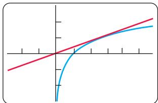
[-3, 6] by [-3, 3]

b. Give an argument based on the graphs of $𝑦 = l n 𝑥$ and the tangent line to explain why $l n 𝑥 < 𝑥 / 𝑒$ for all positive $𝑥 \neq 𝑒$ .

c. Show that $l n (𝑥 𝑒) < 𝑥$ for all positive $𝑥 \neq 𝑒$ .

d. Conclude that $𝑥 𝑒 < 𝑒 𝑥$ for all positive $𝑥 \neq 𝑒$ .

e. So which is bigger, $𝜋 𝑒$ or $𝑒 𝜋$ ?

A decimal representation of $𝑒$ Find $𝑒$ to as many decimal places as you can by solving the equation $l n 𝑥 = 1$ using Newton’s method in Section 4.7.

Calculations with Other Bases

Most scientific calculators have keys for $l o g 10 𝑥$ and $l n 𝑥$ . To find logarithms to other bases, we use the equation $l o g 𝑎 𝑥 = (l n 𝑥) / (l n 𝑎)$ .

Find the following logarithms to five decimal places.

a. $l o g 3 8$

b. $l o g 7 0.5$

c. $l o g 20 17$

d. $l o g 0.5 7$

e. $l n 𝑥$ , given that $l o g 10 𝑥 = 2.3$

f. $l n 𝑥$ , given that $l o g 2 𝑥 = 1.4$

g. $l n 𝑥$ , given that $l o g 2 𝑥 = - 1.5$

h. $l n 𝑥$ , given that $l o g 10 𝑥 = - 0.7$

Conversion factors

a. Show that the equation for converting base 10 logarithms to base 2 logarithms is

l o g 2 𝑥 = l n 10 l n 2 l o g 10 𝑥 .

b. Show that the equation for converting base $𝑎$ logarithms to base $𝑏$ logarithms is

l o g 𝑏 𝑥 = l n 𝑎 l n 𝑏 l o g 𝑎 𝑥 .

7.2 Exponential Change and Separable Differential Equations

Exponential functions increase or decrease very rapidly with changes in the independent variable. They describe growth or decay in many natural and industrial situations. The variety of models based on these functions partly accounts for their importance.

Exponential Change

In modeling many real-world situations, a quantity y increases or decreases at a rate proportional to its size at a given time t. Examples of such quantities include the size of a population, the amount of a decaying radioactive material, and the temperature difference between a hot object and its surrounding medium. Such quantities are said to undergo exponential change.

教材插图

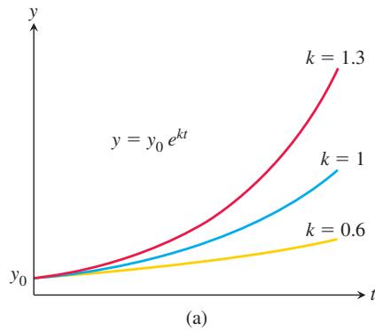
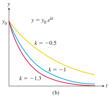
FIGURE 7.5 Graphs of (a) exponential growth and (b) exponential decay. As $| 𝑘 |$ increases, the growth $(𝑘 > 0)$ or decay $(𝑘 < 0)$ intensifies.

If the amount present at time t = 0 is called $𝑦 0$ , then we can find y as a function of t by solving the following initial value problem:

D i f f e r e n t i a l e q u a t i o n : 𝑑 𝑦 𝑑 𝑡 = 𝑘 𝑦 (1 a)

I n i t i a l c o n d i t i o n : 𝑦 = 𝑦 0 w h e n 𝑡 = 0 . (1 b)

If y is positive and increasing, then k is positive, and we use Equation (1a) to say that the rate of growth is proportional to what has already been accumulated. If y is positive and decreasing, then k is negative, and we use Equation (1a) to say that the rate of decay is proportional to the amount still left.

The constant function $𝑦 = 0$ is a solution of Equation (1a) if $𝑦 0 = 0$ . To find the solutions when $𝑦 0$ is not zero, we divide Equation (1a) by $𝑦$ :

1 𝑦 \cdot 𝑑 𝑦 𝑑 𝑡 = 𝑘 𝑦 \neq 0 \int 1 𝑦 𝑑 𝑦 𝑑 𝑡 𝑑 𝑡 = \int 𝑘 𝑑 𝑡 I n t e g r a t e w i t h r e s p e c t t o 𝑡 . l n | 𝑦 | = 𝑘 𝑡 + 𝐶 \int (1 / 𝑢) 𝑑 𝑢 = l n | 𝑢 | + 𝐶 | 𝑦 | = 𝑒 𝑘 𝑡 + 𝐶 E x p o n e n t i a t e . | 𝑦 | = 𝑒 𝐶 \cdot 𝑒 𝑘 𝑡 𝑒 𝑎 + 𝑏 = 𝑒 𝑎 \cdot 𝑒 𝑏 𝑦 = \pm 𝑒 𝐶 𝑒 𝑘 𝑡 I f | 𝑦 | = 𝑟, t h e n 𝑦 = \pm 𝑟 . 𝑦 = 𝐴 𝑒 𝑘 𝑡 . 𝐴 i s a s h o r t e r n a m e f o r \pm 𝑒 𝐶 .

By allowing $𝐴$ to take on the value 0 in addition to all possible values $\pm 𝑒 𝐶$ , we can include the solution $𝑦 = 0$ (which occurs when $𝑦 0 = 0$ ) in the formula.

We find the value of A for the initial value problem by solving for A when $𝑦 = 𝑦 0$ and t = 0:

𝑦 0 = 𝐴 𝑒 𝑘 \cdot 0 = 𝐴 .

The solution of the initial value problem

𝑑 𝑦 𝑑 𝑡 = 𝑘 𝑦, 𝑦 (0) = 𝑦 0

𝑦 = 𝑦 0 𝑒 𝑘 𝑡 . (2)

Quantities changing in this way are said to undergo exponential growth if k > 0 and exponential decay if k < 0. The number k is called the rate constant of the change. (See Figure 7.5.)

The derivation of Equation (2) shows also that the only functions that are their own derivatives $(𝑘 = 1)$ are constant multiples of the exponential function.

Before presenting several examples of exponential change, let us consider the process we used to derive it.

Separable Differential Equations

Exponential change is modeled by a differential equation of the form dy/dx = ky, where k is a nonzero constant. More generally, suppose we have a differential equation of the form

𝑑 𝑦 𝑑 𝑥 = 𝑓 (𝑥, 𝑦), (3)

where f is a function of both the independent and dependent variables. A solution of the equation is a differentiable function $𝑦 = 𝑦 (𝑥)$ defined on an interval of x-values (perhaps infinite) such that

𝑑 𝑑 𝑥 𝑦 (𝑥) = 𝑓 (𝑥, 𝑦 (𝑥))

on that interval. That is, when $𝑦 (𝑥)$ and its derivative $𝑦' (𝑥)$ are substituted into the differential equation, the resulting equation is true for all x in the solution interval. The general solution is a solution $𝑦 (𝑥)$ that contains all possible solutions, and it always contains an arbitrary constant.

Equation (3) is separable if $𝑓$ can be expressed as a product of a function of $𝑥$ and a function of $𝑦$ . The differential equation then has the form

𝑑 𝑦 𝑑 𝑥 = 𝑔 (𝑥) 𝐻 (𝑦) . 𝑔 i s a f u n c t i o n o f 𝑥; 𝐻 i s a f u n c t i o n o f 𝑦 .

Then collect all of the y factors so that they are together with dy, and likewise collect all of the x factors together with dx:

1 𝐻 (𝑦) 𝑑 𝑦 = 𝑔 (𝑥) 𝑑 𝑥 .

Now we integrate both sides of this equation:

\int 1 𝐻 (𝑦) 𝑑 𝑦 = \int 𝑔 (𝑥) 𝑑 𝑥 . (4)

After completing the integrations, we obtain the solution y, defined implicitly as a function of x.

The justification that we can integrate both sides in Equation (4) in this way is based on the Substitution Rule (Section 5.5):

\int 1 𝐻 (𝑦) 𝑑 𝑦 = \int 1 𝐻 (𝑦 (𝑥)) 𝑑 𝑦 𝑑 𝑥 𝑑 𝑥 = \int 1 𝐻 (𝑦 (𝑥)) 𝐻 (𝑦 (𝑥)) 𝑔 (𝑥) 𝑑 𝑥 𝑑 𝑦 𝑑 𝑥 = 𝐻 (𝑦 (𝑥)) 𝑔 (𝑥) = \int 𝑔 (𝑥) 𝑑 𝑥 .

EXAMPLE 1 Solve the differential equation

𝑑 𝑦 𝑑 𝑥 = (1 + 𝑦) 𝑒 𝑥, 𝑦 > - 1 .

Solution Since $1 + 𝑦$ is never zero for y > -1, we can solve the equation by separating the variables.

𝑑 𝑦 𝑑 𝑥 = (1 + 𝑦) 𝑒 𝑥

𝑑 𝑦 = (1 + 𝑦) 𝑒 𝑥 𝑑 𝑥

Treat dy/dx as a quotient of differentials and multiply both sides by dx.

𝑑 𝑦 1 + 𝑦 = 𝑒 𝑥 𝑑 𝑥

D i v i d e b y (1 + 𝑦) .

\int 𝑑 𝑦 1 + 𝑦 = \int 𝑒 𝑥 𝑑 𝑥

Integrate both sides.

l n (1 + 𝑦) = 𝑒 𝑥 + 𝐶

C represents the combined constants

of integration.

The last equation gives y as an implicit function of x.

EXAMPLE 2 Solve the equation $𝑦 (𝑥 + 1) 𝑑 𝑦 𝑑 𝑥 = 𝑥 (𝑦 2 + 1)$ .

Solution We change to differential form, separate the variables, and integrate:

𝑦 (𝑥 + 1) 𝑑 𝑦 = 𝑥 (𝑦 2 + 1) 𝑑 𝑥

𝑦 𝑑 𝑦 𝑦 2 + 1 = 𝑥 𝑑 𝑥 𝑥 + 1

\int 𝑦 𝑑 𝑦 1 + 𝑦 2 = \int (1 - 1 𝑥 + 1) 𝑑 𝑥 D i v i d e 𝑥 b y 𝑥 + 1 .

12 l n (1 + 𝑦 2) = 𝑥 - l n | 𝑥 + 1 | + 𝐶 .

The last equation gives the solution y as an implicit function of x.

教材插图

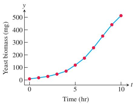
FIGURE 7.6 Graph of the growth of a yeast population over a 10-hour period, based on the data in Table 7.3.

TABLE 7.3 Population of yeast

The initial value problem

Time (hr)	Yeast biomass (mg)
0	9.6
1	18.3
2	29.0
3	47.2
4	71.1
5	119.1
6	174.6
7	257.3
8	350.7
9	441.0
10	513.3

𝑑 𝑦 𝑑 𝑡 = 𝑘 𝑦, 𝑦 (0) = 𝑦 0

involves a separable differential equation, and the solution $𝑦 = 𝑦 0 𝑒 𝑘 𝑡$ expresses exponential change. We now present several examples of such change.

Unlimited Population Growth

Strictly speaking, the number of individuals in a population (of people, plants, animals, or bacteria, for example) is a discontinuous function of time because it takes on discrete values. However, when the number of individuals becomes large enough, the population can be approximated by a continuous function. Differentiability of the approximating function is another reasonable hypothesis in many settings, allowing for the use of calculus to model and predict population sizes.

If we assume that the proportion of reproducing individuals remains constant and assume a constant fertility, then at any instant t the birth rate is proportional to the number $𝑦 (𝑡)$ of individuals present. We likewise assume that the death rate of the population is stable and proportional to $𝑦 (𝑡)$ . If, further, we neglect departures and arrivals, the growth rate dy/dt is the birth rate minus the death rate, which is the difference of the two proportionalities under our assumptions. In other words, dy/dt = ky so that $𝑦 = 𝑦 0 𝑒 𝑘 𝑡$ , where $𝑦 0$ is the size of the population at time t = 0. As with all kinds of growth, there may be limitations imposed by the surrounding environment, but we will not go into these here. (We treat one model imposing such limitations in Section 16.4.) When k is positive, the proportionality dy/dt = ky models unlimited population growth. (See Figure 7.6.)

EXAMPLE 3 The biomass of a yeast culture in an experiment is initially 29 grams. After 30 minutes the mass is 37 grams. Assuming that the equation for unlimited population growth gives a good model for the growth of the yeast when the mass is below 100 grams, how long will it take for the mass to double from its initial value?

Solution Let $𝑦 (𝑡)$ be the yeast biomass after t minutes. We use the exponential growth model dy/dt = ky for unlimited population growth, with solution $𝑦 = 𝑦 0 𝑒 𝑘 𝑡$ .

We have $𝑦 0 = 𝑦 (0) = 29$ . We are also told that

𝑦 (30) = 29 𝑒 𝑘 (30) = 3 7 .

Solving this equation for k, we find

𝑒 𝑘 (30) = 3729

30 𝑘 = l n (3729)

𝑘 = 130 l n (3729) \approx 0 . 00811 8 .

Then the mass of the yeast in grams after t minutes is given by the equation

𝑦 = 29 𝑒 (0 . 008118) 𝑡 .

To solve the problem, we find the time t for which $𝑦 (𝑡) = 58$ , which is twice the initial amount.

29 𝑒 (0 . 008118) 𝑡 = 58 (0 . 008118) 𝑡 = l n (5829) 𝑡 = l n 2 0.008118 \approx 8 5 . 38

It takes about 85 minutes for the yeast population to double.

In the next example we model the number of people within a given population who are infected by a disease that is being eradicated from the population. Here the constant of proportionality k is negative, and the model describes an exponentially decaying number of infected individuals.

EXAMPLE 4 One model for the way diseases die out when properly treated assumes that the rate dy/dt at which the number of infected people changes is proportional to the number y. The number of people cured is proportional to the number y that are infected with the disease. Suppose that in the course of any given year, the number of cases of a disease is reduced by 20%. If there are 10,000 cases today, how many years will it take to reduce the number to 1000?

Solution We use the equation $𝑦 = 𝑦 0 𝑒 𝑘 𝑡$ . There are three things to find: the value of $𝑦 0$ , the value of k, and the time t when y = 1000.

The value of $𝑦 0$ . We are free to count time beginning anywhere we want. If we count from today, then y = 10,000 when t = 0, so $𝑦 0 = 10, 000$ . Our equation is now

𝑦 = 10, 000 𝑒 𝑘 𝑡 . (5)

The value of k. When t = 1 year, the number of cases will be 80% of its present value, or 8000. Hence,

8000 = 10, 000 𝑒 𝑘 (1) E q . (5) w i t h 𝑡 = 1 a n d 𝑦 = 8000 𝑒 𝑘 = 0 . 8 l n (𝑒 𝑘) = l n 0 . 8 T a k e l o g s o f b o t h s i d e s 𝑘 = l n 0 . 8 < 0 . l n 0 . 8 \approx - 0 . 223

At any given time t,

𝑦 = 10, 000 𝑒 (l n 0 . 8) 𝑡 . (6)

教材插图

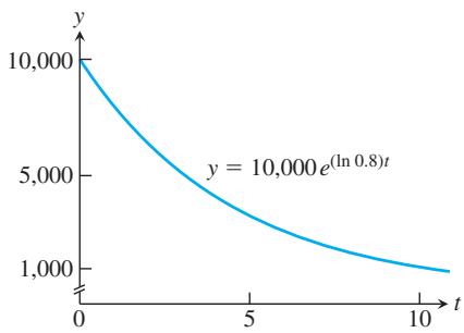
FIGURE 7.7 A graph of the number of people infected by a disease exhibits exponential decay (Example 4).

For radon-222 gas, t is measured in days and k = 0.18. For radium-226, which used to be painted on watch dials to make them glow at night (a dangerous practice), t is measured in years and $𝑘 = 4.3 \times 10 - 4$ .

The value of $𝑡$ that makes $𝑦 = 1000$ . We set $𝑦$ equal to 1000 in Equation (6) and solve for $𝑡$ :

1000 = 10, 000 𝑒 (l n 0 . 8) 𝑡 𝑒 (l n 0 . 8) 𝑡 = 0 . 1 (l n 0 . 8) 𝑡 = l n 0 . 1 𝑡 = l n 0.1 l n 0.8 \approx 1 0 . 32 y e a r s . T a k e l o g s o f b o t h s i d e s

It will take a little more than 10 years to reduce the number of cases to 1000. (See Figure 7.7.)

Radioactivity

Some atoms are unstable and can spontaneously emit mass or radiation. This process is called radioactive decay, and an element whose atoms go spontaneously through this process is called radioactive. Sometimes when an atom emits some of its mass through this process of radioactivity, the remainder of the atom re-forms to make an atom of some new element. For example, radioactive carbon-14 decays into nitrogen; radium, through a number of intermediate radioactive steps, decays into lead.

Experiments have shown that at any given time, the rate at which a radioactive element decays (as measured by the number of nuclei that change per unit time) is approximately proportional to the number of radioactive nuclei present. Thus, the decay of a radioactive element is described by the equation $𝑑 𝑦 / 𝑑 𝑡 = - 𝑘 𝑦$ , k > 0. It is conventional to use -k, with k > 0, to emphasize that y is decreasing. If $𝑦 0$ is the number of radioactive nuclei present at time zero, the number still present at any later time t will be

𝑦 = 𝑦 0 𝑒 - 𝑘 𝑡, 𝑘 > 0 .

In Section 1.5, we defined the half-life of a radioactive element to be the time required for half of the radioactive nuclei present in a sample to decay. It is an interesting fact that the half-life is a constant that does not depend on the number of radioactive nuclei initially present in the sample, but only on the radioactive substance. We found that the half-life is given by the following equation.

H a l f - l i f e = l n 2 𝑘 (7)

For example, the half-life for radon-222 is

h a l f - l i f e = l n 2 0.18 \approx 3 . 9 d a y s .

Carbon-14 dating uses the half-life of 5730 years.

EXAMPLE 5 The decay of radioactive elements can sometimes be used to date events from Earth’s past. In a living organism, the ratio of radioactive carbon, carbon-14, to ordinary carbon stays fairly constant during the lifetime of the organism, being approximately equal to the ratio in the organism’s atmosphere at the time. After the organism’s death, however, no new carbon is ingested, and the proportion of carbon-14 in the organism’s remains decreases as the carbon-14 decays.

Scientists who do carbon-14 dating often use a figure of 5730 years for its half-life. Find the age of a sample in which 10% of the radioactive nuclei originally present have decayed.

Solution We use the decay equation $𝑦 = 𝑦 0 𝑒 - 𝑘 𝑡$ . There are two things to find: the value of k and the value of t when y is $0.9 𝑦 0$ (90% of the radioactive nuclei are still present). That is, find t when $𝑦 0 𝑒 - 𝑘 𝑡 = 0.9 𝑦 0$ , or $𝑒 - 𝑘 𝑡 = 0.9$ .

The value of k. We use the half-life Equation (7):

𝑘 = l n 2 h a l f - l i f e = l n 2 5730 (a b o u t 1 . 2 \times 1 0 - 4) .

The value of $𝑡$ that makes $𝑒 - 𝑘 𝑡 = 0.9$ .

𝑒 - 𝑘 𝑡 = 0 . 9 𝑒 - (l n 2 / 5730) 𝑡 = 0 . 9 - l n 2 5730 𝑡 = l n 0 . 9 𝑡 = - 5730 l n 0.9 l n 2 \approx 871 y e a r s T a k e l o g s o f b o t h s i d e s

The sample is about 871 years old.

Heat Transfer: Newton’s Law of Cooling

Hot soup left in a tin cup cools to the temperature of the surrounding air. A hot silver bar immersed in a large tub of water cools to the temperature of the surrounding water. In situations like these, the rate at which an object’s temperature is changing at any given time is roughly proportional to the difference between its temperature and the temperature of the surrounding medium. This observation is called Newton’s Law of Cooling, although it applies to warming as well.

If H is the temperature of the object at time t, and $𝐻 𝑆$ is the constant surrounding temperature, then the differential equation is

𝑑 𝐻 𝑑 𝑡 = - 𝑘 (𝐻 - 𝐻 𝑆) . (8)

If we substitute $𝑦$ for $(𝐻 - 𝐻 𝑆)$ , then

𝑑 𝑦 𝑑 𝑡 = 𝑑 𝑑 𝑡 (𝐻 - 𝐻 𝑆) = 𝑑 𝐻 𝑑 𝑡 - 𝑑 𝑑 𝑡 (𝐻 𝑆) = 𝑑 𝐻 𝑑 𝑡 - 0 = 𝑑 𝐻 𝑑 𝑡 = - 𝑘 (𝐻 - 𝐻 𝑆) = - 𝑘 𝑦 . E q . (8) 𝐻 - 𝐻 𝑆 = 𝑦

We know that the solution of the equation $𝑑 𝑦 / 𝑑 𝑡 = - 𝑘 𝑦$ is $𝑦 = 𝑦 0 𝑒 - 𝑘 𝑡$ , where $𝑦 (0) = 𝑦 0$ . Substituting $(𝐻 - 𝐻 𝑆)$ for $𝑦$ , this says that

𝐻 - 𝐻 𝑆 = (𝐻 0 - 𝐻 𝑆) 𝑒 - 𝑘 𝑡, (9)

where $𝐻 0$ is the temperature at $𝑡 = 0$ . This equation is the solution to Newton’s Law of Cooling.

EXAMPLE 6 A hard-boiled egg at $98 \circ C$ is put in a sink of $18 \circ C$ water. After 5 min, the egg’s temperature is $38 \circ C$ . Assuming that the water has not warmed appreciably, how much longer will it take the egg to reach $20 \circ C$ ?

Solution We find how long it would take the egg to cool from $98 \circ C$ to $20 \circ C$ and subtract the 5 min that have already elapsed. Using Equation (9) with $𝐻 𝑆 = 18$ and $𝐻 0 = 98$ , the egg’s temperature $𝑡$ min after it is put in the sink is

𝐻 = 18 + (98 - 18) 𝑒 - 𝑘 𝑡 = 18 + 80 𝑒 - 𝑘 𝑡 .

To find k, we use the information that H = 38 when t = 5:

38 = 18 + 80 𝑒 - 5 𝑘

𝑒 - 5 𝑘 = 14

- 5 𝑘 = l n 14 = - l n 4

𝑘 = 15 l n 4 = 0 . 2 l n 4 (a b o u t 0 . 28) .

The egg’s temperature at time $𝑡$ is $𝐻 = 18 + 80 𝑒 - (0.2 l n 4) 𝑡$ . Now find the time $𝑡$ when $𝐻 = 20$ :

20 = 18 + 80 𝑒 - (0 . 2 l n 4) 𝑡

80 𝑒 - (0 . 2 l n 4) 𝑡 = 2

𝑒 - (0 . 2 l n 4) 𝑡 = 140

- (0 . 2 l n 4) 𝑡 = l n 140 = - l n 40

𝑡 = l n 40 0.2 l n 4 \approx 13 m i n .

The egg’s temperature will reach $20 \circ C$ about 13 min after it is put in the water to cool. Since it took 5 min to reach $38 \circ C$ , it will take about 8 min more to reach $20 \circ C$ .

EXERCISES

Verifying Solutions

In Exercises 1–4, show that each function $𝑦 = 𝑓 (𝑥)$ is a solution of the accompanying differential equation.

$2 𝑦' + 3 𝑦 = 𝑒 - 𝑥$

a. $𝑦 = 𝑒 - 𝑥$

𝐛 . 𝑦 = 𝑒 - 𝑥 + 𝑒 - (3 / 2) 𝑥

c. $𝑦 = 𝑒 - 𝑥 + 𝐶 𝑒 - (3 / 2) 𝑥$

$𝑦' = 𝑦 2$

a. $𝑦 = - 1 𝑥$ b. $𝑦 = - 1 𝑥 + 3$ c. $𝑦 = - 1 𝑥 + 𝐶$

$𝑦 = 1 𝑥 \int 𝑥 1 𝑒 𝑡 𝑡 𝑑 𝑡, 𝑥 2 𝑦' + 𝑥 𝑦 = 𝑒 𝑥$

𝑦 = 1 \sqrt 1 + 𝑥 4 \int 𝑥 1 \sqrt 1 + 𝑡 4 𝑑 𝑡, 𝑦' + 2 𝑥 3 1 + 𝑥 4 𝑦 = 1

Initial Value Problems

In Exercises 5–8, show that each function is a solution of the given initial value problem.

Differential equation	Initial equation	Solution candidate
5. $𝑦' + 𝑦 = 2 1 + 4 𝑒 2 𝑥$	$𝑦 (- l n 2) = 𝜋 2$	$𝑦 = 𝑒 - 𝑥 t a n - 1 (2 𝑒 𝑥)$
6. $𝑦' = 𝑒 - 𝑥 2 - 2 𝑥 𝑦$	$𝑦 (2) = 0$	$𝑦 = (𝑥 - 2) 𝑒 - 𝑥 2$
7. $𝑥 𝑦' + 𝑦 = - s i n 𝑥,$ $𝑥 > 0$	$𝑦 (𝜋 2) = 0$	$𝑦 = c o s 𝑥 𝑥$
8. $𝑥 2 𝑦' = 𝑥 𝑦 - 𝑦 2,$ $𝑥 > 1$	$𝑦 (𝑒) = 𝑒$	$𝑦 = 𝑥 l n 𝑥$

Solve the differential equation in Exercises 9–22.

Separable Differential Equations

$2 \sqrt 𝑥 𝑦 𝑑 𝑦 𝑑 𝑥 = 1, 𝑥, 𝑦 > 0$
$𝑑 𝑦 𝑑 𝑥 = 𝑥 2 \sqrt 𝑦, 𝑦 > 0$
$𝑑 𝑦 𝑑 𝑥 = 𝑒 𝑥 - 𝑦$
$𝑑 𝑦 𝑑 𝑥 = 3 𝑥 2 𝑒 - 𝑦$
$𝑑 𝑦 𝑑 𝑥 = \sqrt 𝑦 c o s 2 \sqrt 𝑦$
$\sqrt 2 𝑥 𝑦 𝑑 𝑦 𝑑 𝑥 = 1$
$\sqrt 𝑥 𝑑 𝑦 𝑑 𝑥 = 𝑒 𝑦 + \sqrt 𝑥, 𝑥 > 0$ 16. (sec $𝑥$ ) $𝑑 𝑦 𝑑 𝑥 = 𝑒 𝑦 + s i n 𝑥$
$𝑑 𝑦 𝑑 𝑥 = 2 𝑥 \sqrt 1 - 𝑦 2, - 1 < 𝑦 < 1$
$𝑑 𝑦 𝑑 𝑥 = 𝑒 2 𝑥 - 𝑦 𝑒 𝑥 + 𝑦$
$𝑦 2 𝑑 𝑦 𝑑 𝑥 = 3 𝑥 2 𝑦 3 - 6 𝑥 2$
$𝑑 𝑦 𝑑 𝑥 = 𝑥 𝑦 + 3 𝑥 - 2 𝑦 - 6$
$1 𝑥 𝑑 𝑦 𝑑 𝑥 = 𝑦 𝑒 𝑥 2 + 2 \sqrt 𝑦 𝑒 𝑥 2$
$𝑑 𝑦 𝑑 𝑥 = 𝑒 𝑥 - 𝑦 + 𝑒 𝑥 + 𝑒 - 𝑦 + 1$

Applications and Examples

The answers to most of the following exercises are in terms of logarithms and exponentials. A calculator can be helpful, enabling you to express the answers in decimal form.

Human evolution continues The analysis of tooth shrinkage by C. Loring Brace and colleagues at the University of Michigan’s

Museum of Anthropology indicates that human tooth size is continuing to decrease and that the evolutionary process has not yet come to a halt. In northern Europeans, for example, tooth size reduction now has a rate of 1% per 1000 years.

a. If t represents time in years and y represents tooth size, use the condition that $𝑦 = 0.99 𝑦 0$ when t = 1000 to find the value of k in the equation $𝑦 = 𝑦 0 𝑒 𝑘 𝑡$ . Then use this value of k to answer the following questions.

b. In about how many years will human teeth be 90% of their present size?

c. What will be our descendants’ tooth size 20,000 years from now (as a percentage of our present tooth size)?

Atmospheric pressure The earth’s atmospheric pressure $𝑝$ is often modeled by assuming that the rate $𝑑 𝑝 / 𝑑 ℎ$ at which $𝑝$ changes with the altitude $ℎ$ above sea level is proportional to $𝑝$ . Suppose that the pressure at sea level is 1013 hectopascals and that the pressure at an altitude of $20 k m$ is 90 hectopascals.

a. Solve the initial value problem

D i f f e r e n t i a l e q u a t i o n : 𝑑 𝑝 / 𝑑 ℎ = 𝑘 𝑝 (𝑘 a c o n s t a n t) I n i t i a l c o n d i t i o n : 𝑝 = 𝑝 0 w h e n ℎ = 0

to express p in terms of h. Determine the values of $𝑝 0$ and k from the given altitude-pressure data.

b. What is the atmospheric pressure at h = 50 km?

c. At what altitude does the pressure equal 900 hectopascals?

First-order chemical reactions In some chemical reactions, the rate at which the amount of a substance changes with time is proportional to the amount present. For the change of $𝛿$ -gluconolactone into gluconic acid, for example,

𝑑 𝑦 𝑑 𝑡 = - 0 . 6 𝑦

when t is measured in hours. If there are 100 grams of $𝛿$ -gluconolactone present when t = 0, how many grams will be left after the first hour?

The inversion of sugar The processing of raw sugar has a step called “inversion” that changes the sugar’s molecular structure. Once the process has begun, the rate of change of the amount of raw sugar is proportional to the amount of raw sugar remaining. If 1000 kg of raw sugar reduces to 800 kg of raw sugar during the first 10 hours, how much raw sugar will remain after another 14 hours?
Working underwater The intensity $𝐿 (𝑥)$ of light x meters beneath the surface of the ocean satisfies the differential equation

𝑑 𝐿 𝑑 𝑥 = - 𝑘 𝐿 .

As a diver, you know from experience that diving to 6 m in the Caribbean Sea cuts the intensity in half. You cannot work without artificial light when the intensity falls below one-tenth of the surface value. About how deep can you expect to work without artificial light?

Voltage in a discharging capacitor Suppose that electricity is draining from a capacitor at a rate that is proportional to the voltage V across its terminals and that, if t is measured in seconds,

𝑑 𝑉 𝑑 𝑡 = - 140 𝑉 .

Solve this equation for V, using $𝑉 0$ to denote the value of V when t = 0. How long will it take the voltage to drop to 10% of its original value?

Cholera bacteria Suppose that the bacteria in a colony can grow unchecked, by the law of exponential change. The colony starts with 1 bacterium and doubles every half-hour. How many bacteria will the colony contain at the end of 24 hours? (Under favorable laboratory conditions, the number of cholera bacteria can double every 30 min. In an infected person, many bacteria are destroyed, but this example helps explain why a person who feels well in the morning may be dangerously ill by evening.)
Growth of bacteria A colony of bacteria is grown under ideal conditions in a laboratory so that the population increases exponentially with time. At the end of 3 hours there are 10,000 bacteria. At the end of 5 hours there are 40,000. How many bacteria were present initially?
The incidence of a disease (Continuation of Example 4.) Suppose that in any given year the number of cases can be reduced by 25% instead of 20%.

a. How long will it take to reduce the number of cases to 1000?

b. How long will it take to eradicate the disease—that is, reduce the number of cases to less than 1?

Drug concentration An antibiotic is administered intravenously into the bloodstream at a constant rate $𝑟$ . As the drug flows through the patient’s system and acts on the infection that is present, it is removed from the bloodstream at a rate proportional to the amount in the bloodstream at that time. Since the amount of blood in the patient is constant, this means that the concentration $𝑦 = 𝑦 (𝑡)$ of the antibiotic in the bloodstream can be modeled by the differential equation

𝑑 𝑦 𝑑 𝑡 = 𝑟 - 𝑘 𝑦, 𝑘 > 0 a n d c o n s t a n t .

a. If $𝑦 (0) = 𝑦 0$ , find the concentration $𝑦 (𝑡)$ at any time t.

b. Assume that $𝑦 0 < (𝑟 / 𝑘)$ and find $l i m 𝑦 \to \infty 𝑦 (𝑡)$ . Sketch the solution curve for the concentration.

Endangered species Biologists consider a species of animal or plant to be endangered if it is expected to become extinct within 20 years. If a certain species of wildlife is counted to have 1147 members at the present time, and the population has been steadily declining exponentially at an annual rate averaging 39% over the past 7 years, do you think the species is endangered? Explain your answer.
The U.S. population The U.S. Census Bureau keeps a running clock totaling the U.S. population. On April 19, 2021, the total was increasing at the rate of 1 person every 40 s. The population figure for 1
p.m. EST on that day was 330,215,841.

a. Assuming exponential growth at a constant rate, find the rate constant for the population’s growth (people per 365-day year).

b. At this rate, what will the U.S. population be at 1

P.M. EST on April 19, 2028?

Oil depletion Suppose the amount of oil pumped from one of the canyon wells in Whittier, California, decreases at the continuous rate of $10 %$ per year. When will the well’s output fall to one-fifth of its present value?
Continuous price discounting To encourage buyers to place 100-unit orders, your firm’s sales department applies a continuous discount that makes the unit price a function $𝑝 (𝑥)$ of the number of units $𝑥$ ordered. The discount decreases the price at the rate of $0.01 𝑝 𝑒 𝑟 𝑢 𝑛 𝑖 𝑡 𝑜 𝑟 𝑑 𝑒 𝑟 𝑒 𝑑 . 𝑇 ℎ 𝑒 𝑝 𝑟 𝑖 𝑐 𝑒 𝑝 𝑒 𝑟 𝑢 𝑛 𝑖 𝑡 𝑓 𝑜 𝑟 𝑎 100 - 𝑢 𝑛 𝑖 𝑡 𝑜 𝑟 𝑑 𝑒 𝑟 𝑖 𝑠$ p(100) = $20.09$ .

a. Find $𝑝 (𝑥)$ by solving the following initial value problem.

Differential equation:

𝑑 𝑝 𝑑 𝑥 = - 1100 𝑝

Initial condition:

𝑝 (100) = 2 0 . 09

b. Find the unit price $𝑝 (10)$ for a 10-unit order and the unit price $𝑝 (90)$ for a 90-unit order.

c. The sales department has asked you to find out if it is discounting so much that the firm’s revenue, $𝑟 (𝑥) = 𝑥 \cdot 𝑝 (𝑥)$ , will actually be less for a 100-unit order than, say, for a 90-unit order. Reassure them by showing that $𝑟$ has its maximum value at $𝑥 = 100$ .

d. Graph the revenue function $𝑟 (𝑥) = 𝑥 𝑝 (𝑥)$ for $0 \leq 𝑥 \leq 200$ .

Plutonium-239 The half-life of the plutonium isotope is 24,360 years. If $10 g$ of plutonium is released into the atmosphere by a nuclear accident, how many years will it take for $80 %$ of the isotope to decay?
Polonium-210 The half-life of polonium is 139 days, but your sample will not be useful to you after 95% of the radioactive nuclei present on the day the sample arrives has disintegrated. For about how many days after the sample arrives will you be able to use the polonium?
The mean life of a radioactive nucleus Physicists using the radioactivity equation $𝑦 = 𝑦 0 𝑒 - 𝑘 𝑡$ call the number 1/k the mean life of a radioactive nucleus. The mean life of a radon nucleus is about 1/0.18 = 5.6 days. The mean life of a carbon-14 nucleus is more than 8000 years. Show that 95% of the radioactive nuclei originally present in a sample will disintegrate within three mean lifetimes, i.e., by time t = 3/k. Thus, the mean life of a nucleus gives a quick way to estimate how long the radioactivity of a sample will last.
Californium-252 What costs $27 million per gram and can be used to treat brain cancer, analyze coal for its sulfur content, and detect explosives in luggage? The answer is californium-252, a radioactive isotope discovered by Glenn Seaborg in 1950. Much less than 1g of it is produced each year. The half-life of the isotope is 2.645 years—long enough for a useful service life and short enough to have a high radioactivity per unit mass. One microgram of the isotope releases 170 million neutrons per minute.

a. What is the value of k in the decay equation for this isotope?

b. What is the isotope’s mean life? (See Exercise 39.)

c. How long will it take $95 %$ of a sample’s radioactive nuclei to disintegrate?

Cooling soup Suppose that a cup of soup cooled from $90 \circ C$ to $60 \circ C$ after 10 min in a room where the temperature was $20 \circ C$ . Use Newton’s Law of Cooling to answer the following questions. a. How much longer would it take the soup to cool to $35 \circ C$ ?

b. Instead of being left to stand in the room, the cup of $90 \circ 𝐶$ soup is put in a freezer where the temperature is $- 15 \circ 𝐶$ . How long will it take the soup to cool from $90 \circ 𝐶$ to $35 \circ 𝐶$ ?

A beam of unknown temperature An aluminum beam was brought from the outside cold into a machine shop where the temperature was held at $18 \circ C$ . After $10 m i n$ , the beam warmed to $2 \circ C$ and after another $10 m i n$ , it was $10 \circ C$ . Use Newton’s Law of Cooling to estimate the beam’s initial temperature.
Surrounding medium of unknown temperature A pan of warm water (46 $\circ$ C) was put in a refrigerator. Ten minutes later, the water’s temperature was 39 $\circ$ C; 10 min after that, it was 33 $\circ$ C. Use Newton’s Law of Cooling to estimate how cold the refrigerator was.
Silver cooling in air The temperature of an ingot of silver is $60 ° 𝐶$ above room temperature right now. Twenty minutes ago, it was $70 ° 𝐶$ above room temperature. How far above room temperature will the silver be

a. 15 min from now?

b. 2 hours from now?

c. When will the silver be $10 \circ$ C above room temperature?

The age of Crater Lake The charcoal from a tree killed in the volcanic eruption that formed Crater Lake in Oregon contained 44.5% of the carbon-14 found in living matter. About how old is Crater Lake?
The sensitivity of carbon-14 dating to measurement To see the effect of a relatively small error in the estimate of the amount of carbon-14 in a sample being dated, consider this hypothetical situation:

a. A bone fragment found in central Illinois in the year 2000 contains 17% of its original carbon-14 content. Estimate the year the animal died.

b. Repeat part (a), assuming 18% instead of 17%.

c. Repeat part (a), assuming 16% instead of 17%.

Carbon-14 The oldest known frozen human mummy, discovered in the Schnalstal glacier of the Italian Alps in 1991 and called Otzi, was found wearing straw shoes and a leather coat with goat fur, and holding a copper ax and stone dagger. It was estimated that Otzi died 5000 years before he was discovered in the melting glacier. How much of the original carbon-14 remained in Otzi at the time of his discovery?
Art forgery A painting attributed to Vermeer (1632–1675), which should contain no more than 96.2% of its original carbon-14, contains 99.5% instead. About how old is the forgery?
Lascaux Cave paintings Prehistoric cave paintings of animals were found in the Lascaux Cave in France in 1940. Scientific analysis revealed that only 15% of the original carbon-14 in the paintings remained. What is an estimate of the age of the paintings?
Incan mummy The frozen remains of a young Incan woman were discovered by archeologist Johan Reinhard on Mt. Ampato in Peru during an expedition in 1995.

a. How much of the original carbon-14 was present if the estimated age of the “Ice Maiden” was 500 years?

b. If a 1% error can occur in the carbon-14 measurement, what is the oldest possible age for the Ice Maiden?

7.3 Hyperbolic Functions

Hyperbolic cosine:

(b)

(d)

(e)

The hyperbolic functions are formed by taking combinations of the two exponential functions $𝑒 𝑥$ and $𝑒 - 𝑥$ . The hyperbolic functions simplify many mathematical expressions and occur frequently in mathematical and engineering applications.

Definitions and Identities

The hyperbolic sine and hyperbolic cosine functions are defined by the equations

s i n h 𝑥 = 𝑒 𝑥 - 𝑒 - 𝑥 2 a n d c o s h 𝑥 = 𝑒 𝑥 + 𝑒 - 𝑥 2 .

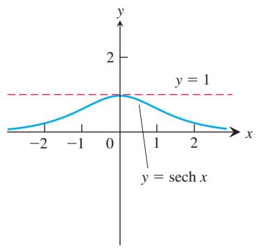
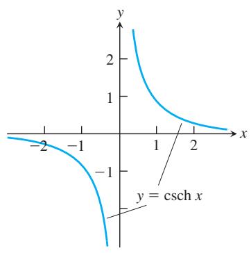
We pronounce sinh x as “cinch x,” rhyming with “pinch x,” and cosh x as “kosh x,” rhyming with “gosh x.” From this basic pair, we define the hyperbolic tangent, cotangent, secant, and cosecant functions. The defining equations and graphs of these functions are shown in Table 7.4. We will see that the hyperbolic functions bear many similarities to the trigonometric functions after which they are named.

TABLE 7.4 The six basic hyperbolic functions

教材插图

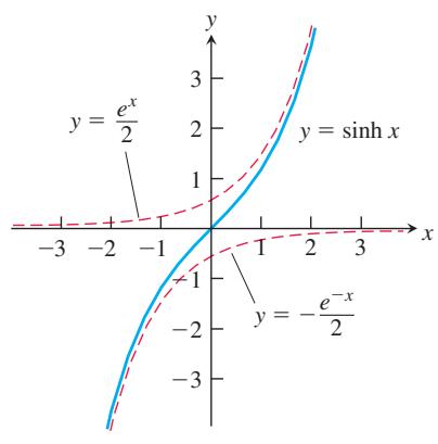
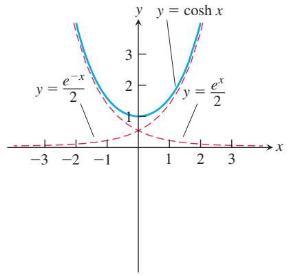
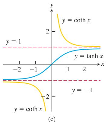
Hyperbolic sine:

Hyperbolic tangent:

$s i n h 𝑥 = 𝑒 𝑥 - 𝑒 - 𝑥 2$

教材插图

t a n h 𝑥 = s i n h 𝑥 c o s h 𝑥 = 𝑒 𝑥 - 𝑒 - 𝑥 𝑒 𝑥 + 𝑒 - 𝑥

𝑥 = 𝑒 𝑥 + 𝑒 - 𝑥 2

教材插图

Hyperbolic cotangent:

Hyperbolic secant:

c o t h 𝑥 = c o s h 𝑥 s i n h 𝑥 = 𝑒 𝑥 + 𝑒 - 𝑥 𝑒 𝑥 - 𝑒 - 𝑥

s e c h 𝑥 = 1 c o s h 𝑥 = 2 𝑒 𝑥 + 𝑒 - 𝑥

Hyperbolic cosecant:

c s c h 𝑥 = 1 s i n h 𝑥 = 2 𝑒 𝑥 - 𝑒 - 𝑥

TABLE 7.5 Identities for hyperbolic functions

c o s h 2 𝑥 - s i n h 2 𝑥 = 1 s i n h 2 𝑥 = 2 s i n h 𝑥 c o s h 𝑥 c o s h 2 𝑥 = c o s h 2 𝑥 + s i n h 2 𝑥 c o s h 2 𝑥 = c o s h 2 𝑥 + 1 2 s i n h 2 𝑥 = c o s h 2 𝑥 - 1 2 t a n h 2 𝑥 = 1 - s e c h 2 𝑥 c o t h 2 𝑥 = 1 + c s c h 2 𝑥

TABLE 7.6 Derivatives of hyperbolic functions

𝑑 𝑑 𝑥 (s i n h 𝑥) = c o s h 𝑥 𝑑 𝑑 𝑥 (c o s h 𝑥) = s i n h 𝑥 𝑑 𝑑 𝑥 (t a n h 𝑥) = s e c h 2 𝑥 𝑑 𝑑 𝑥 (c o t h 𝑥) = - c s c h 2 𝑥 𝑑 𝑑 𝑥 (s e c h 𝑥) = - s e c h 𝑥 t a n h 𝑥 𝑑 𝑑 𝑥 (c s c h 𝑥) = - c s c h 𝑥 c o t h 𝑥

TABLE 7.7 Integral formulas for hyperbolic functions

\int s i n h 𝑥 𝑑 𝑥 = c o s h 𝑥 + 𝐶 \int c o s h 𝑥 𝑑 𝑥 = s i n h 𝑥 + 𝐶 \int s e c h 2 𝑥 𝑑 𝑥 = t a n h 𝑥 + 𝐶 \int c s c h 2 𝑥 𝑑 𝑥 = - c o t h 𝑥 + 𝐶 \int s e c h 𝑥 t a n h 𝑥 𝑑 𝑥 = - s e c h 𝑥 + 𝐶 \int c s c h 𝑥 c o t h 𝑥 𝑑 𝑥 = - c s c h 𝑥 + 𝐶

Hyperbolic functions satisfy the identities in Table 7.5. Except for differences in sign, these resemble identities we know for the trigonometric functions. The identities are proved directly from the definitions, as we show here for the second one:

2 s i n h 𝑥 c o s h 𝑥 = 2 (𝑒 𝑥 - 𝑒 - 𝑥 2) (𝑒 𝑥 + 𝑒 - 𝑥 2) = 𝑒 2 𝑥 - 𝑒 - 2 𝑥 2 S i m p l i f y . = s i n h 2 𝑥 . D e f i n i t i o n o f s i n h

The other identities are obtained similarly, by substituting in the definitions of the hyperbolic functions and using algebra.

For any real number u, we know the point with coordinates $(c o s 𝑢, s i n 𝑢)$ lies on the unit circle $𝑥 2 + 𝑦 2 = 1$ . So the trigonometric functions are sometimes called the circular functions. Because of the first identity

c o s h 2 𝑢 - s i n h 2 𝑢 = 1,

with u substituted for x in Table 7.5, the point having coordinates $(c o s h 𝑢, s i n h 𝑢)$ lies on the right-hand branch of the hyperbola $𝑥 2 - 𝑦 2 = 1$ . This is where the hyperbolic functions get their names (see Exercise 86).

Hyperbolic functions are useful in finding integrals, which we will see in Chapter 8. They play an important role in science and engineering as well. The hyperbolic cosine describes the shape of a hanging cable or wire that is strung between two points at the same height and hanging freely (see Exercise 83). The shape of the St. Louis Arch is an inverted hyperbolic cosine. The hyperbolic tangent occurs in the formula for the velocity of an ocean wave moving over water having a constant depth, and the inverse hyperbolic tangent describes how relative velocities sum according to Einstein’s Law in the Special Theory of Relativity.

Derivatives and Integrals of Hyperbolic Functions

The six hyperbolic functions, being rational combinations of the differentiable functions $𝑒 𝑥$ and $𝑒 - 𝑥$ , have derivatives at every point at which they are defined (Table 7.6). Again, there are similarities to trigonometric functions.

The derivative formulas are obtained from the derivative of $𝑒 𝑥$ :

𝑑 𝑑 𝑥 (s i n h 𝑥) = 𝑑 𝑑 𝑥 (𝑒 𝑥 - 𝑒 - 𝑥 2) D e f i n i t i o n o f s i n h 𝑥 = 𝑒 𝑥 + 𝑒 - 𝑥 2 D e r i v a t i v e o f 𝑒 𝑥 = c o s h 𝑥 . D e f i n i t i o n o f c o s h 𝑥

This gives the first derivative formula. From the definition, we can calculate the derivative of the hyperbolic cosecant function, as follows:

𝑑 𝑑 𝑥 (c s c h 𝑥) = 𝑑 𝑑 𝑥 (1 s i n h 𝑥) D e f i n i t i o n o f c s c h 𝑥 = - c o s h 𝑥 s i n h 2 𝑥 Q u o t i e n t R u l e f o r d e r i v a t i v e s = - 1 s i n h 𝑥 c o s h 𝑥 s i n h 𝑥 R e a r r a n g e f a c t o r s . = - c s c h 𝑥 c o t h 𝑥 D e f i n i t i o n s o f c s c h 𝑥 a n d c o t h 𝑥

The other formulas in Table 7.6 are obtained similarly.

The derivative formulas lead to the integral formulas in Table 7.7.

EXAMPLE 1 We illustrate the derivative and integral formulas.

(a) 𝑑 𝑑 𝑡 (t a n h \sqrt 1 + 𝑡 2) = s e c h 2 \sqrt 1 + 𝑡 2 \cdot 𝑑 𝑑 𝑡 (\sqrt 1 + 𝑡 2) = 𝑡 \sqrt 1 + 𝑡 2 s e c h 2 \sqrt 1 + 𝑡 2

(b) \int c o t h 5 𝑥 𝑑 𝑥 = \int c o s h 5 𝑥 s i n h 5 𝑥 𝑑 𝑥 = 15 \int 𝑑 𝑢 𝑢 𝑢 = s i n h 5 𝑥, 𝑑 𝑢 = 5 c o s h 5 𝑥 𝑑 𝑥 = 15 l n | 𝑢 | + 𝐶 = 15 l n | s i n h 5 𝑥 | + 𝐶

\int 10 s i n h 2 𝑥 𝑑 𝑥 = \int 10 c o s h 2 𝑥 - 1 2 𝑑 𝑥 = 12 \int 10 (c o s h 2 𝑥 - 1) 𝑑 𝑥 = 12 [s i n h 2 𝑥 2 - 𝑥] 10 = s i n h 2 4 - 12 \approx 0 . 40672 (T a b l e 7.5)

(d) \int l n 2 0 4 𝑒 𝑥 s i n h 𝑥 𝑑 𝑥 = \int l n 2 0 4 𝑒 𝑥 𝑒 𝑥 - 𝑒 - 𝑥 2 𝑑 𝑥 = \int l n 2 0 (2 𝑒 2 𝑥 - 2) 𝑑 𝑥 = [𝑒 2 𝑥 - 2 𝑥] l n 2 0 = (𝑒 2 l n 2 - 2 l n 2) - (1 - 0) = 4 - 2 l n 2 - 1 \approx 1 . 6137

Inverse Hyperbolic Functions

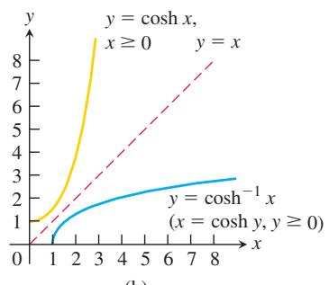
The inverses of the six basic hyperbolic functions are very useful in integration (see Chapter 8). Since $𝑑 (s i n h 𝑥) / 𝑑 𝑥 = c o s h 𝑥 > 0$ , the hyperbolic sine is an increasing function of $𝑥$ . We denote its inverse by

𝑦 = s i n h - 1 𝑥 .

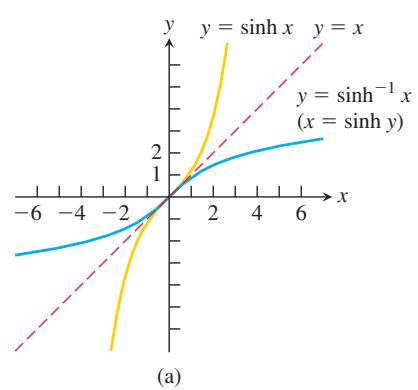
For every value of x in the interval $- \infty < 𝑥 < \infty$ , the value of $𝑦 = s i n h - 1 𝑥$ is the number whose hyperbolic sine is x. The graphs of $𝑦 = s i n h 𝑥$ and $𝑦 = s i n h - 1 𝑥$ are shown in Figure 7.8a. Other notations used for the inverse hyperbolic sine function include arcsinh x, arsinh x, and argsinh x.

The function $𝑦 = c o s h 𝑥$ is not one-to-one because its graph in Table 7.4 does not pass the horizontal line test. The restricted function $𝑦 = c o s h 𝑥, 𝑥 \geq 0$ , however, is one-to-one and therefore has an inverse, denoted by

𝑦 = c o s h - 1 𝑥 .

教材插图

(b)

教材插图

(c)

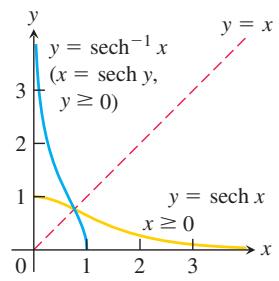
FIGURE 7.8 The graphs of the inverse hyperbolic sine, cosine, and secant of x. Notice the symmetries about the line y = x.

(c)

For every value of $𝑥 \geq 1$ , $𝑦 = c o s h - 1 𝑥$ is the number in the interval $0 \leq 𝑦 < \infty$ whose hyperbolic cosine is x. The graphs of $𝑦 = c o s h 𝑥, 𝑥 \geq 0$ , and $𝑦 = c o s h - 1 𝑥$ are shown in Figure 7.8b.

Like $𝑦 = c o s h 𝑥$ , the function $𝑦 = s e c h 𝑥 = 1 / c o s h 𝑥$ fails to be one-to-one, but its restriction to nonnegative values of x does have an inverse, denoted by

𝑦 = s e c h - 1 𝑥 .

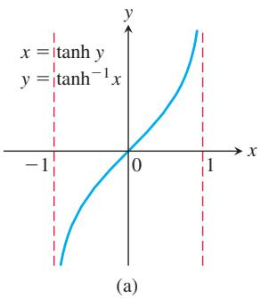
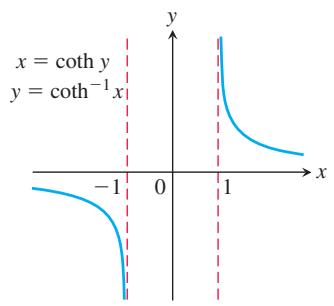
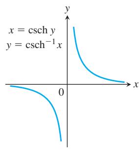
For every value of x in the interval $(0, 1]$ , $𝑦 = s e c h - 1 𝑥$ is the nonnegative number whose hyperbolic secant is x. The graphs of $𝑦 = s e c h 𝑥, 𝑥 \geq 0$ , and $𝑦 = s e c h - 1 𝑥$ are shown in Figure 7.8c.

The hyperbolic tangent, cotangent, and cosecant are one-to-one on their domains and therefore have inverses, denoted by

𝑦 = t a n h - 1 𝑥, 𝑦 = c o t h - 1 𝑥, 𝑦 = c s c h - 1 𝑥 .

These functions are graphed in Figure 7.9.

教材插图

(b)

FIGURE 7.9 The graphs of the inverse hyperbolic tangent, cotangent, and cosecant of x.

Useful Identities

TABLE 7.8 Identities for inverse hyperbolic functions

s e c h - 1 𝑥 = c o s h - 1 1 𝑥

c s c h - 1 𝑥 = s i n h - 1 1 𝑥

We can use the identities in Table 7.8 to express $s e c h - 1 𝑥$ , $c s c h - 1 𝑥$ , and $c o t h - 1 𝑥$ in terms of $c o s h - 1 𝑥$ , $s i n h - 1 𝑥$ , and $t a n h - 1 𝑥$ . These identities are direct consequences of the definitions. For example, if $0 < 𝑥 \leq 1$ , then

c o t h - 1 𝑥 = t a n h - 1 1 𝑥

s e c h (c o s h - 1 (1 𝑥)) = 1 c o s h (c o s h - 1 (1 𝑥)) = 1 (1 𝑥) = 𝑥 .

We also know that $s e c h (s e c h - 1 𝑥) = 𝑥$ , so because the hyperbolic secant is one-to-one on $(0, 1]$ , we have

c o s h - 1 (1 𝑥) = s e c h - 1 𝑥 .

Derivatives of Inverse Hyperbolic Functions

An important use of inverse hyperbolic functions lies in antiderivatives that reverse the derivative formulas in Table 7.9.

The restrictions $| 𝑥 | < 1$ and $| 𝑥 | > 1$ on the derivative formulas for $t a n h - 1 𝑥$ and $c o t h - 1 𝑥$ come from the natural restrictions on the values of these functions. (See Figure 7.9a and b.) The distinction between $| 𝑥 | < 1$ and $| 𝑥 | > 1$ becomes important when we convert the derivative formulas into integral formulas.

We illustrate how the derivatives of the inverse hyperbolic functions are found in Example 2, where we calculate $𝑑 (c o s h - 1 𝑥) / 𝑑 𝑥$ . The other derivatives are obtained by similar calculations.

TABLE 7.9 Derivatives of inverse hyperbolic functions

𝑑 (s i n h - 1 𝑥) 𝑑 𝑥 = 1 \sqrt 1 + 𝑥 2 𝑑 (c o s h - 1 𝑥) 𝑑 𝑥 = 1 \sqrt 𝑥 2 - 1, 𝑥 > 1 𝑑 (t a n h - 1 𝑥) 𝑑 𝑥 = 1 1 - 𝑥 2, | 𝑥 | < 1 𝑑 (c o t h - 1 𝑥) 𝑑 𝑥 = 1 1 - 𝑥 2, | 𝑥 | > 1 𝑑 (s e c h - 1 𝑥) 𝑑 𝑥 = - 1 𝑥 \sqrt 1 - 𝑥 2, 0 < 𝑥 < 1 𝑑 (c s c h - 1 𝑥) 𝑑 𝑥 = - 1 | 𝑥 | \sqrt 1 + 𝑥 2, 𝑥 \neq 0

EXAMPLE 2 Show that if $𝑥$ is greater than 1, then

𝑑 𝑑 𝑥 (c o s h - 1 𝑥) = 1 \sqrt 𝑥 2 - 1 .

Solution We find the derivative of $𝑦 = c o s h - 1 𝑥$ for x > 1 by applying Theorem 3 of Section 3.8 with $𝑓 (𝑥) = c o s h 𝑥$ and $𝑓 - 1 (𝑥) = c o s h - 1 𝑥$ . Theorem 3 can be applied because the derivative of $c o s h 𝑥$ is positive when x > 0.

(𝑓 - 1)' (𝑥) = 1 𝑓' (𝑓 - 1 (𝑥)) T h e o r e m 3, S e c t i o n 3.8 = 1 s i n h (c o s h - 1 𝑥) 𝑓' (𝑥) = s i n h 𝑥 = 1 \sqrt c o s h 2 (c o s h - 1 𝑥) - 1 c o s h 2 𝑥 - s i n h 2 𝑥 = 1, (𝑥 \geq 0), = 1 \sqrt 𝑥 2 - 1 s i n h 𝑥 = \sqrt c o s h 2 𝑥 - 1 c o s h (c o s h - 1 𝑥) = 𝑥

Kovalevsky, a Russian mathematician, primarily worked on the theory of partial differential equations, and a central result on the existence of solutions still bears her name. She published numerous papers on partial differential equations, eventually gaining recognition as the first woman to be elected a member of the Russian Imperial Academy of Sciences in 1889.

To know more, visit the companion Website.

With appropriate substitutions, the derivative formulas in Table 7.9 lead to the integration formulas in Table 7.10. Each of the formulas in Table 7.10 can be verified by differentiating the expression on the right-hand side.

EXAMPLE 3 Evaluate

\int 10 2 𝑑 𝑥 \sqrt 3 + 4 𝑥 2 .

TABLE 7.10 Integrals leading to inverse hyperbolic functions

\int 𝑑 𝑥 \sqrt 𝑎 2 + 𝑥 2 = s i n h - 1 (𝑥 𝑎) + 𝐶,

𝑎 > 0

$\int 𝑑 𝑥 \sqrt 𝑥 2 - 𝑎 2 = c o s h - 1 (𝑥 𝑎) + 𝐶,$

𝑥 > 𝑎 > 0

\int 𝑑 𝑥 𝑎 2 - 𝑥 2 = {1 𝑎 t a n h - 1 (𝑥 𝑎) + 𝐶, 1 𝑎 c o t h - 1 (𝑥 𝑎) + 𝐶,

𝑥 2 < 𝑎 2

𝑥 2 > 𝑎 2

\int 𝑑 𝑥 𝑥 \sqrt 𝑎 2 - 𝑥 2 = - 1 𝑎 s e c h - 1 (𝑥 𝑎) + 𝐶, 0 < 𝑥 < 𝑎

\int 𝑑 𝑥 𝑥 \sqrt 𝑎 2 + 𝑥 2 = - 1 𝑎 c s c h - 1 ∣ 𝑥 𝑎 ∣ + 𝐶, 𝑥 \neq 0 a n d 𝑎 > 0

Solution The indefinite integral is

\int 2 𝑑 𝑥 \sqrt 3 + 4 𝑥 2 = \int 𝑑 𝑢 \sqrt 3 + 𝑢 2 𝑢 = 2 𝑥, 𝑑 𝑢 = 2 𝑑 𝑥 = s i n h - 1 (𝑢 \sqrt 3) + 𝐶 F o r m u l a 1 f r o m T a b l e 7.10 w i t h 𝑎 2 = 3 = s i n h - 1 (2 𝑥 \sqrt 3) + 𝐶 .

Therefore,

\int 10 2 𝑑 𝑥 \sqrt 3 + 4 𝑥 2 = [s i n h - 1 (2 𝑥 \sqrt 3)] 10 = s i n h - 1 (2 \sqrt 3) - s i n h - 1 (0) = s i n h - 1 (2 \sqrt 3) - 0 \approx 0 . 9866 5 .

EXERCISES 7.3

Values and Identities

Each of Exercises 1–4 gives a value of $s i n h 𝑥$ or $c o s h 𝑥$ . Use the definitions and the identity $c o s h 2 𝑥 - s i n h 2 𝑥 = 1$ to find the values of the remaining five hyperbolic functions.

$s i n h 𝑥 = - 34$
$s i n h 𝑥 = 43$
$c o s h 𝑥 = 1715, 𝑥 > 0$
$c o s h 𝑥 = 135, 𝑥 > 0$

Rewrite the expressions in Exercises 5–10 in terms of exponentials and simplify the results as much as you can.

Then use them to show that

a. $s i n h 2 𝑥 = 2 s i n h 𝑥 c o s h 𝑥 .$

b. $c o s h 2 𝑥 = c o s h 2 𝑥 + s i n h 2 𝑥 .$

$2 c o s h (l n 𝑥)$
$c o s h 5 𝑥 + s i n h 5 𝑥$
$c o s h 3 𝑥 - s i n h 3 𝑥$

c o s h 2 𝑥 - s i n h 2 𝑥 = 1 .

$(s i n h 𝑥 + c o s h 𝑥) 4$
$l n (c o s h 𝑥 + s i n h 𝑥) + l n (c o s h 𝑥 - s i n h 𝑥)$
Prove the identities $s i n h (𝑥 + 𝑦) = s i n h 𝑥 c o s h 𝑦 + c o s h 𝑥 s i n h 𝑦,$ $c o s h (𝑥 + 𝑦) = c o s h 𝑥 c o s h 𝑦 + s i n h 𝑥 s i n h 𝑦 .$
Use the definitions of $c o s h 𝑥$ and $s i n h 𝑥$ to show that

Finding Derivatives

In Exercises 13–24, find the derivative of y with respect to the appropriate variable.

$𝑦 = 6 s i n h 𝑥 3$
$𝑦 = 12 s i n h (2 𝑥 + 1)$
$𝑦 = 2 \sqrt 𝑡$ $t a n h \sqrt 𝑡$
$𝑦 = 𝑡 2 t a n h 1 𝑡$
$𝑦 = l n (s i n h 𝑧)$
$𝑦 = l n (c o s h 𝑧)$
$𝑦 = (s e c h 𝜃) (1 - l n s e c h 𝜃)$
$𝑦 = (c s c h 𝜃) (1 - l n c s c h 𝜃)$
$𝑦 = l n c o s h 𝑣 - 12 t a n h 2 𝑣$
$𝑦 = l n s i n h 𝑣 - 12 c o t h 2 𝑣$
$𝑦 = (𝑥 2 + 1) s e c h (l n 𝑥)$

(Hint: Before differentiating, express in terms of exponentials and simplify.)

$𝑦 = (4 𝑥 2 - 1) c s c h (l n 2 𝑥)$

In Exercises 25–36, find the derivative of y with respect to the appropriate variable.

$𝑦 = s i n h - 1 \sqrt 𝑥$
$𝑦 = c o s h - 1 2 \sqrt 𝑥 + 1$
$𝑦 = (1 - 𝜃) t a n h - 1 𝜃$
$𝑦 = (𝜃 2 + 2 𝜃) t a n h - 1 (𝜃 + 1)$
$𝑦 = (1 - 𝑡) c o t h - 1 \sqrt 𝑡$
$𝑦 = (1 - 𝑡 2) c o t h - 1 𝑡$
$𝑦 = c o s - 1 𝑥 - 𝑥 s e c h - 1 𝑥$
$𝑦 = l n 𝑥 + \sqrt 1 - 𝑥 2$ $s e c h - 1 𝑥$
$𝑦 = c s c h - 1 (12) 𝜃$
$𝑦 = c s c h - 1 2 𝜃$
$𝑦 = s i n h - 1 (t a n 𝑥)$
$𝑦 = c o s h - 1 (s e c 𝑥), 0 < 𝑥 < 𝜋 / 2$

Integration Formulas

Verify the integration formulas in Exercises 37–40.

a. $\int s e c h 𝑥 𝑑 𝑥 = t a n - 1 (s i n h 𝑥) + 𝐶$

b. $\int s e c h 𝑥 𝑑 𝑥 = s i n - 1 (t a n h 𝑥) + 𝐶$

$\int 𝑥 s e c h - 1 𝑥 𝑑 𝑥 = 𝑥 2 2 s e c h - 1 𝑥 - 12 \sqrt 1 - 𝑥 2 + 𝐶$
$\int 𝑥 c o t h - 1 𝑥 𝑑 𝑥 = 𝑥 2 - 1 2 c o t h - 1 𝑥 + 𝑥 2 + 𝐶$
$\int t a n h - 1 𝑥 𝑑 𝑥 = 𝑥 t a n h - 1 𝑥 + 12 l n (1 - 𝑥 2) + 𝐶$

Evaluating Integrals

Evaluate the integrals in Exercises 41–60.

$\int s i n h 2 𝑥 𝑑 𝑥$
$\int s i n h 𝑥 5 𝑑 𝑥$
$\int 6 c o s h (𝑥 2 - l n 3) 𝑑 𝑥$
$\int 4 c o s h (3 𝑥 - l n 2) 𝑑 𝑥$
$\int t a n h 𝑥 7 𝑑 𝑥$
$\int c o t h 𝜃 \sqrt 3 𝑑 𝜃$
$\int s e c h 2 (𝑥 - 12) 𝑑 𝑥$
$\int c s c h 2 (5 - 𝑥) 𝑑 𝑥$
$\int s e c h \sqrt 𝑡 t a n h \sqrt 𝑡 𝑑 𝑡 \sqrt 𝑡$
$\int c s c h (l n 𝑡) c o t h (l n 𝑡) 𝑑 𝑡 𝑡$
$\int l n 4 l n 2 c o t h 𝑥 𝑑 𝑥$
$\int l n 2 0 t a n h 2 𝑥 𝑑 𝑥$
$\int - l n 2 - l n 4 2 𝑒 𝜃 c o s h 𝜃 𝑑 𝜃$
$\int l n 2 0 4 𝑒 - 𝜃 s i n h 𝜃 𝑑 𝜃$
$\int 𝜋 / 4 - 𝜋 / 4 c o s h (t a n 𝜃) s e c 2 𝜃 𝑑 𝜃$
$\int 𝜋 / 2 0 2 s i n h (s i n 𝜃) c o s 𝜃 𝑑 𝜃$
$\int 21 c o s h (l n 𝑡) 𝑡 𝑑 𝑡$
$\int 41 8 c o s h \sqrt 𝑥 \sqrt 𝑥 𝑑 𝑥$
$\int 0 - l n 2 c o s h 2 (𝑥 2) 𝑑 𝑥$
$\int l n 10 0 4 s i n h 2 (𝑥 2) 𝑑 𝑥$

Inverse Hyperbolic Functions and Integrals

Since the hyperbolic functions can be expressed in terms of exponential functions, it is possible to express the inverse hyperbolic functions in terms of logarithms, as shown in the following table.

$s i n h - 1 𝑥 = l n (𝑥 + \sqrt 𝑥 2 + 1)$

- \infty < 𝑥 < \infty

$c o s h - 1 𝑥 = l n (𝑥 + \sqrt 𝑥 2 - 1), 𝑥 \geq 1$

$t a n h - 1 𝑥 = 12 l n 1 + 𝑥 1 - 𝑥,$

$| 𝑥 | < 1$

$s e c h - 1 𝑥 = l n (1 + \sqrt 1 - 𝑥 2 𝑥),$

0 < 𝑥 \leq 1

c h - 1 𝑥 = l n (1 𝑥 + \sqrt 1 + 𝑥 2 | 𝑥 |),

$c o t h - 1 𝑥 = 12 l n 𝑥 + 1 𝑥 - 1,$

𝑥 \neq 0

$| 𝑥 | > 1$

Use these formulas to express the numbers in Exercises 61–66 in terms of natural logarithms.

$s i n h - 1 (- 5 / 12)$
$c o s h - 1 (5 / 3)$
$t a n h - 1 (- 1 / 2)$
$c o t h - 1 (5 / 4)$
$s e c h - 1 (3 / 5)$
$c s c h - 1 (- 1 / \sqrt 3)$

Evaluate the integrals in Exercises 67–74 in terms of a. inverse hyperbolic functions. b. natural logarithms.

$\int 2 \sqrt 3 0 𝑑 𝑥 \sqrt 4 + 𝑥 2$
$\int 1 / 3 0 6 𝑑 𝑥 \sqrt 1 + 9 𝑥 2$
$\int 2 5 / 4 𝑑 𝑥 1 - 𝑥 2$
$\int 1 / 2 0 𝑑 𝑥 1 - 𝑥 2$
$\int 3 / 13 1 / 5 𝑑 𝑥 𝑥 \sqrt 1 - 16 𝑥 2$
$\int 21 𝑑 𝑥 𝑥 \sqrt 4 + 𝑥 2$
$\int 𝜋 0 c o s 𝑥 𝑑 𝑥 \sqrt 1 + s i n 2 𝑥$
$\int 𝑒 1 𝑑 𝑥 𝑥 \sqrt 1 + (l n 𝑥) 2$

Applications and Examples

Show that if a function $𝑓$ is defined on an interval symmetric about the origin (so that $𝑓$ is defined at $- 𝑥$ whenever it is defined at $𝑥$ ), then

𝑓 (𝑥) = 𝑓 (𝑥) + 𝑓 (- 𝑥) 2 + 𝑓 (𝑥) - 𝑓 (- 𝑥) 2 .

Then show that $(𝑓 (𝑥) + 𝑓 (- 𝑥)) / 2$ is even and that $(𝑓 (𝑥) - 𝑓 (- 𝑥)) / 2$ is odd.

Derive the formula $s i n h - 1 𝑥 = l n (𝑥 + \sqrt 𝑥 2 + 1)$ for all real x. Explain in your derivation why the plus sign is used with the square root instead of the minus sign.
Skydiving If a body of mass $𝑚$ falling from rest under the action of gravity encounters an air resistance proportional to the square of the velocity, then the body’s velocity $𝑡$ s into the fall satisfies the differential equation

𝑚 𝑑 𝑣 𝑑 𝑡 = 𝑚 𝑔 - 𝑘 𝑣 2,

where $𝑘$ is a constant that depends on the body’s aerodynamic properties and the density of the air. (We assume that the fall is short enough so that the variation in the air’s density will not affect the outcome significantly.)

a. Show that

𝑣 = \sqrt 𝑚 𝑔 𝑘 t a n h (\sqrt 𝑔 𝑘 𝑚 𝑡)

satisfies the differential equation and the initial condition that v = 0 when t = 0.

b. Find the body’s limiting velocity, $l i m 𝑡 \to \infty 𝑣$

c. For a 75-kg skydiver (mg = 735 N), with time in seconds and distance in meters, a typical value for k is 0.235. What is the diver’s limiting velocity?

Accelerations whose magnitudes are proportional to displacement Suppose that the position of a body moving along a coordinate line at time t is

a. $𝑠 = 𝑎 c o s 𝑘 𝑡 + 𝑏 s i n 𝑘 𝑡$ . b. $𝑠 = 𝑎 c o s h 𝑘 𝑡 + 𝑏 s i n h 𝑘 𝑡$ .

Show in both cases that the acceleration $𝑑 2 𝑠 / 𝑑 𝑡 2$ is proportional to s but that in the first case it is directed toward the origin, whereas in the second case it is directed away from the origin.

Volume A region in the first quadrant is bounded above by the curve $𝑦 = c o s h 𝑥$ , below by the curve $𝑦 = s i n h 𝑥$ , and on the left and right by the y-axis and the line x = 2, respectively. Find the volume of the solid generated by revolving the region about the x-axis.
Volume The region enclosed by the curve y = sech x, the x-axis, and the lines $𝑥 = \pm l n \sqrt 3$ is revolved about the x-axis to generate a solid. Find the volume of the solid.
Arc length Find the length of the graph of $𝑦 = (1 / 2) c o s h 2 𝑥$ from x = 0 to $𝑥 = l n \sqrt 5$ .
Use the definitions of the hyperbolic functions to find each of the following limits.

a. $l i m 𝑥 \to \infty t a n h 𝑥$

b. $l i m 𝑥 \to - \infty t a n h 𝑥$

c. $l i m 𝑥 \to \infty s i n h 𝑥$

d. $l i m 𝑥 \to - \infty s i n h 𝑥$

e. $l i m 𝑥 \to \infty$ sech x

g. $l i m 𝑥 \to 0 + c o t h 𝑥$ f. $l i m 𝑥 \to \infty c o t h 𝑥$

i. $l i m 𝑥 \to - \infty$ csch x

h. $l i m 𝑥 \to 0 - c o t h 𝑥$

Hanging cables Imagine a cable, like a telephone line or TV cable, strung from one support to another and hanging freely. The cable’s weight per unit length is a constant $𝑤$ , and the horizontal tension at its lowest point is a vector of length $𝐻$ . If we choose a coordinate system for the plane of the cable in which the $𝑥$ -axis is horizontal, the force of gravity is straight down, the positive $𝑦$ -axis points straight up, and the lowest point of the cable lies at the point $𝑦 = 𝐻 / 𝑤$ on the $𝑦$ -axis (see accompanying figure), then it can be shown that the cable lies along the graph of the hyperbolic cosine

𝑦 = 𝐻 𝑤 c o s h 𝑤 𝐻 𝑥 .

教材插图

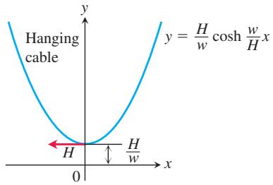
Such a curve is sometimes called a chain curve or a catenary, the latter deriving from the Latin catena, meaning “chain.”

a. Let $𝑃 (𝑥, 𝑦)$ denote an arbitrary point on the cable. The next accompanying figure displays the tension at $𝑃$ as a vector of length (magnitude) $𝑇$ , as well as the tension $𝐻$ at the lowest point $𝐴$ . Show that the cable’s slope at $𝑃$ is

t a n 𝜙 = 𝑑 𝑦 𝑑 𝑥 = s i n h 𝑤 𝐻 𝑥 .

教材插图

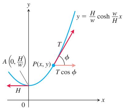
b. Using the result from part (a) and the fact that the horizontal tension at P must equal H (the cable is not moving), show that T = wy. Hence, the magnitude of the tension at $𝑃 (𝑥, 𝑦)$ is exactly equal to the weight of y units of cable.

(Continuation of Exercise 83.) The length of arc AP in the Exercise 83 figure is $𝑠 = (1 / 𝑎) s i n h 𝑎 𝑥$ , where a = w/H. Show that the coordinates of P may be expressed in terms of s as

𝑥 = 1 𝑎 s i n h - 1 𝑎 𝑠, 𝑦 = \sqrt 𝑠 2 + 1 𝑎 2 .

Area Show that the area of the region in the first quadrant enclosed by the curve $𝑦 = (1 / 𝑎) c o s h 𝑎 𝑥$ , the coordinate axes, and the line x = b is the same as the area of a rectangle of height 1/a and length s, where s is the length of the curve from x = 0 to x = b. Draw a figure illustrating this result.
The hyperbolic in hyperbolic functions Just as $𝑥 = c o s 𝑢$ and $𝑦 = s i n 𝑢$ are identified with points $(𝑥, 𝑦)$ on the unit circle, the functions $𝑥 = c o s h 𝑢$ and $𝑦 = s i n h 𝑢$ are identified with points $(𝑥, 𝑦)$ on the right-hand branch of the unit hyperbola, $𝑥 2 - 𝑦 2 = 1$ .

教材插图

2 𝑢 - s i n h 2 𝑢 = 1,

𝑥 2 - 𝑦 2 = 1

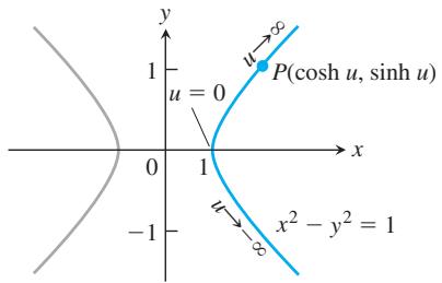
Another analogy between hyperbolic and circular functions is that the variable u in the coordinates $(c o s h 𝑢, s i n h 𝑢)$ for the points of the right-hand branch of the hyperbola $𝑥 2 - 𝑦 2 = 1$ is twice the area of the sector AOP pictured in the figure following part (c). To see why this is so, carry out the following steps.

a. Show that the area $𝐴 (𝑢)$ of sector AOP is

𝐴 (𝑢) = 12 c o s h 𝑢 s i n h 𝑢 - \int c o s h 𝑢 1 \sqrt 𝑥 2 - 1 𝑑 𝑥 .

b. Differentiate both sides of the equation in part (a) with respect to $𝑢$ to show that

𝐴' (𝑢) = 12 .

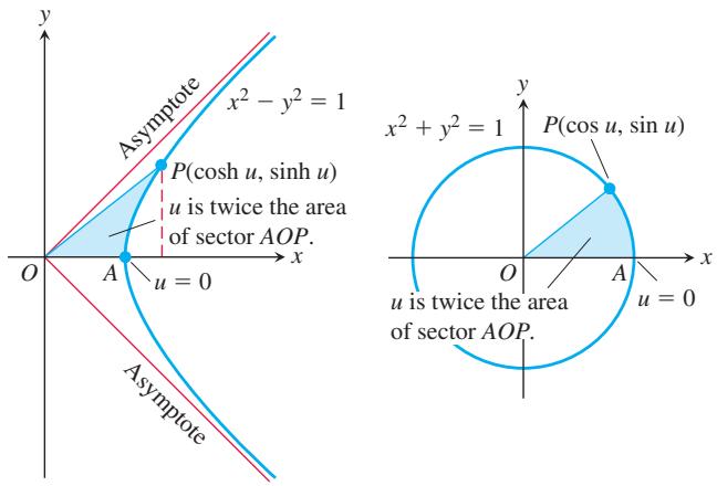
c. Solve this last equation for $𝐴 (𝑢)$ . What is the value of $𝐴 (0)$ ? What is the value of the constant of integration $𝐶$ in your solution? With $𝐶$ determined, what does your solution say about the relationship of $𝑢$ to $𝐴 (𝑢)$ ?

教材插图

One of the analogies between hyperbolic and circular functions is revealed by these two diagrams (Exercise 86).

7.4 Relative Rates of Growth

教材插图

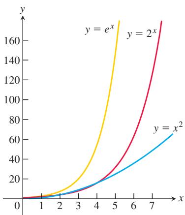
FIGURE 7.10 The graphs of $𝑒 𝑥, 2 𝑥$ , and $𝑥 2$ .

It is often important in mathematics, computer science, and engineering to compare the rates at which functions of x grow as x becomes large. Exponential functions are important in these comparisons because of their very fast growth, and logarithmic functions because of their very slow growth. In this section we introduce the little-oh and big-oh notation used to describe the results of these comparisons. We restrict our attention to functions whose values eventually become and remain positive as $𝑥 \to \infty$ .

Growth Rates of Functions

You may have noticed that exponential functions like $2 𝑥$ and $𝑒 𝑥$ seem to grow more rapidly as x gets large than do polynomials and rational functions. These exponentials certainly grow more rapidly than x itself, and you can see $2 𝑥$ outgrowing $𝑥 2$ as x increases in Figure 7.10. In fact, as $𝑥 \to \infty$ , the functions $2 𝑥$ and $𝑒 𝑥$ grow faster than any power of x, even $𝑥 1, 000, 000$ (Exercise 19). In contrast, logarithmic functions like $𝑦 = l o g 2 𝑥$ and $𝑦 = l n 𝑥$ grow more slowly as $𝑥 \to \infty$ than any positive power of x (Exercise 21).

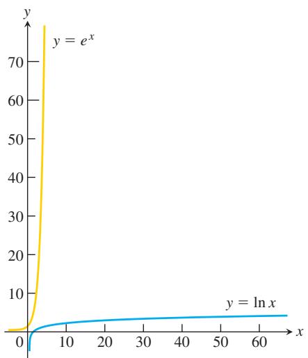
To get a feeling for how rapidly the values of $𝑦 = 𝑒 𝑥$ grow with increasing $𝑥$ , think of graphing the function on a large blackboard, with the axes scaled in centimeters. At $𝑥 = 1 c m$ , the graph is $𝑒 1 \approx 3 c m$ above the $𝑥$ -axis. At $𝑥 = 6 c m$ , the graph is $𝑒 6 \approx 403 c m \approx 4 m$ high (it is about to go through the ceiling if it hasn’t done so already). At $𝑥 = 10 c m$ , the graph is $𝑒 10 \approx 22, 026 c m \approx 220 m$ high, higher than most buildings. At $𝑥 = 24 c m$ , the graph is more than halfway to the moon, and at $𝑥 = 43 c m$ from the origin, the graph is high enough to reach past the sun’s closest stellar neighbor, the red dwarf star Proxima Centauri. By contrast, with axes scaled in centimeters, you have to go nearly 5 light-years out on the $𝑥$ -axis to find a point where the graph of $𝑦 = l n 𝑥$ is even $𝑦 = 43 c m$ high. See Figure 7.11.

教材插图

FIGURE 7.11 Scale drawings of the graphs of $𝑒 𝑥$ and $l n 𝑥$ .

These important comparisons of exponential, polynomial, and logarithmic functions can be made precise by defining what it means for a function $𝑓 (𝑥)$ to grow faster than another function $𝑔 (𝑥)$ as $𝑥 \to \infty$ .

DEFINITION Let $𝑓 (𝑥)$ and $𝑔 (𝑥)$ be positive for x sufficiently large.

1. $𝑓$ grows faster than $𝑔$ as $𝑥 \to \infty$ if
$l i m 𝑥 \to \infty 𝑓 (𝑥) 𝑔 (𝑥) = \infty$
or, equivalently, if
$l i m 𝑥 \to \infty 𝑔 (𝑥) 𝑓 (𝑥) = 0 .$
We also say that $𝑔$ grows slower than $𝑓$ as $𝑥 \to \infty$ .

$𝑓$ and $𝑔$ grow at the same rate as $𝑥 \to \infty$ if

$l i m 𝑥 \to \infty 𝑓 (𝑥) 𝑔 (𝑥) = 𝐿$
where $𝐿$ is finite and positive.

According to these definitions, $𝑦 = 2 𝑥$ does not grow faster than $𝑦 = 𝑥$ . The two functions grow at the same rate because

l i m 𝑥 \to \infty 2 𝑥 𝑥 = l i m 𝑥 \to \infty 2 = 2,

which is a finite, positive limit. The reason for this departure from more colloquial usage is that we want “f grows faster than g” to mean that for large x-values g is negligible when compared with f.

EXAMPLE 1 We compare the growth rates of several common functions.

(a) $𝑒 𝑥$ grows faster than $𝑥 2$ as $𝑥 \to \infty$ because

l i m 𝑥 \to \infty 𝑒 𝑥 𝑥 2 ⏟ \infty / \infty = l i m 𝑥 \to \infty 𝑒 𝑥 2 𝑥 ⏟ \infty / \infty = l i m 𝑥 \to \infty 𝑒 𝑥 2 = \infty . U s i n g l' H ô p i t a l' s R u l e t w i c e

(b) $3 𝑥$ grows faster than $2 𝑥$ as $𝑥 \to \infty$ because

l i m 𝑥 \to \infty 3 𝑥 2 𝑥 = l i m 𝑥 \to \infty (32) 𝑥 = \infty .

l i m 𝑥 \to \infty 𝑥 2 l n 𝑥 = l i m 𝑥 \to \infty 2 𝑥 1 / 𝑥 = l i m 𝑥 \to \infty 2 𝑥 2 = \infty . l' H ô p i t a l' s R u l e

(d) In x grows slower than $𝑥 1 / 𝑛$ as $𝑥 \to \infty$ for any positive integer n because

l i m 𝑥 \to \infty l n 𝑥 𝑥 1 / 𝑛 = l i m 𝑥 \to \infty 1 / 𝑥 (1 / 𝑛) 𝑥 (1 / 𝑛) - 1 l' H ô p i t a l' s R u l e = l i m 𝑥 \to \infty 𝑛 𝑥 1 / 𝑛 = 0 . n i s c o n s t a n t .

(e) As part (b) suggests, exponential functions with different bases never grow at the same rate as $𝑥 \to \infty$ . If a > b > 0, then $𝑎 𝑥$ grows faster than $𝑏 𝑥$ . Since $(𝑎 / 𝑏) > 1$ ,

l i m 𝑥 \to \infty 𝑎 𝑥 𝑏 𝑥 = l i m 𝑥 \to \infty (𝑎 𝑏) 𝑥 = \infty .

(f) In contrast to exponential functions, logarithmic functions with different bases $𝑎 > 1$ and $𝑏 > 1$ always grow at the same rate as $𝑥 \to \infty$ :

l i m 𝑥 \to \infty l o g 𝑎 𝑥 l o g 𝑏 𝑥 = l i m 𝑥 \to \infty l n 𝑥 / l n 𝑎 l n 𝑥 / l n 𝑏 = l n 𝑏 l n 𝑎 .

The limiting ratio is always finite and never zero.

If $𝑓$ grows at the same rate as $𝑔$ as $𝑥 \to \infty$ , and $𝑔$ grows at the same rate as $ℎ$ as $𝑥 \to \infty$ , then $𝑓$ grows at the same rate as $ℎ$ as $𝑥 \to \infty$ . The reason is that

l i m 𝑥 \to \infty 𝑓 𝑔 = 𝐿 1 a n d l i m 𝑥 \to \infty 𝑔 ℎ = 𝐿 2

together imply

l i m 𝑥 \to \infty 𝑓 ℎ = l i m 𝑥 \to \infty 𝑓 𝑔 \cdot 𝑔 ℎ = 𝐿 1 𝐿 2 .

If $𝐿 1$ and $𝐿 2$ are finite and nonzero, then so is $𝐿 1 𝐿 2$ .

EXAMPLE 2 Show that $\sqrt 𝑥 2 + 5$ and $(2 \sqrt 𝑥 - 1) 2$ grow at the same rate as $𝑥 \to \infty$ .

Solution We show that the functions grow at the same rate by showing that they both grow at the same rate as the function $𝑔 (𝑥) = 𝑥$ :

l i m 𝑥 \to \infty \sqrt 𝑥 2 + 5 𝑥 = l i m 𝑥 \to \infty \sqrt 1 + 5 𝑥 2 = 1,

l i m 𝑥 \to \infty (2 \sqrt 𝑥 - 1) 2 𝑥 = l i m 𝑥 \to \infty (2 \sqrt 𝑥 - 1 \sqrt 𝑥) 2 = l i m 𝑥 \to \infty (2 - 1 \sqrt 𝑥) 2 = 4 .

Order and Oh-Notation

The “little-oh” and “big-oh” notation was invented by number theorists over a hundred years ago and is now commonplace in mathematical analysis and computer science. According to this definition, saying $𝑓 = 𝑜 (𝑔)$ as $𝑥 \to \infty$ is another way to say that f grows slower than g as $𝑥 \to \infty$ .

DEFINITION A function $𝑓$ is of smaller order than $𝑔$ as $𝑥 \to \infty$ if $l i m 𝑥 \to \infty 𝑓 (𝑥) 𝑔 (𝑥) = 0$ . We indicate this by writing $𝑓 = 𝑜 (𝑔)$ (” $𝑓$ is little-oh of $𝑔$ ”).

EXAMPLE 3 Here we use little-oh notation.

(a) l n 𝑥 = 𝑜 (𝑥) a s 𝑥 \to \infty b e c a u s e l i m 𝑥 \to \infty l n 𝑥 𝑥 = 0

(b) 𝑥 2 = 𝑜 (𝑥 3 + 1) a s 𝑥 \to \infty b e c a u s e l i m 𝑥 \to \infty 𝑥 2 𝑥 3 + 1 = 0

DEFINITION Let $𝑓 (𝑥)$ and $𝑔 (𝑥)$ be positive for $𝑥$ sufficiently large. Then $𝑓$ is of at most the order of $𝑔$ as $𝑥 \to \infty$ if there is a positive integer $𝑀$ for which
$𝑓 (𝑥) 𝑔 (𝑥) \leq 𝑀,$

for $𝑥$ sufficiently large. We indicate this by writing $𝑓 = 𝑂 (𝑔)$ (” $𝑓$ is big-oh of $𝑔$ ”).

EXAMPLE 4 Here we use big-oh notation.

(a) 𝑥 + s i n 𝑥 = 𝑂 (𝑥) a s 𝑥 \to \infty b e c a u s e 𝑥 + s i n 𝑥 𝑥 \leq 2 f o r 𝑥 s u f f i c i e n t l y l a r g e .

(𝐛) 𝑒 𝑥 + 𝑥 2 = 𝑂 (𝑒 𝑥) a s 𝑥 \to \infty b e c a u s e 𝑒 𝑥 + 𝑥 2 𝑒 𝑥 \to 1 a s 𝑥 \to \infty .

(𝐜) 𝑥 = 𝑂 (𝑒 𝑥) a s 𝑥 \to \infty b e c a u s e 𝑥 𝑒 𝑥 \to 0 a s 𝑥 \to \infty .

If you look at the definitions again, you will see that $𝑓 = 𝑜 (𝑔)$ implies $𝑓 = 𝑂 (𝑔)$ for functions that are positive for all sufficiently large x. Also, if f and g grow at the same rate, then $𝑓 = 𝑂 (𝑔)$ and $𝑔 = 𝑂 (𝑓)$ (Exercise 11).

Sequential vs. Binary Search

Computer scientists often measure the efficiency of an algorithm by counting the number of steps a computer must take to execute the algorithm. There can be significant differences in how efficiently algorithms perform, even if they are designed to accomplish the same task. These differences are often described using big-oh notation. Here is an example.

One edition of Webster’s International Dictionary lists about 26,000 words that begin with the letter $𝑎$ . One way to look up a word, or to learn if it is not there, is to read through the list one word at a time until you either find the word or determine that it is not there. This method, called sequential search, makes no particular use of the words’ alphabetical arrangement in the list. You are sure to get an answer, but it might take 26,000 steps.

Another way to find the word or to learn it is not there is to go straight to the middle of the list (give or take a few words). If you do not find the word, then go to the middle of the half that contains it and forget about the half that does not. (You know which half contains it because you know the list is ordered alphabetically.) This method, called a binary search, eliminates roughly 13,000 words in a single step. If you do not find the word on the second try, then jump to the middle of the half that contains it. Continue this way until you have either found the word or divided the list in half so many times there are no words left. How many times do you have to divide the list to find the word or learn that it is not there? At most 15, because

(26, 000 / 215) < 1 .

That certainly beats a possible 26,000 steps.

For a list of length n, a sequential search algorithm takes on the order of n steps to find a word or determine that it is not in the list. A binary search, as the second algorithm is called, takes on the order of $l o g 2 𝑛$ steps. The reason is that if $2 𝑚 - 1 < 𝑛 \leq 2 𝑚$ , then $𝑚 - 1 < l o g 2 𝑛 \leq 𝑚$ , and the number of bisections required to narrow the list to one word will be at most $𝑚 = ⌈ l o g 2 𝑛 ⌉$ , the integer ceiling of the number $l o g 2 𝑛$ .

Big-oh notation provides a compact way to say all this. The number of steps in a sequential search of an ordered list is $𝑂 (𝑛)$ ; the number of steps in a binary search is $𝑂 (l o g 2 𝑛)$ . In our example, there is a big difference between the two (26,000 versus 15), and the difference can only increase with n because n grows faster than $l o g 2 𝑛$ as $𝑛 \to \infty$ .

EXERCISES 7.4

Comparisons with the Exponential $𝑒 𝑥$

Which of the following functions grow faster than $𝑒 𝑥$ as $𝑥 \to \infty$ ? Which grow at the same rate as $𝑒 𝑥$ ? Which grow slower? a. $𝑥 - 3$ b. $𝑥 3 + s i n 2 𝑥$ c. $\sqrt 𝑥$ d. $4 𝑥$ e. $(3 / 2) 𝑥$ f. $𝑒 𝑥 / 2$ g. $𝑒 𝑥 / 2$ h. $l o g 10 𝑥$
Which of the following functions grow faster than $𝑒 𝑥$ as $𝑥 \to \infty$ ? Which grow at the same rate as $𝑒 𝑥$ ? Which grow slower? a. $10 𝑥 4 + 30 𝑥 + 1$ b. $𝑥 l n 𝑥 - 𝑥$ c. $\sqrt 1 + 𝑥 4$ d. $(5 / 2) 𝑥$ e. $𝑒 - 𝑥$ f. $𝑥 𝑒 𝑥$ g. $𝑒 c o s 𝑥$ h. $𝑒 𝑥 - 1$

Comparisons with the Power $𝑥 2$

Which of the following functions grow faster than $𝑥 2$ as $𝑥 \to \infty$ ? Which grow at the same rate as $𝑥 2$ ? Which grow slower? a. $𝑥 2 + 4 𝑥$ b. $𝑥 5 - 𝑥 2$ c. $\sqrt 𝑥 4 + 𝑥 3$ d. $(𝑥 + 3) 2$ e. $𝑥 l n 𝑥$ f. $2 𝑥$ g. $𝑥 3 𝑒 - 𝑥$ h. $8 𝑥 2$
Which of the following functions grow faster than $𝑥 2$ as $𝑥 \to \infty$ ? Which grow at the same rate as $𝑥 2$ ? Which grow slower? a. $𝑥 2 + \sqrt 𝑥$ b. $10 𝑥 2$ c. $𝑥 2 𝑒 - 𝑥$ d. $l o g 10 (𝑥 2)$ e. $𝑥 3 - 𝑥 2$ f. $(1 / 10) 𝑥$ g. $(1.1) 𝑥$ h. $𝑥 2 + 100 𝑥$

Comparisons with the Logarithm In x

Which of the following functions grow faster than $l n 𝑥$ as $𝑥 \to \infty$ ? Which grow at the same rate as $l n 𝑥$ ? Which grow slower? a. $l o g 3 𝑥$ b. $l n 2 𝑥$ c. $l n \sqrt 𝑥$ d. $\sqrt 𝑥$ e. $𝑥$ f. $5 l n 𝑥$ g. $1 / 𝑥$ h. $𝑒 𝑥$
Which of the following functions grow faster than $l n 𝑥$ as $𝑥 \to \infty$ ? Which grow at the same rate as $l n 𝑥$ ? Which grow slower? a. $l o g 2 (𝑥 2)$ b. $l o g 10 10 𝑥$ c. $1 / \sqrt 𝑥$ d. $1 / 𝑥 2$ e. $𝑥 - 2 l n 𝑥$ f. $𝑒 - 𝑥$ g. $l n (l n 𝑥)$ h. $l n (2 𝑥 + 5)$

Ordering Functions by Growth Rates

Order the following functions from slowest growing to fastest growing as $𝑥 \to \infty$ . a. $𝑒 𝑥$ b. $𝑥 𝑥$ c. $(l n 𝑥) 𝑥$ d. $𝑒 𝑥 / 2$
Order the following functions from slowest growing to fastest growing as $𝑥 \to \infty$ . a. $2 𝑥$ b. $𝑥 2$ c. $(l n 2) 𝑥$ d. $𝑒 𝑥$

Big-oh and Little-oh; Order

True, or false? As $𝑥 \to \infty$ ,
a. $𝑥 = 𝑜 (𝑥)$ b. $𝑥 = 𝑜 (𝑥 + 5)$ c. $𝑥 = 𝑂 (𝑥 + 5)$ d. $𝑥 = 𝑂 (2 𝑥)$ e. $𝑒 𝑥 = 𝑜 (𝑒 2 𝑥)$ f. $𝑥 + l n 𝑥 = 𝑂 (𝑥)$ g. $l n 𝑥 = 𝑜 (l n 2 𝑥)$ h. $\sqrt 𝑥 2 + 5 = 𝑂 (𝑥)$
True, or false? As $𝑥 \to \infty$ ,
a. $1 𝑥 + 3 = 𝑂 (1 𝑥)$ b. $1 𝑥 + 1 𝑥 2 = 𝑂 (1 𝑥)$ c. $1 𝑥 - 1 𝑥 2 = 𝑜 (1 𝑥)$ d. $2 + c o s 𝑥 = 𝑂 (2)$ e. $𝑒 𝑥 + 𝑥 = 𝑂 (𝑒 𝑥)$ f. $𝑥 l n 𝑥 = 𝑜 (𝑥 2)$ g. $l n (l n 𝑥) = 𝑂 (l n 𝑥)$ h. $l n (𝑥) = 𝑜 (l n (𝑥 2 + 1))$
Show that if positive functions $𝑓 (𝑥)$ and $𝑔 (𝑥)$ grow at the same rate as $𝑥 \to \infty$ , then $𝑓 = 𝑂 (𝑔)$ and $𝑔 = 𝑂 (𝑓)$ .
When is a polynomial $𝑓 (𝑥)$ of smaller order than a polynomial $𝑔 (𝑥)$ as $𝑥 \to \infty$ ? Give reasons for your answer.
When is a polynomial $𝑓 (𝑥)$ of at most the order of a polynomial $𝑔 (𝑥)$ as $𝑥 \to \infty$ ? Give reasons for your answer.
What do the conclusions we drew in Section 2.8 about the limits of rational functions tell us about the relative growth of polynomials as $𝑥 \to \infty$ ?

Other Comparisons

T 15. Investigate

l i m 𝑥 \to \infty l n (𝑥 + 1) l n 𝑥

l i m 𝑥 \to \infty l n (𝑥 + 999) l n 𝑥 .

Then use l’Hôpital’s Rule to explain what you find.

(Continuation of Exercise 15.) Show that the value of

l i m 𝑥 \to \infty l n (𝑥 + 𝑎) l n 𝑥

is the same no matter what value you assign to the constant a. What does this say about the relative rates at which the functions $𝑓 (𝑥) = l n (𝑥 + 𝑎)$ and $𝑔 (𝑥) = l n 𝑥$ grow?

Show that $\sqrt 10 𝑥 + 1$ and $\sqrt 𝑥 + 1$ grow at the same rate as $𝑥 \to \infty$ by showing that they both grow at the same rate as $\sqrt 𝑥$ as $𝑥 \to \infty$ .
Show that $\sqrt 𝑥 4 + 𝑥$ and $\sqrt 𝑥 4 - 𝑥 3$ grow at the same rate as $𝑥 \to \infty$ by showing that they both grow at the same rate as $𝑥 2$ as $𝑥 \to \infty$ .
Show that $𝑒 𝑥$ grows faster as $𝑥 \to \infty$ than $𝑥 𝑛$ for any positive integer $𝑛$ , even $𝑥 1, 000, 000$ . (Hint: What is the $𝑛$ th derivative of $𝑥 𝑛$ ?)
The function $𝑒 𝑥$ outgrows any polynomial Show that $𝑒 𝑥$ grows faster as $𝑥 \to \infty$ than any polynomial

𝑎 𝑛 𝑥 𝑛 + 𝑎 𝑛 - 1 𝑥 𝑛 - 1 + \dots + 𝑎 1 𝑥 + 𝑎 0 .

a. Show that $l n 𝑥$ grows slower as $𝑥 \to \infty$ than $𝑥 1 / 𝑛$ for any positive integer $𝑛$ , even $𝑥 1 / 1, 000, 000$ .

T b. Although the values of $𝑥 1 / 1, 000, 000$ eventually overtake the values of $l n 𝑥$ , you have to go way out on the x-axis before this happens. Find a value of x greater than 1 for which $𝑥 1 / 1, 000, 000 > l n 𝑥$ . You might start by observing that when x > 1 the equation $l n 𝑥 = 𝑥 1 / 1, 000, 000$ is equivalent to the equation $l n (l n 𝑥) = (l n 𝑥) / 1, 000, 000$ .

T c. Even $𝑥 1 / 10$ takes a long time to overtake $l n 𝑥$ . Experiment with a calculator to find the value of x > 10 at which the graphs of $𝑥 1 / 10$ and $l n 𝑥$ cross, or, equivalently, at which $l n 𝑥 = 10 l n (l n 𝑥)$ . Bracket the crossing point between powers of 10 and then close in by successive halving.

CHAPTER 7 Questions to Guide Your Review

How is the natural logarithm function defined as an integral? What are its domain, range, and derivative? What arithmetic properties does it have? Comment on its graph.
What integrals lead to logarithms? Give examples.
What are the integrals of $t a n 𝑥$ and $c o t 𝑥$ ? Of $s e c 𝑥$ and $c s c 𝑥$ ?
How is the exponential function $𝑒 𝑥$ defined? What are its domain, range, and derivative? What laws of exponents does it obey? Comment on its graph.
How are the functions $𝑎 𝑥$ and $l o g 𝑎 𝑥$ defined? Are there any restrictions on $𝑎$ ? How is the graph of $l o g 𝑎 𝑥$ related to the graph of $l n 𝑥$ ? What truth is there in the statement that there are really only one exponential function and one logarithmic function?
How do you solve separable first-order differential equations?
What is the law of exponential change? How can it be derived from an initial value problem? What are some of the applications of the law?
What are the six basic hyperbolic functions? Comment on their domains, ranges, and graphs. What are some of the identities relating them?

T d. (Continuation of part (c).) The value of x at which $l n 𝑥 = 10 l n (l n 𝑥)$ is too far out for some graphers and root finders to identify. Try it on the equipment available to you and see what happens.

The function $l n 𝑥$ grows slower than any polynomial. Show that $l n 𝑥$ grows slower as $𝑥 \to \infty$ than any nonconstant polynomial.

Algorithms and Searches

a. Suppose you have three different algorithms for solving the same problem and each algorithm takes a number of steps that is of the order of one of the functions listed here:

𝑛 l o g 2 𝑛, 𝑛 3 / 2, 𝑛 (l o g 2 𝑛) 2 .

Which of the algorithms is the most efficient in the long run? Give reasons for your answer.

T b. Graph the functions in part (a) together to get a sense of how rapidly each one grows.

Repeat Exercise 23 for the functions

𝑛, \sqrt 𝑛 l o g 2 𝑛, (l o g 2 𝑛) 2 .

Suppose you are looking for an item in an ordered list one million items long. How many steps might it take to find that item with a sequential search? A binary search?
You are looking for an item in an ordered list 450,000 items long (the length of Webster’s Third New International Dictionary). How many steps might it take to find the item with a sequential search? A binary search?
What are the derivatives of the six basic hyperbolic functions? What are the corresponding integral formulas? What similarities do you see here to the six basic trigonometric functions?
How are the inverse hyperbolic functions defined? Comment on their domains, ranges, and graphs. How can you find values of $s e c h - 1 𝑥$ , $c s c h - 1 𝑥$ , and $c o t h - 1 𝑥$ using a calculator’s keys for $c o s h - 1 𝑥$ , $s i n h - 1 𝑥$ , and $t a n h - 1 𝑥$ ?
What integrals lead naturally to inverse hyperbolic functions?
How do you compare the growth rates of positive functions as $𝑥 \to \infty$ ?
What roles do the functions $𝑒 𝑥$ and $l n 𝑥$ play in growth comparisons?
Describe big-oh and little-oh notation. Give examples.
Which is more efficient—a sequential search or a binary search? Explain.

CHAPTER 7 Practice Exercises

Integration

Evaluate the integrals in Exercises 1–12.

$\int 𝑒 𝑥 s i n (𝑒 𝑥) 𝑑 𝑥$
$\int 𝑒 𝑡 c o s (3 𝑒 𝑡 - 2) 𝑑 𝑡$
$\int 𝜋 0 t a n 𝑥 3 𝑑 𝑥$
$\int 1 / 4 1 / 6 2 c o t 𝜋 𝑥 𝑑 𝑥$
$\int 𝜋 / 6 - 𝜋 / 2 c o s 𝑡 1 - s i n 𝑡 𝑑 𝑡$
$\int 𝑒 𝑥 s e c 𝑒 𝑥 𝑑 𝑥$
$\int l n (𝑥 - 5) 𝑥 - 5 𝑑 𝑥$
$\int c o s (1 - l n 𝑣) 𝑣 𝑑 𝑣$
$\int 71 3 𝑥 𝑑 𝑥$
$\int 321 1 5 𝑥 𝑑 𝑥$
$\int 𝑒 2 𝑒 1 𝑥 \sqrt l n 𝑥 𝑑 𝑥$
$\int 42 (1 + l n 𝑡) 𝑡 l n 𝑡 𝑑 𝑡$

Solving Equations with Logarithmic or Exponential Terms In Exercises 13–18, solve for y.

$3 𝑦 = 2 𝑦 + 1$
$4 - 𝑦 = 3 𝑦 + 2$

9 𝑒 2 𝑦 = 𝑥 2, 𝑥 > 0

$3 𝑦 = 3 l n 𝑥$
$l n (𝑦 - 1) = 𝑥 + l n 𝑦$
$l n (10 l n 𝑦) = l n 5 𝑥$

Comparing Growth Rates of Functions

Does $𝑓$ grow faster, slower, or at the same rate as $𝑔$ as $𝑥 \to \infty$ ? Give reasons for your answers. a. $𝑓 (𝑥) = l o g 2 𝑥$ , $𝑔 (𝑥) = l o g 3 𝑥$ b. $𝑓 (𝑥) = 𝑥$ , $𝑔 (𝑥) = 𝑥 + 1 𝑥$ c. $𝑓 (𝑥) = 𝑥 / 100$ , $𝑔 (𝑥) = 𝑥 𝑒 - 𝑥$ d. $𝑓 (𝑥) = 𝑥$ , $𝑔 (𝑥) = a r c t a n 𝑥$ e. $𝑓 (𝑥) = a r c c s c 𝑥$ , $𝑔 (𝑥) = 1 / 𝑥$ f. $𝑓 (𝑥) = s i n h 𝑥$ , $𝑔 (𝑥) = 𝑒 𝑥$
Does $𝑓$ grow faster, slower, or at the same rate as $𝑔$ as $𝑥 \to \infty$ ? Give reasons for your answers.

a. $𝑓 (𝑥) = 3 - 𝑥$ ,

𝑔 (𝑥) = 2 - 𝑥

𝑓 (𝑥) = l n 2 𝑥,

𝑔 (𝑥) = l n 𝑥 2

c. $𝑓 (𝑥) = 10 𝑥 3 + 2 𝑥 2,$

𝑔 (𝑥) = 𝑒 𝑥

d. $𝑓 (𝑥) = a r c t a n (1 / 𝑥)$ ,

𝑔 (𝑥) = 1 / 𝑥

e. $𝑓 (𝑥) = a r c s i n (1 / 𝑥)$ ,

𝑔 (𝑥) = 1 / 𝑥 2

f. $𝑓 (𝑥) = s e c h 𝑥,$

𝑔 (𝑥) = 𝑒 - 𝑥

True, or false? Give reasons for your answers.

a. $1 𝑥 2 + 1 𝑥 4 = 𝑂 (1 𝑥 2)$

1 𝑥 2 + 1 𝑥 4 = 𝑂 (1 𝑥 4)

c. $𝑥 = 𝑜 (𝑥 + l n 𝑥)$

d. $l n (l n 𝑥) = 𝑜 (l n 𝑥)$

e. $a r c t a n 𝑥 = 𝑂 (1)$

f. $c o s h 𝑥 = 𝑂 (𝑒 𝑥)$

True, or false? Give reasons for your answers. a. $1 𝑥 4 = 𝑂 (1 𝑥 2 + 1 𝑥 4)$ b. $1 𝑥 4 = 𝑜 (1 𝑥 2 + 1 𝑥 4)$ c. $l n 𝑥 = 𝑜 (𝑥 + 1)$ d. $l n 2 𝑥 = 𝑂 (l n 𝑥)$ e. $s e c - 1 𝑥 = 𝑂 (1)$ f. $s i n h 𝑥 = 𝑂 (𝑒 𝑥)$

Theory and Applications

The function $𝑓 (𝑥) = 𝑒 𝑥 + 𝑥$ , being differentiable and one-to-one, has a differentiable inverse $𝑓 - 1 (𝑥)$ . Find the value of $𝑑 𝑓 - 1 / 𝑑 𝑥$ at the point $𝑓 (l n 2)$ .
Find the inverse of the function $𝑓 (𝑥) = 1 + (1 / 𝑥), 𝑥 \neq 0$ . Then show that $𝑓 - 1 (𝑓 (𝑥)) = 𝑓 (𝑓 - 1 (𝑥)) = 𝑥$ and that

𝑑 𝑓 - 1 𝑑 𝑥 ∣ 𝑓 (𝑥) = 1 𝑓' (𝑥) .

A particle is traveling upward and to the right along the curve $𝑦 = l n 𝑥$ . Its x-coordinate is increasing at the rate $(𝑑 𝑥 / 𝑑 𝑡) = \sqrt 𝑥 m / s$ . At what rate is the y-coordinate changing at the point $(𝑒 2, 2)$ ?
A girl is sliding down a slide shaped like the curve $𝑦 = 3 𝑒 - 𝑥 / 3$ . Her $𝑦$ -coordinate is changing at the rate

𝑑 𝑦 / 𝑑 𝑡 = (- 1 / 4) \sqrt 3 - 𝑦 m / s .

At approximately what rate is her x-coordinate changing when she reaches the bottom of the slide at $𝑥 = 3 𝑚$ ?

The functions $𝑓 (𝑥) = l n 5 𝑥$ and $𝑔 (𝑥) = l n 3 𝑥$ differ by a constant. What constant? Give reasons for your answer.
a. If $(l n 𝑥) / 𝑥 = (l n 2) / 2$ , must $𝑥 = 2$ ? b. If $(l n 𝑥) / 𝑥 = - 2 l n 2$ , must $𝑥 = 1 / 2$ ? Give reasons for your answers.
The quotient $(l o g 4 𝑥) / (l o g 2 𝑥)$ has a constant value. What value? Give reasons for your answer.
$l o g 𝑥 (2)$ vs. $l o g 2 (𝑥)$ . How does $𝑓 (𝑥) = l o g 𝑥 (2)$ compare with $𝑔 (𝑥) = l o g 2 (𝑥)$ ? Here is one way to find out.

a. Use the equation $l o g 𝑎 𝑏 = (l n 𝑏) / (l n 𝑎)$ to express $𝑓 (𝑥)$ and $𝑔 (𝑥)$ in terms of natural logarithms.

b. Graph $𝑓$ and $𝑔$ together. Comment on the behavior of $𝑓$ in relation to the signs and values of $𝑔$ .

In Exercises 31–34, solve the differential equation.

$𝑑 𝑦 𝑑 𝑥 = \sqrt 𝑦 c o s 2 \sqrt 𝑦$
$𝑦' = 3 𝑦 (𝑥 + 1) 2 𝑦 - 1$
$𝑦 𝑦' = s e c 𝑦 2 s e c 2 𝑥$
$𝑦 c o s 2 𝑥 𝑑 𝑦 + s i n 𝑥 𝑑 𝑥 = 0$

In Exercises 35–38, solve the initial value problem.

$𝑑 𝑦 𝑑 𝑥 = 𝑒 - 𝑥 - 𝑦 - 2, 𝑦 (0) = - 2$
$𝑑 𝑦 𝑑 𝑥 = 𝑦 l n 𝑦 1 + 𝑥 2, 𝑦 (0) = 𝑒 2$
$𝑥 𝑑 𝑦 - (𝑦 + \sqrt 𝑦) 𝑑 𝑥 = 0, 𝑦 (1) = 1$
$𝑦 - 2 𝑑 𝑥 𝑑 𝑦 = 𝑒 𝑥 𝑒 2 𝑥 + 1, 𝑦 (0) = 1$
What is the age of a sample of charcoal in which 90% of the carbon-14 originally present has decayed?
Cooling a pie A deep-dish apple pie, whose internal temperature was $104 ° 𝐶$ when removed from the oven, was set out on a breezy $5 ° 𝐶$ porch to cool. Fifteen minutes later, the pie’s internal temperature was $82 ° 𝐶$ . How long did it take the pie to cool from there to $21 ° 𝐶$ ?
Find the length of the curve $𝑦 = l n (𝑒 𝑥 - 1) - l n (𝑒 𝑥 + 1)$ , $l n 2 \leq 𝑥 \leq l n 3$ .
In 1934, the Austrian biologist Ludwig von Bertalanffy derived and published the von Bertalanffy growth equation, which continues to be widely used and is especially important in fisheries studies. Let $𝐿 (𝑡)$ denote the length of a fish at time $𝑡$ and assume $𝐿 (0) = 𝐿 0$ . The von Bertalanffy equation is

𝑑 𝐿 𝑑 𝑡 = 𝑘 (𝐴 - 𝐿),

where $𝐴 = l i m 𝑡 \to \infty 𝐿 (𝑡)$ is the asymptotic length of the fish and k is a proportionality constant.

Assume that $𝐿 (𝑡)$ is the length in meters of a shark of age t years. In addition, assume A = 3, $𝐿 (0) = 0.5 m$ , and $𝐿 (5) = 1.75 m$ .

a. Solve the von Bertalanffy differential equation.

b. What is $𝐿 (10)$ ?

c. When does $𝐿 = 2.5 m$ ?

CHAPTER 7

Additional and Advanced Exercises

Let $𝐴 (𝑡)$ be the area of the region in the first quadrant enclosed by the coordinate axes, the curve $𝑦 = 𝑒 - 𝑥$ , and the vertical line $𝑥 = 𝑡, 𝑡 > 0$ . Let $𝑉 (𝑡)$ be the volume of the solid generated by revolving the region about the $𝑥$ -axis. Find the following limits. a. $l i m 𝑡 \to \infty 𝐴 (𝑡) 𝐛 . l i m 𝑡 \to \infty 𝑉 (𝑡) / 𝐴 (𝑡) 𝐜 . l i m 𝑡 \to 0 + 𝑉 (𝑡) / 𝐴 (𝑡)$
Varying a logarithm’s base

a. Find $l i m l o g 𝑎 2$ as $𝑎 \to 0 +, 1 -, 1 +$ , and $\infty$ .

T b. Graph $𝑦 = l o g 𝑎 2$ as a function of a over the interval $0 < 𝑎 \leq 4$ .

Graph $𝑓 (𝑥) = t a n - 1 𝑥 + t a n - 1 (1 / 𝑥)$ for $- 5 \leq 𝑥 \leq 5$ . Then use calculus to explain what you see. How would you expect $𝑓$ to behave beyond the interval $[- 5, 5]$ ? Give reasons for your answer.

T 4. Graph $𝑓 (𝑥) = (s i n 𝑥) s i n 𝑥$ over $[0, 3 𝜋]$ . Explain what you see.

Even-odd decompositions

a. Suppose that $𝑔$ is an even function of $𝑥$ and $ℎ$ is an odd function of $𝑥$ . Show that if $𝑔 (𝑥) + ℎ (𝑥) = 0$ for all $𝑥$ , then $𝑔 (𝑥) = 0$ for all $𝑥$ and $ℎ (𝑥) = 0$ for all $𝑥$ .

b. Use the result in part (a) to show that if $𝑓 (𝑥) = 𝑓 𝐸 (𝑥) + 𝑓 𝑂 (𝑥)$ is the sum of an even function $𝑓 𝐸 (𝑥)$ and an odd function $𝑓 𝑂 (𝑥)$ , then

𝑓 𝐸 (𝑥) = (𝑓 (𝑥) + 𝑓 (- 𝑥)) / 2

𝑓 𝑂 (𝑥) = (𝑓 (𝑥) - 𝑓 (- 𝑥)) / 2

c. What is the significance of the result in part (b)?

Let $𝑔$ be a function that is differentiable throughout an open interval containing the origin. Suppose $𝑔$ has the following properties. i. $𝑔 (𝑥 + 𝑦) = 𝑔 (𝑥) + 𝑔 (𝑦) 1 - 𝑔 (𝑥) 𝑔 (𝑦)$ for all real numbers $𝑥, 𝑦$ , and $𝑥 + 𝑦$ in the domain of $𝑔$ . ii. $l i m ℎ \to 0 𝑔 (ℎ) = 0$ iii. $l i m ℎ \to 0 𝑔 (ℎ) ℎ = 1$ a. Show that $𝑔 (0) = 0$ . b. Show that $𝑔' (𝑥) = 1 + [𝑔 (𝑥)] 2$ .

c. Find $𝑔 (𝑥)$ by solving the differential equation in part (b).

Center of mass Find the center of mass of a thin plate of constant density covering the region in the first and fourth quadrants enclosed by the curves $𝑦 = 1 / (1 + 𝑥 2)$ and $𝑦 = - 1 / (1 + 𝑥 2)$ and by the lines x = 0 and x = 1.
Solid of revolution The region between the curve $𝑦 = 1 / (2 \sqrt 𝑥)$ and the $𝑥$ -axis from $𝑥 = 1 / 4$ to $𝑥 = 4$ is revolved about the $𝑥$ -axis to generate a solid.

a. Find the volume of the solid.

b. Find the centroid of the region.

The Rule of 70 If you use the approximation $l n 2 \approx 0.70$ (in place of 0.69314 …), you can derive a rule of thumb that says, “To estimate how many years it will take an amount of money to double when invested at r percent compounded continuously, divide r into 70.” For instance, an amount of money invested at 5% will double in about 70/5 = 14 years. If you want it to double in 10 years instead, you have to invest it at 70/10 = 7%. Show how the Rule of 70 is derived. (A similar “Rule of 72” uses 72 instead of 70, because 72 has more integer factors.)
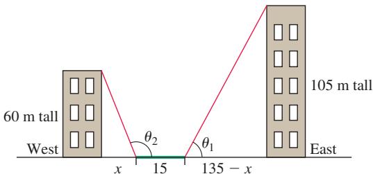
Urban gardening A vegetable garden 15 m wide is to be grown between two buildings, which are 150 m apart along an east-west line. If the buildings are 60 m and 105 m tall, where should the garden be placed in order to receive the maximum number of hours of sunlight exposure? (Hint: Determine the value of x in the accompanying figure that maximizes sunlight exposure for the garden.)

教材插图

Chapter 7: Integrals and Transcendental Functions

7.1 The Logarithm Defined as an Integral

Definition of the Natural Logarithm Function

The Graph and Range of ln⁡𝑥

The Integral ∫1/𝑥𝑑𝑥

The Inverse of ln⁡𝑥 and the Number 𝑒

The Derivative and Integral of 𝑒𝑥

Logarithms and Laws of Exponents

The General Exponential Function 𝑎𝑥

The General Power Function

Logarithms with Base 𝑎

Derivatives and Integrals Involving log𝑎⁡𝑥

Transcendental Numbers and Transcendental Functions

Summary

EXERCISES 7.1

Integration

Theory and Applications

Grapher Explorations

Calculations with Other Bases

7.2 Exponential Change and Separable Differential Equations

Exponential Change

Separable Differential Equations

Unlimited Population Growth

Radioactivity

Heat Transfer: Newton’s Law of Cooling

EXERCISES

Verifying Solutions

Initial Value Problems

Applications and Examples

7.3 Hyperbolic Functions

Definitions and Identities

Derivatives and Integrals of Hyperbolic Functions

Inverse Hyperbolic Functions

Useful Identities

Derivatives of Inverse Hyperbolic Functions

EXERCISES 7.3

Values and Identities

Finding Derivatives

Inverse Hyperbolic Functions and Integrals

Applications and Examples

7.4 Relative Rates of Growth

Growth Rates of Functions

DEFINITION Let 𝑓(𝑥) and 𝑔(𝑥) be positive for x sufficiently large.

1. 𝑓 grows faster than 𝑔 as 𝑥 →∞ if

Order and Oh-Notation

Sequential vs. Binary Search

EXERCISES 7.4

Comparisons with the Exponential 𝑒𝑥

Comparisons with the Power 𝑥2

Comparisons with the Logarithm In x

Ordering Functions by Growth Rates

Big-oh and Little-oh; Order

Other Comparisons

CHAPTER 7 Questions to Guide Your Review

CHAPTER 7 Practice Exercises

Integration

Theory and Applications

CHAPTER 7

Additional and Advanced Exercises

The Graph and Range of $l n 𝑥$

The Integral $\int 1 / 𝑥 𝑑 𝑥$

The Inverse of $l n 𝑥$ and the Number $𝑒$

The Derivative and Integral of $𝑒 𝑥$

The General Exponential Function $𝑎 𝑥$

Logarithms with Base $𝑎$

Derivatives and Integrals Involving $l o g 𝑎 𝑥$

DEFINITION Let $𝑓 (𝑥)$ and $𝑔 (𝑥)$ be positive for x sufficiently large.

1. $𝑓$ grows faster than $𝑔$ as $𝑥 \to \infty$ if

Comparisons with the Exponential $𝑒 𝑥$

Comparisons with the Power $𝑥 2$