Chapter 13: Partial Derivatives
13.1 Functions of Several Variables
Real-valued functions of several independent real variables are defined analogously to functions of a single variable. Points in the domain are now ordered pairs (or triples, quadruples, n-tuples) of real numbers, and values in the range are real numbers.
DEFINITIONS Suppose D is a set of n-tuples of real numbers
A real-valued function f on D is a rule that assigns a real number ( 𝑥 1 , 𝑥 2 , … , 𝑥 𝑛 ) 𝑤 = 𝑓 ( 𝑥 1 , 𝑥 2 , … , 𝑥 𝑛 ) to each element in D. The set D is the function’s domain. The set of w-values taken on by
is the function’s range. The symbol w is the dependent variable of 𝑓 and 𝑓 , is said to be a function of the n independent variables 𝑓 . We also call the 𝑥 1 t o 𝑥 𝑛 the function’s input variables and call w the function’s output variable. \ b o l d s y m b o l 𝑥 𝑗 ♭ 𝐬
If f is a function of two independent variables, we usually call the independent variables x and y and the dependent variable
In applications, we tend to use letters that remind us of what the variables stand for. To say that the volume of a right circular cylinder is a function of its radius and height, we might write
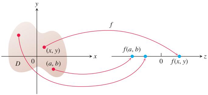
FIGURE 13.1 An arrow diagram for the function
As usual, we evaluate functions defined by formulas by substituting the values of the independent variables in the formula and calculating the corresponding value of the dependent variable. For example, the value of
Domains and Ranges
In defining a function of more than one variable, we follow the usual practice of excluding inputs that lead to complex numbers or division by zero. If
EXAMPLE 1
(a) These are functions of two variables. Note the restrictions that apply to their domains in order to obtain a real value for the dependent variable z.
| Function | Domain | Range |
| Entire plane |
(b) These are functions of three variables with restrictions on some of their domains.
| Function | Domain | Range |
| Entire space | ||
| Half-space |
Functions of Two Variables
On the real line, closed intervals
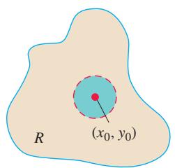
(a) Interior point
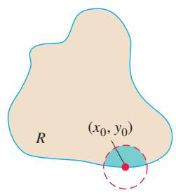
FIGURE 13.2 Interior points and boundary points of a plane region R. An interior point is necessarily a point of R. A boundary point of R need not belong to R.
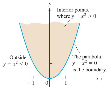
FIGURE 13.4 The domain of
DEFINITIONS A point
in a region (set) R in the xy-plane is an interior point of R if it is the center of a disk of positive radius that lies entirely in R (Figure 13.2). A point ( 𝑥 0 , 𝑦 0 ) is a boundary point of R if every disk centered at ( 𝑥 0 , 𝑦 0 ) contains points that lie outside of R as well as points that lie in R. (The boundary point itself need not belong to R.) ( 𝑥 0 , 𝑦 0 )
The interior points of a region, as a set, make up the interior of the region. The region’s boundary points make up its boundary. A region is open if it consists entirely of interior points. A region is closed if it contains all its boundary points (Figure 13.3).
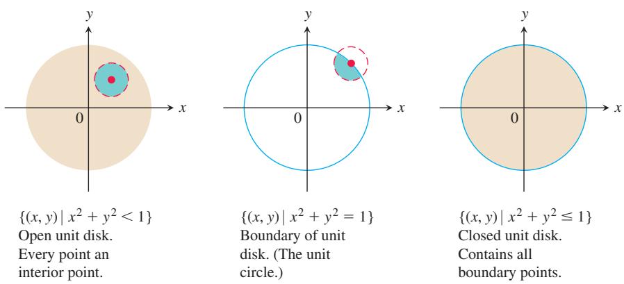
FIGURE 13.3 Interior points and boundary points of the unit disk in the plane.
As with a half-open interval of real numbers [ )a b, , some regions in the plane are neither open nor closed. If you start with the open disk in Figure 13.3 and add to it some, but not all, of its boundary points, the resulting set is neither open nor closed. The boundary points that are there keep the set from being open. The absence of the remaining boundary points keeps the set from being closed. Two interesting examples are the empty set and the entire plane. The empty set has no interior points and no boundary points. This implies that the empty set is open (because it does not contain points that are not interior points), and at the same time it is closed (because there are no boundary points that it fails to contain). The entire xy-plane is also both open and closed: open because every point in the plane is an interior point, and closed because it has no boundary points. The empty set and the entire plane are the only subsets of the plane that are both open and closed. Other sets may be open, or closed, or neither.
DEFINITIONS A region in the plane is bounded if it lies inside a disk of finite radius. A region is unbounded if it is not bounded.
Examples of bounded sets in the plane include line segments, triangles, interiors of triangles, rectangles, circles, and disks. Examples of unbounded sets in the plane include lines, coordinate axes, the graphs of functions defined on infinite intervals, quadrants, halfplanes, and the plane itself.
EXAMPLE 2 Describe the domain of the function
Solution Since f is defined only where
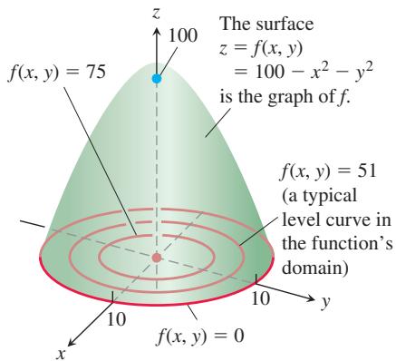
FIGURE 13.5 The graph and selected level curves of the function
The contour curve
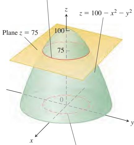
The level curve
FIGURE 13.6 A plane z = c parallel to the xy-plane intersecting a surface
Graphs, Level Curves, and Contours of Functions of Two Variables
There are two standard ways to picture the values of a function
DEFINITIONS The set of points in the plane where a function
has a constant value 𝑓 ( 𝑥 , 𝑦 ) is called a level curve of 𝑓 ( 𝑥 , 𝑦 ) = 𝑐 The set of all points 𝑓 . in space, for ( 𝑥 , 𝑦 , 𝑓 ( 𝑥 , 𝑦 ) ) in the domain of ( 𝑥 , 𝑦 ) is called the graph of 𝑓 , 𝑓 .
The graph of f is often called the surface
EXAMPLE 3 Graph
Solution The domain of f is the entire xy-plane, and the range of f is the set of real numbers less than or equal to 100. The graph is the paraboloid
The level curve
which is the circle of radius 10 centered at the origin. Similarly, the level curves
The level curve
The curve in space in which the plane
The distinction between level curves and contour curves is often overlooked, and it is common to call both types of curves by the same name, relying on context to make it clear which type of curve is meant. On most maps, for example, the curves that represent constant elevation (height above sea level) are called contours, not level curves (Figure 13.7).
Functions of Three Variables
In the plane, the points where a function of two independent variables has a constant value
DEFINITION The set of points
in space where a function of three independent variables has a constant value ( 𝑥 , 𝑦 , 𝑧 ) is called a level surface of 𝑓 ( 𝑥 , 𝑦 , 𝑧 ) = 𝑐 𝑓 .
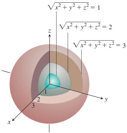
FIGURE 13.8 The level surfaces of
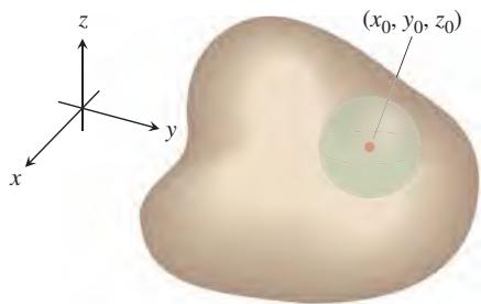
(a) Interior point
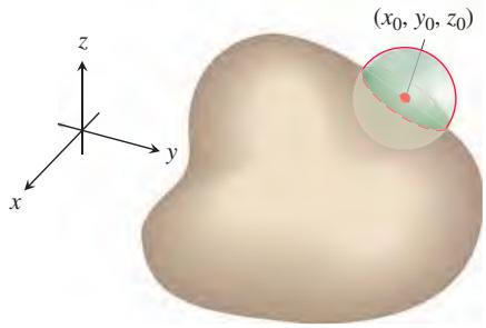
(b) Boundary point
FIGURE 13.9 Interior points and boundary points of a region in space. As with regions in the plane, a boundary point need not belong to the space region R.
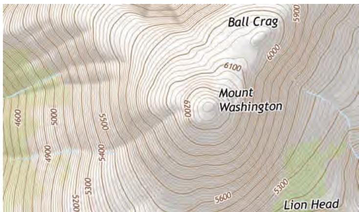
FIGURE 13.7 Contours on Mt. Washington in New Hampshire. (Source: United States Geological Survey)
Since the graphs of functions of three variables consist of points
EXAMPLE 4 Describe the level surfaces of the function
Solution The value of f is the distance from the origin to the point
We are not graphing the function here; we are looking at level surfaces in the function’sdomain. The level surfaces show how the function’s values change as we move through itsdomain. If we remain on a sphere of radius c centered at the origin, the function maintains aconstant value, namely c. If we move from a point on one sphere to a point on another, thefunction’s value changes. It increases if we move away from the origin and decreases if wemove toward the origin. The way the values change depends on the direction we take. Thedependence of change on direction is important. We return to it in Section 13.5. 一
The definitions of interior, boundary, open, closed, bounded, and unbounded for regions in space are similar to those for regions in the plane. To accommodate the extra dimension, we use solid balls of positive radius instead of disks.
DEFINITIONS A point
in a region R in space is an interior point of R if it is the center of a solid ball that lies entirely in R (Figure 13.9a). A point ( 𝑥 0 , 𝑦 0 , 𝑧 0 ) is a boundary point of R if every solid ball centered at ( 𝑥 0 , 𝑦 0 , 𝑧 0 ) contains points that lie outside of R as well as points that lie inside R (Figure 13.9b). The interior of R is the set of interior points of R. The boundary of R is the set of boundary points of R. ( 𝑥 0 , 𝑦 0 , 𝑧 0 )
A region is open if it consists entirely of interior points. A region is closed if it contains its entire boundary.
A region is bounded if it lies inside a solid ball of finite radius; otherwise, the region is unbounded.
Examples of open sets in space include the interior of a sphere, the open half-space
Functions of more than three independent variables are also important. For example, a model that measures temperature in the atmosphere may depend not only on the location of the point
Computer Graphing
Three-dimensional graphing software makes it possible to graph functions of two variables. We can often get information more quickly from a graph than from a formula, since the surfaces reveal increasing and decreasing behavior, and high points or low points.
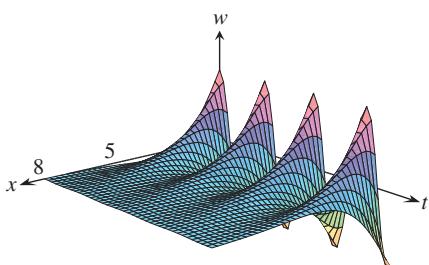
EXAMPLE 5 The temperature w beneath the Earth’s surface is a function of the depth x beneath the surface and the time t of the year. If we measure x in meters and t as the number of days elapsed from the expected date of the yearly highest surface temperature, we can model the variation in temperature with the function
FIGURE 13.10 This graph shows the seasonal variation of the temperature below ground as a fraction of surface temperature (Example 5).
(The temperature at 0 m is scaled to vary from +1 to −1, so that the variation at x meters can be interpreted as a fraction of the variation at the surface.)
Figure 13.10 shows a graph of the function. At a depth of 5 m, the variation (change in vertical amplitude in the figure) is about 5% of the surface variation. At 8 m, there is almost no variation during the year.
The graph also shows that the temperature 5 m below the surface is about half a yearout of phase with the surface temperature. When the temperature is lowest on the surface(late January, say), it is at its highest 5 m below. Five meters below the ground, the seasonsare reversed. 一
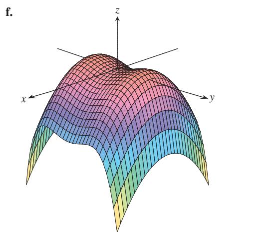
Figure 13.11 shows computer-generated graphs of a number of functions of two variables together with their level curves.
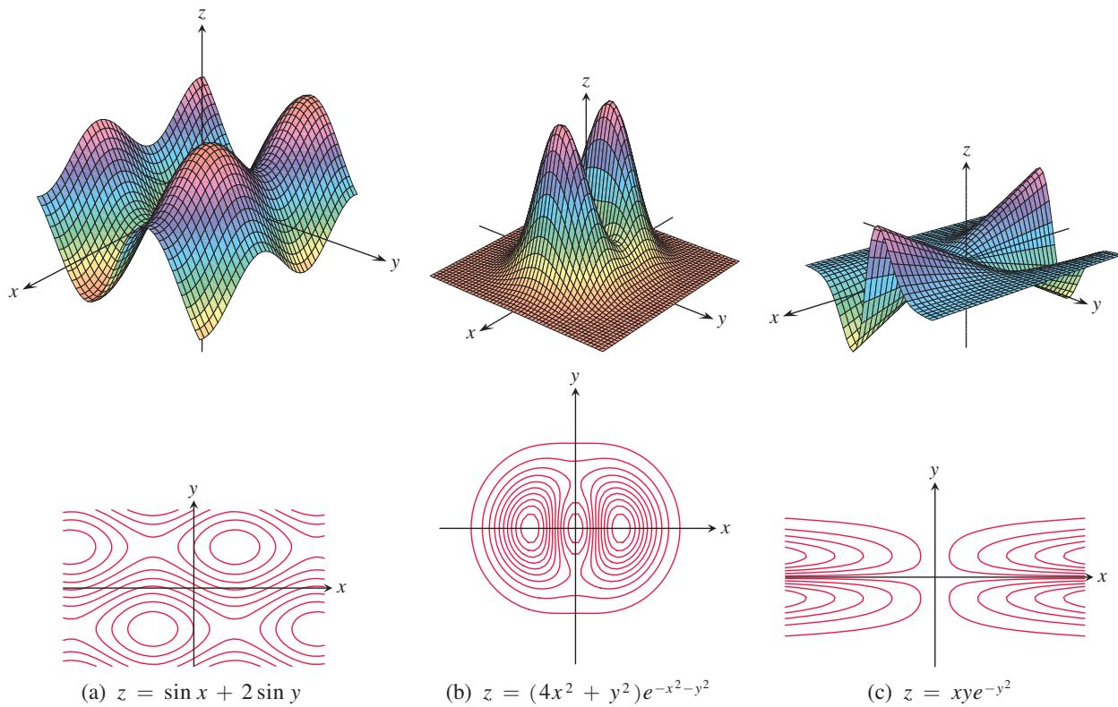
FIGURE 13.11 Computer-generated graphs and level curves of typical functions of two variables.
Exercises 13.1
Domain, Range, and Level Curves
In Exercises 1–4, find the specific function values. 1.
-
𝑓 ( 𝑥 , 𝑦 ) = s i n ( 𝑥 𝑦 ) 𝑓 ( 2 , 𝜋 6 ) 𝑓 ( − 3 , 𝜋 1 2 ) 𝑓 ( 𝜋 , 1 4 ) 𝑓 ( − 𝜋 2 , − 7 ) -
𝑓 ( 𝑥 , 𝑦 , 𝑧 ) = 𝑥 − 𝑦 𝑦 2 + 𝑧 2 𝑓 ( 3 , − 1 , 2 ) 𝑓 ( 1 , 1 2 , − 1 4 ) 𝑓 ( 0 , − 1 3 , 0 ) 𝑓 ( 2 , 2 , 1 0 0 ) -
𝑓 ( 𝑥 , 𝑦 , 𝑧 ) = √ 4 9 − 𝑥 2 − 𝑦 2 − 𝑧 2 𝑓 ( 0 , 0 , 0 ) 𝑓 ( 2 , − 3 , 6 ) 𝑓 ( − 1 , 2 , 3 ) 𝑓 ( 4 √ 2 , 5 √ 2 , 6 √ 2 )
In Exercises 5–12, find and sketch the domain for each function.
-
𝑓 ( 𝑥 , 𝑦 ) = √ 𝑦 − 𝑥 − 2 -
𝑓 ( 𝑥 , 𝑦 ) = l n ( 𝑥 2 + 𝑦 2 − 4 ) -
𝑓 ( 𝑥 , 𝑦 ) = ( 𝑥 − 1 ) ( 𝑦 + 2 ) ( 𝑦 − 𝑥 ) ( 𝑦 − 𝑥 3 ) -
𝑓 ( 𝑥 , 𝑦 ) = s i n ( 𝑥 𝑦 ) 𝑥 2 + 𝑦 2 − 2 5 -
𝑓 ( 𝑥 , 𝑦 ) = c o s − 1 ( 𝑦 − 𝑥 2 ) -
𝑓 ( 𝑥 , 𝑦 ) = l n ( 𝑥 𝑦 + 𝑥 − 𝑦 − 1 ) -
𝑓 ( 𝑥 , 𝑦 ) = √ ( 𝑥 2 − 4 ) ( 𝑦 2 − 9 ) -
𝑓 ( 𝑥 , 𝑦 ) = 1 l n ( 4 − 𝑥 2 − 𝑦 2 )
In Exercises 13–16, find and sketch the level curves
-
𝑓 ( 𝑥 , 𝑦 ) = 𝑥 + 𝑦 − 1 , 𝑐 = − 3 , − 2 , − 1 , 0 , 1 , 2 , 3 -
𝑓 ( 𝑥 , 𝑦 ) = 𝑥 2 + 𝑦 2 , 𝑐 = 0 , 1 , 4 , 9 , 1 6 , 2 5 -
𝑓 ( 𝑥 , 𝑦 ) = 𝑥 𝑦 , 𝑐 = − 9 , − 4 , − 1 , 0 , 1 , 4 , 9 -
𝑓 ( 𝑥 , 𝑦 ) = √ 2 5 − 𝑥 2 − 𝑦 2 , 𝑐 = 0 , 1 , 2 , 3 , 4
In Exercises 17–30, (a) find the function’s domain, (b) find the function’s range, (c) describe the function’s level curves, (d) find the boundary of the function’s domain, (e) determine whether the domain is an open region, a closed region, or neither, and (f) decide whether the domain is bounded or unbounded.
-
𝑓 ( 𝑥 , 𝑦 ) = 𝑦 − 𝑥 -
𝑓 ( 𝑥 , 𝑦 ) = √ 𝑦 − 𝑥 -
𝑓 ( 𝑥 , 𝑦 ) = 4 𝑥 2 + 9 𝑦 2 -
𝑓 ( 𝑥 , 𝑦 ) = 𝑥 2 − 𝑦 2 -
𝑓 ( 𝑥 , 𝑦 ) = 𝑥 𝑦 -
𝑓 ( 𝑥 , 𝑦 ) = 𝑦 / 𝑥 2 -
𝑓 ( 𝑥 , 𝑦 ) = 1 √ 1 6 − 𝑥 2 − 𝑦 2 -
𝑓 ( 𝑥 , 𝑦 ) = √ 9 − 𝑥 2 − 𝑦 2 -
𝑓 ( 𝑥 , 𝑦 ) = l n ( 𝑥 2 + 𝑦 2 ) -
𝑓 ( 𝑥 , 𝑦 ) = 𝑒 − ( 𝑥 2 + 𝑦 2 ) -
𝑓 ( 𝑥 , 𝑦 ) = s i n − 1 ( 𝑦 − 𝑥 ) -
𝑓 ( 𝑥 , 𝑦 ) = t a n − 1 ( 𝑦 𝑥 ) -
𝑓 ( 𝑥 , 𝑦 ) = l n ( 𝑥 2 + 𝑦 2 − 1 ) -
f ( ) x y x y , ln 9 = − − ( ) 2 2
Matching Surfaces with Level Curves
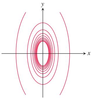
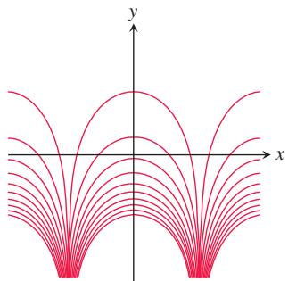
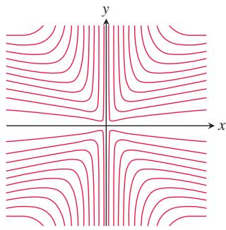
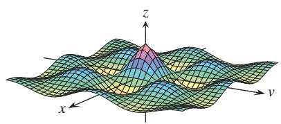
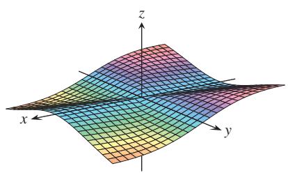
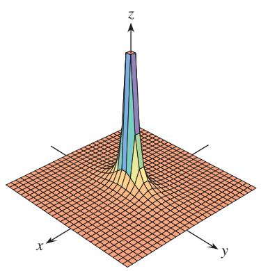
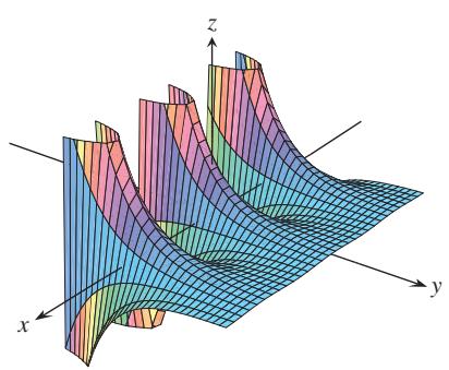
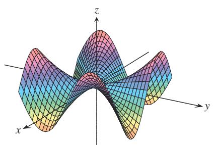
Exercises 31–36 show level curves for six functions. The graphs of these functions are given on the next page (items a–f ), as are their equations (items g–l). Match each set of level curves with the appropriate graph and the appropriate equation.
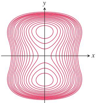
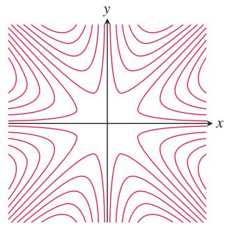
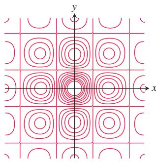
a.
b.
c.
d.
e.
xy2 g. =z h. z = − − y y x 2 4 2 +x y2 2
i. = ( )( ) − + z cos cosx y e x y 4 2 2
l.
Functions of Two Variables
Display the values of the functions in Exercises 37–48 in two ways: (a) by sketching the surface
-
𝑓 ( 𝑥 , 𝑦 ) = 𝑦 2 -
𝑓 ( 𝑥 , 𝑦 ) = 𝑥 2 + 𝑦 2
Finding Level Curves
-
𝑓 ( 𝑥 , 𝑦 ) = √ 𝑥 2 + 𝑦 2 -
𝑓 ( 𝑥 , 𝑦 ) = 𝑥 2 − 𝑦 -
𝑓 ( 𝑥 , 𝑦 ) = 4 − 𝑥 2 − 𝑦 2 -
𝑓 ( 𝑥 , 𝑦 ) = 4 𝑥 2 + 𝑦 2 -
𝑓 ( 𝑥 , 𝑦 ) = 6 − 2 𝑥 − 3 𝑦 -
𝑓 ( 𝑥 , 𝑦 ) = 1 − | 𝑦 | -
𝑓 ( 𝑥 , 𝑦 ) = 1 − | 𝑥 | − | 𝑦 |
𝑓 ( 𝑥 , 𝑦 ) = √ 𝑥 2 + 𝑦 2 + 4
In Exercises 49–52, find an equation for, and sketch the graph of, the level curve of the function
-
𝑓 ( 𝑥 , 𝑦 ) = 1 6 − 𝑥 2 − 𝑦 2 , ( 2 √ 2 , √ 2 ) -
𝑓 ( 𝑥 , 𝑦 ) = √ 𝑥 2 − 1 , ( 1 , 0 ) -
𝑓 ( 𝑥 , 𝑦 ) = √ 𝑥 + 𝑦 2 − 3 , ( 3 , − 1 ) -
𝑓 ( 𝑥 , 𝑦 ) = 2 𝑦 − 𝑥 𝑥 + 𝑦 + 1 , ( − 1 , 1 )
Sketching Level Surfaces
In Exercises 53–60, sketch a typical level surface for the function.
-
f ( ) x y z z , , =
-
𝑓 ( 𝑥 , 𝑦 , 𝑧 ) = 𝑥 2 + 𝑦 2 -
𝑓 ( 𝑥 , 𝑦 , 𝑧 ) = 𝑧 − 𝑥 2 − 𝑦 2
- f ( ) ( ) ( ) ( ) x y z x y z , , 25 16 9 = + + 2 2 2
Finding Level Surfaces
In Exercises 61–64, find an equation for the level surface of the function through the given point.
𝑔 ( 𝑥 , 𝑦 , 𝑧 ) = 𝑥 − 𝑦 + 𝑧 2 𝑥 + 𝑦 − 𝑧 , ( 1 , 0 , − 2 )
In Exercises 65–68, find and sketch the domain of
-
𝑓 ( 𝑥 , 𝑦 ) = ∑ ∞ 𝑛 = 0 ( 𝑥 𝑦 ) 𝑛 , ( 1 , 2 ) -
𝑔 ( 𝑥 , 𝑦 , 𝑧 ) = ∑ ∞ 𝑛 = 0 ( 𝑥 + 𝑦 ) 𝑛 𝑛 ! 𝑧 𝑛 , ( l n 4 , l n 9 , 2 ) -
𝑓 ( 𝑥 , 𝑦 ) = ∫ 𝑦 𝑥 𝑑 𝜃 √ 1 − 𝜃 2 , ( 0 , 1 ) -
𝑔 ( 𝑥 , 𝑦 , 𝑧 ) = ∫ 𝑦 𝑥 𝑑 𝑡 1 + 𝑡 2 + ∫ 𝑧 0 𝑑 𝜃 √ 4 − 𝜃 2 , ( 0 , 1 , √ 3 )
COMPUTER EXPLORATIONS
Use a CAS to perform the following steps for each of the functions in Exercises 69–72.
a. Plot the surface over the given rectangle.
b. Plot several level curves in the rectangle.
c. Plot the level curve of f through the given point.
-
𝑓 ( 𝑥 , 𝑦 ) = 𝑥 s i n 𝑦 2 + 𝑦 0 ≤ 𝑥 ≤ 5 𝜋 , 0 ≤ 𝑦 ≤ 5 𝜋 , -
𝑓 ( 𝑥 , 𝑦 ) = ( s i n 𝑥 ) ( c o s 𝑦 ) 𝑒 √ 𝑥 2 + 𝑦 2 / 8 , 0 ≤ 𝑥 ≤ 5 𝜋 ,
-
𝑓 ( 𝑥 , 𝑦 ) = s i n ( 𝑥 + 2 c o s 𝑦 ) , − 2 𝜋 ≤ 𝑥 ≤ 2 𝜋 , -
𝑓 ( 𝑥 , 𝑦 ) = 𝑒 ( 𝑥 0 . 1 − 𝑦 ) s i n ( 𝑥 2 + 𝑦 2 ) , 0 ≤ 𝑥 ≤ 2 𝜋 , − 2 𝜋 ≤ 𝑦 ≤ 𝜋 , 𝑃 ( 𝜋 , − 𝜋 )
Use a CAS to plot the implicitly defined level surfaces in Exercises
-
4 ln
𝜓 1 ( 𝑥 2 + 𝑦 2 + 𝑧 2 ) = 1 7 4 , 𝑥 2 + 𝑧 2 = 1 -
𝑥 + 𝑦 2 − 3 𝑧 2 = 1 -
s
l n ( 𝑥 2 ) − ( c o s 𝑦 ) √ 𝑥 2 + 𝑧 2 = 2
Parametrized Surfaces Just as you describe curves in the plane parametrically with a pair of equations
𝑥 = 𝑢 c o s 𝑣 , 𝑦 = 𝑢 s i n 𝑣 , 𝑧 = 𝑢 , 0 ≤ 𝑢 ≤ 2 ,
-
x = + = + = ( ) ( ) 2 cos cos , 2 cos sin , sin ,u y u z u υ υ
0 ≤ 𝑢 ≤ 2 𝜋 , 0 ≤ 𝑣 ≤ 2 𝜋 -
𝑥 = 2 c o s 𝑢 c o s 𝑣 , 𝑦 = 2
13.2 Limits and Continuity in Higher Dimensions
In this section we develop limits and continuity for multivariable functions. The theory is similar to that developed for single-variable functions, but since we now have more than one independent variable, there is additional complexity that requires some new ideas.
Limits for Functions of Two Variables
If the values of
DEFINITION Suppose that every open circular disk centered at
contains a point in the domain of ( 𝑥 0 , 𝑦 0 ) other than 𝑓 itself. We say that a function ( 𝑥 0 , 𝑦 0 ) approaches the limit L as 𝑓 ( 𝑥 , 𝑦 ) approaches ( 𝑥 , 𝑦 ) , and write ( 𝑥 0 , 𝑦 0 ) l i m ( 𝑥 , 𝑦 ) → ( 𝑥 0 , 𝑦 0 ) 𝑓 ( 𝑥 , 𝑦 ) = 𝐿 , if, for every number
, there exists a corresponding number 𝜀 > 0 . such that for all 𝛿 > 0 in the domain of ( 𝑥 , 𝑦 ) 𝑓 , | 𝑓 ( 𝑥 , 𝑦 ) − 𝐿 | < 𝜀 w h e n e v e r 0 < √ ( 𝑥 − 𝑥 0 ) 2 + ( 𝑦 − 𝑦 0 ) 2 < 𝛿 .
The definition of limit says that the distance between
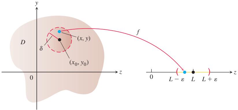
FIGURE 13.12 In the limit definition, δ is the radius of a disk centered at
As for functions of a single variable, it can be shown that
For example, in the first limit statement above,
then
That is,
So a δ has been found satisfying the requirement of the definition, and therefore we have proved that
Equation (1) is a special case of the more general formula
according to which, if
following formula generalizes Equation (2):
As with single-variable functions, the limit of the sum of two functions is the sum of their limits (when they both exist), with similar results for the limits of the differences, constant multiples, products, quotients, powers, and roots. These facts are summarized in Theorem 1.
THEOREM 1—Properties of Limits of Functions of Two Variables
The following rules hold if L, M, and k are real numbers and
- Sum Rule:
- Difference Rule:
- Constant Multiple Rule:
- Product Rule:
- Quotient Rule:
- Power Rule:
- Root Rule:
n a positive integer, and if n is even,
- Composition Rule:
Although we will not prove Theorem 1 here, we give an informal discussion of why it is true. If
When we apply Theorem 1 and Equations (1)–(3) to polynomials and rational functions, we obtain the useful result that the limits of these functions as
EXAMPLE 1 In this example, we combine Equations (1)–(5) with the results in Theorem 1 to calculate the limits.
(a)
Solution Since the denominator
We can cancel the factor
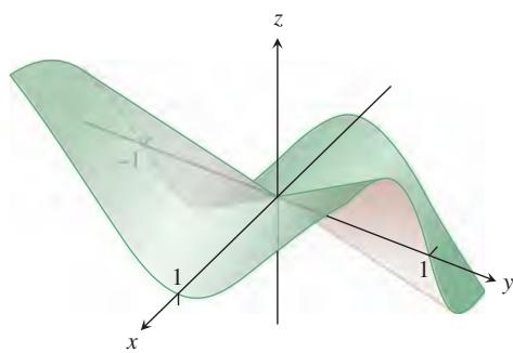
FIGURE 13.13 The surface graph suggests that the limit of the function in Example 3 must be 0, if it exists.
EXAMPLE 3
Solution We first observe that along the line
Let
or
Since
So if we choose
It follows from the definition that
(a)
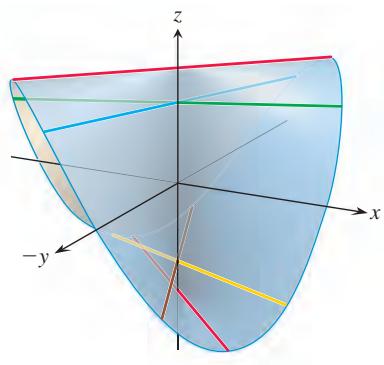
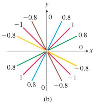
FIGURE 13.14 (a) The graph of
The function is continuous at every point except the origin. (b) The value of
EXAMPLE 4
Solution The domain of
Continuity
As with functions of a single variable, continuity is defined in terms of limits.
DEFINITION Suppose that every open circular disk centered at
contains a point in the domain of ( 𝑥 0 , 𝑦 0 ) other than 𝑓 itself. Then a function ( 𝑥 0 , 𝑦 0 ) is continuous at the point 𝑓 ( 𝑥 , 𝑦 ) if ( 𝑥 0 , 𝑦 0 )
is defined at 𝑓 9 ( 𝑥 0 , 𝑦 0 )
exists, and l i m ( 𝑥 , 𝑦 ) → ( 𝑥 0 , 𝑦 0 ) 𝑓 ( 𝑥 , 𝑦 ) l i m ( 𝑥 , 𝑦 ) → ( 𝑥 0 , 𝑦 0 ) 𝑓 ( 𝑥 , 𝑦 ) = 𝑓 ( 𝑥 0 , 𝑦 0 ) .
A function is continuous if it is continuous at every point of its domain.
As with the definition of limit, the definition of continuity applies at boundary points as well as interior points of the domain of
A consequence of Theorem 1 is that algebraic combinations of continuous functions are continuous at every point at which all the functions involved are defined. This means that sums, differences, constant multiples, products, quotients, and powers of continuous functions are continuous where defined. In particular, polynomials and rational functions of two variables are continuous at every point at which they are defined.
EXAMPLE 5 Show that
is continuous at every point except the origin (Figure 13.14).
Solution The function
(a)
(b)
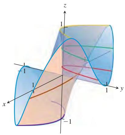
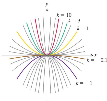
FIGURE 13.15 (a) The graph of
For every value of
Therefore,
This limit changes with each value of the slope m. There is therefore no single number wemay call the limit of
Examples 4 and 5 illustrate an important point about limits of functions of two or more variables. For a limit to exist at a point, the limit must be the same along every approach path. This result is analogous to the single-variable case where both the left- and right-sided limits had to have the same value. For functions of two or more variables, if we ever find paths with different limits, we know the function has no limit at the point they approach.
Two-Path Test for Nonexistence of a Limit
If a function
EXAMPLE 6 Show that the function
(Figure 13.15) has no limit as
Solution As
Therefore,
This limit varies with the path of approach. If
It can be shown that the function in Example 6 has limit 0 along every straight line path
Having the same limit along all straight lines approaching
Whenever it is correctly defined, the composition of continuous functions is also continuous. The only requirement is that each function be continuous where it is applied. The proof, omitted here, is similar to that for functions of a single variable (Theorem 9 in Section 2.6).
Continuity of Compositions
If
For example, the composite functions
are continuous at every point
Functions of More Than Two Variables
The definitions of limit and continuity for functions of two variables and the conclusions about limits and continuity for sums, products, quotients, powers, and compositions all extend to functions of three or more variables. Functions like
are continuous throughout their domains, and limits like
where P denotes the point
Extreme Values of Continuous Functions on Closed, Bounded Sets
The Extreme Value Theorem (Theorem 1, Section 4.1) states that a function of a single variable that is continuous at every point of a closed, bounded interval
Similar results hold for functions of three or more variables. A continuous function
EXERCISES
Limits with Two Variables
Find the limits in Exercises 1–12.
-
l i m ( 𝑥 , 𝑦 ) → ( 0 , l n 2 ) 𝑒 𝑥 − 𝑦 -
l i m ( 𝑥 , 𝑦 ) ( 1 , 1 ) l n | 1 + 𝑥 2 𝑦 2 | -
l i m ( 𝑥 , 𝑦 ) → ( 0 , 0 ) 𝑒 𝑦 s i n 𝑥 𝑥 -
l i m ( 𝑥 , 𝑦 ) → ( 1 / 2 7 , 𝜋 3 ) c o s 3 √ 𝑥 𝑦 -
l i m ( 𝑥 , 𝑦 ) → ( 1 , 𝜋 / 6 ) 𝑥 s i n 𝑦 𝑥 2 + 1 -
l i m ( 𝑥 , 𝑦 ) → ( 𝜋 / 2 , 0 ) c o s 𝑦 + 1 𝑦 − s i n 𝑥
Limits of Quotients
Find the limits in Exercises 13–24 by rewriting the fractions first.
-
l i m ( 𝑥 , 𝑦 ) → ( 1 , 1 ) 𝑥 2 − 2 𝑥 𝑦 + 𝑦 2 𝑥 − 𝑦 -
l i m ( 𝑥 , 𝑦 ) → ( 1 , 1 ) 𝑥 ≠ 𝑦 𝑥 2 − 𝑦 2 𝑥 − 𝑦 -
l i m ( 𝑥 , 𝑦 ) → ( 1 , 1 ) 𝑥 𝑦 − 𝑦 − 2 𝑥 + 2 𝑥 − 1 -
l i m ( 𝑥 , 𝑦 ) → ( 2 , − 4 ) 𝑦 + 4 𝑥 2 𝑦 − 𝑥 𝑦 + 4 𝑥 2 − 4 𝑥 -
l i m ( 𝑥 , 𝑦 ) → ( 0 , 0 ) 𝑥 − 𝑦 + 2 √ 𝑥 − 2 √ 𝑦 √ 𝑥 − √ 𝑦 -
l i m ( 𝑥 , 𝑦 ) → ( 2 , 2 ) 𝑥 + 𝑦 − 4 √ 𝑥 + 𝑦 − 2 -
l i m ( 𝑥 , 𝑦 ) → ( 2 , 0 ) √ 2 𝑥 − 𝑦 − 2 2 𝑥 − 𝑦 − 4 -
l i m ( 𝑥 , 𝑦 ) → ( 4 , 3 ) √ 𝑥 − √ 𝑦 + 1 𝑥 − 𝑦 − 1 -
l i m ( 𝑥 , 𝑦 ) ( 0 , 0 ) s i n ( 𝑥 2 + 𝑦 2 ) 𝑥 2 + 𝑦 2 -
l i m ( 𝑥 , 𝑦 ) ( 0 , 0 ) 1 − c o s ( 𝑥 𝑦 ) 𝑥 𝑦 -
l i m ( 𝑥 , 𝑦 ) ( 1 , − 1 ) 𝑥 3 + 𝑦 3 𝑥 + 𝑦 -
l i m ( 𝑥 , 𝑦 ) → ( 2 , 2 ) 𝑥 − 𝑦 𝑥 4 − 𝑦 4
Limits with Three Variables
Find the limits in Exercises 25–30.
-
l i m → ( 1 , 3 , 4 ) ( 1 𝑥 + 1 𝑦 + 1 𝑧 ) -
l i m 𝑃 → ( 1 , − 1 , − 1 ) 2 𝑥 𝑦 + 𝑦 𝑧 𝑥 2 + 𝑧 2 -
l i m 𝑃 → ( 𝜋 , 𝜋 , 0 ) ( s i n 2 𝑥 + c o s 2 𝑦 + s e c 2 𝑧 ) -
l i m 𝑃 → ( − 1 / 4 , 𝜋 / 2 , 2 ) t a n − 1 𝑥 𝑦 𝑧 -
l i m 𝑃 → ( 𝜋 , 0 , 3 ) 𝑧 𝑒 − 2 𝑦 c o s 2 𝑥 -
l i m 𝑃 → ( 2 , − 3 , 6 ) l n √ 𝑥 2 + 𝑦 2 + 𝑧 2
Continuity for Two Variables
At what points (x y, in the plane are the functions in Exercises 31–34) continuous?
-
a.
𝑓 ( 𝑥 , 𝑦 ) = s i n ( 𝑥 + 𝑦 ) 𝑓 ( 𝑥 , 𝑦 ) = l n ( 𝑥 2 + 𝑦 2 ) -
a.
𝑓 ( 𝑥 , 𝑦 ) = 𝑥 + 𝑦 𝑥 − 𝑦
b.
b.
- a.
𝑔 ( 𝑥 , 𝑦 ) = 𝑥 2 + 𝑦 2 𝑥 2 − 3 𝑥 + 2 𝐛 . 𝑔 ( 𝑥 , 𝑦 ) = 1 𝑥 2 − 𝑦
Continuity for Three Variables
At what points ( x y z , , in space are the functions in Exercises 35–40) continuous?
- a.
𝑓 ( 𝑥 , 𝑦 , 𝑧 ) = 𝑥 2 + 𝑦 2 − 2 𝑧 2
b.
-
a.
𝑓 ( 𝑥 , 𝑦 , 𝑧 ) = l n 𝑥 𝑦 𝑧 𝑓 ( 𝑥 , 𝑦 , 𝑧 ) = 𝑒 𝑥 + 𝑦 c o s 𝑧 -
a.
ℎ ( 𝑥 , 𝑦 , 𝑧 ) = 𝑥 𝑦 s i n 1 𝑧 ℎ ( 𝑥 , 𝑦 , 𝑧 ) = 1 𝑥 2 + 𝑧 2 − 1 -
a.
ℎ ( 𝑥 , 𝑦 , 𝑧 ) = 1 | 𝑦 | + | 𝑧 | ℎ ( 𝑥 , 𝑦 , 𝑧 ) = 1 | 𝑥 𝑦 | + | 𝑧 | -
a.
ℎ ( 𝑥 , 𝑦 , 𝑧 ) = l n ( 𝑧 − 𝑥 2 − 𝑦 2 − 1 )
b.
- a.
ℎ ( 𝑥 , 𝑦 , 𝑧 ) = √ 4 − 𝑥 2 − 𝑦 2 − 𝑧 2
b.
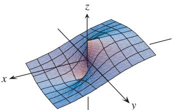
No Limit Exists at the Origin
By considering different paths of approach, show that the functions in Exercises 41–48 have no limit as
-
𝑓 ( 𝑥 , 𝑦 ) = − 𝑥 √ 𝑥 2 + 𝑦 2 -
𝑓 ( 𝑥 , 𝑦 ) = 𝑥 4 𝑥 4 + 𝑦 2
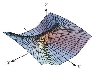
-
𝑓 ( 𝑥 , 𝑦 ) = 𝑥 4 − 𝑦 2 𝑥 4 + 𝑦 2 -
𝑓 ( 𝑥 , 𝑦 ) = 𝑥 𝑦 | 𝑥 𝑦 | -
𝑔 ( 𝑥 , 𝑦 ) = 𝑥 − 𝑦 𝑥 + 𝑦 -
𝑔 ( 𝑥 , 𝑦 ) = 𝑥 2 − 𝑦 𝑥 − 𝑦 -
ℎ ( 𝑥 , 𝑦 ) = 𝑥 2 + 𝑦 𝑦 -
ℎ ( 𝑥 , 𝑦 ) = 𝑥 2 𝑦 𝑥 4 + 𝑦 2
Theory and Examples
In Exercises 49–54, show that the limits do not exist.
-
l i m ( 𝑥 , 𝑦 ) → ( 1 , 1 ) 𝑥 𝑦 2 − 1 𝑦 − 1 -
l i m ( 𝑥 , 𝑦 ) → ( 0 , 1 ) 𝑥 l n 𝑦 𝑥 2 + ( l n 𝑦 ) 2 -
l i m ( 𝑥 , 𝑦 ) → ( 1 , 0 ) 𝑥 𝑒 𝑦 − 1 𝑥 𝑒 𝑦 − 1 + 𝑦 -
l i m ( 𝑥 , 𝑦 ) → ( 0 , 0 ) 𝑦 + s i n 𝑥 𝑥 + s i n 𝑦
-
l i m ( 𝑥 , 𝑦 ) → ( 1 , 1 ) t a n 𝑦 − 𝑦 t a n 𝑥 𝑦 − 𝑥 -
Let
𝑓 ( 𝑥 , 𝑦 ) = ⎧ { { ⎨ { { ⎩ 1 , 𝑦 ≥ 𝑥 4 1 , 𝑦 ≤ 0 0 , o t h e r w i s
Find each of the following limits, or explain that the limit does not exist.
a.
b.
c.
- Let
𝑓 ( 𝑥 , 𝑦 ) = { 𝑥 2 , 𝑥 ≥ 0 𝑥 3 , 𝑥 < 0 .
Find the following limits.
a.
b.
c.
-
Show that the function in Example 6 has limit 0 along every straight line approaching (0, 0 .)
-
If
𝑓 ( 𝑥 0 , 𝑦 0 ) = 3 ,
if f is continuous at
The Sandwich Theorem for functions of two variables states that if
Use this result to support your answers to the questions in Exercises 59–62.
- Does knowing that
tell you anything about
Give reasons for your answer.
- Does knowing that
tell you anything about
Give reasons for your answer.
- Does knowing that
| s i n ( 1 / 𝑥 ) | ≤ 1
Give reasons for your answer.
- Does knowing that co
( 1 / 𝑦 ) ∣ ≤ 1
Give reasons for your answer.
- (Continuation of Example 5.)
a. Reread Example 5. Then substitute m = tan into theθ formula
and simplify the result to show how the value of f varies with the line’s angle of inclination.
b. Use the formula you obtained in part (a) to show that the limit of
- Continuous extension Define
𝑓 ( 0 , 0 )
to be continuous at the origin.
Changing Variables to Polar Coordinates
If you cannot make any headway with
Given
If such an L exists, then
For instance,
To verify the last of these equalities, we need to show that Equation (1) is satisfied with
Since
the implication holds for all r and θ if we take
In contrast,
takes on all values from 0 to 1 regardless of how small r is, so that
In each of these instances, the existence or nonexistence of the limit as
for
In Exercises 65–70, find the limit of
-
𝑓 ( 𝑥 , 𝑦 ) = 𝑥 3 − 𝑥 𝑦 2 𝑥 2 + 𝑦 2 -
𝑓 ( 𝑥 , 𝑦 ) = c o s ( 𝑥 3 − 𝑦 3 𝑥 2 + 𝑦 2 ) -
𝑓 ( 𝑥 , 𝑦 ) = 𝑦 2 𝑥 2 + 𝑦 2 -
𝑓 ( 𝑥 , 𝑦 ) = 2 𝑥 𝑥 2 + 𝑥 + 𝑦 2 -
𝑓 ( 𝑥 , 𝑦 ) = t a n − 1 ( | 𝑥 | + | 𝑦 | 𝑥 2 + 𝑦 2 ) -
𝑓 ( 𝑥 , 𝑦 ) = 𝑥 2 − 𝑦 2 𝑥 2 + 𝑦 2
In Exercises 71 and
-
𝑓 ( 𝑥 , 𝑦 ) = l n ( 3 𝑥 2 − 𝑥 2 𝑦 2 + 3 𝑦 2 𝑥 2 + 𝑦 2 ) -
𝑓 ( 𝑥 , 𝑦 ) = 3 𝑥 2 𝑦 𝑥 2 + 𝑦 2
Using the Limit Definition
Each of Exercises 73–78 gives a function
-
𝑓 ( 𝑥 , 𝑦 ) = 𝑥 2 + 𝑦 2 , 𝜀 = 0 . 0 1 -
𝑓 ( 𝑥 , 𝑦 ) = 𝑦 / ( 𝑥 2 + 1 ) , 𝜀 = 0 . 0 5 -
𝑓 ( 𝑥 , 𝑦 ) = ( 𝑥 + 𝑦 ) / ( 𝑥 2 + 1 ) , 𝜀 = 0 . 0 1
13.3 Partial Derivatives
𝑓 ( 𝑥 , 𝑦 ) = ( 𝑥 + 𝑦 ) / ( 2 + c o s 𝑥 ) , 𝜀 = 0 . 0 2
Each of Exercises 79–82 gives a function
𝑓 ( 𝑥 , 𝑦 , 𝑧 ) = 𝑥 𝑦 𝑧 , 𝑧 = 0 . 0 0 8
-
𝑓 ( 𝑥 , 𝑦 , 𝑧 ) = t a n 2 𝑥 + t a n 2 𝑦 + t a n 2 𝑧 , 𝜀 = 0 . 0 3 -
S h o w t h a t 𝑓 ( 𝑥 , 𝑦 , 𝑧 ) = 𝑥 + 𝑦 − 𝑧 ( 𝑥 0 , 𝑦 0 , 𝑧 0 ) . -
Show that
𝑓 ( 𝑥 , 𝑦 , 𝑧 ) = 𝑥 2 + 𝑦 2 + 𝑧 2
The calculus of several variables is similar to single-variable calculus applied to several variables, one at a time. When we hold all but one of the independent variables of a function constant and differentiate with respect to that one variable, we get a “partial” derivative. This section shows how partial derivatives are defined and interpreted geometrically, and how to calculate them by applying the familiar rules for differentiating functions of a single variable. The idea of differentiability for functions of several variables requires more than the existence of the partial derivatives, because a point can be approached from many different directions. However, we will see that differentiable functions of several variables behave similarly to differentiable single-variable functions. In particular, they are continuous and can be well approximated by linear functions.
Partial Derivatives of a Function of Two Variables
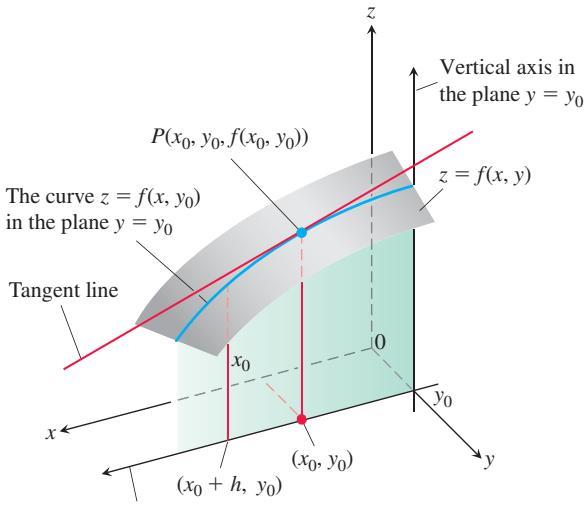
Horizontal axis in the plane
FIGURE 13.16 The intersection of the plane
of the function
We define the partial derivative of f with respect to x at the point
DEFINITION The partial derivative of
with respect to x at the point 𝑓 ( 𝑥 , 𝑦 ) is ( 𝑥 0 , 𝑦 0 ) 𝜕 𝑓 𝜕 𝑥 ∣ ( 𝑥 0 , 𝑦 0 ) = l i m ℎ → 0 𝑓 ( 𝑥 0 + ℎ , 𝑦 0 ) − 𝑓 ( 𝑥 0 , 𝑦 0 ) ℎ , provided the limit exists.
The partial derivative of
A variety of notations are used to denote the partial derivative at a point
When we do not specify a specific point
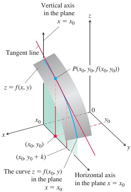
FIGURE 13.17 The intersection of the plane
The slope of the curve
The definition of the partial derivative of
DEFINITION The partial derivative of
with respect to y at the point 𝑓 ( 𝑥 , 𝑦 ) is ( 𝑥 0 , 𝑦 0 ) 𝜕 𝑓 𝜕 𝑦 ∣ ( 𝑥 0 , 𝑦 0 ) = 𝑑 𝑑 𝑦 𝑓 ( 𝑥 0 , 𝑦 ) ∣ 𝑦 = 𝑦 0 = l i m ℎ → 0 𝑓 ( 𝑥 0 , 𝑦 0 + ℎ ) − 𝑓 ( 𝑥 0 , 𝑦 0 ) ℎ ,
The slope of the curve
The partial derivative with respect to y is denoted the same way as the partial derivative with respect to x:
Notice that we now have two tangent lines associated with the surface
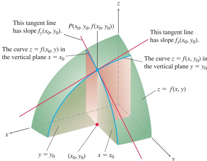
FIGURE 13.18 Figures 13.16 and 13.17 combined. The tangent lines at the point
Calculations
The definitions of
EXAMPLE 1 Find the values of
Solution To find
The value of
To find
The value of
EXAMPLE 2 Find
Solution We treat x as a constant and
EXAMPLE 3 Find
Solution We treat f as a quotient. With y held constant, we use the quotient rule to get
With x held constant and again applying the quotient rule, we get
Implicit differentiation works for partial derivatives the way it works for ordinary derivatives, as the next example illustrates.
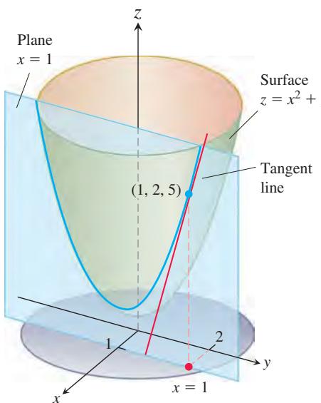
FIGURE 13.19 The tangent line to the curve of intersection of the plane x = 1 and the surface
EXAMPLE 4 Find
defines z as a function of the two independent variables x and
Solution We differentiate both sides of the equation with respect to
EXAMPLE 5 The plane
Solution The parabola lies in a plane parallel to the yz-plane, and the slope is the value of the partial derivative
As a check, we can treat the parabola as the graph of the single-variable function
Functions of More Than Two Variables
The definitions of the partial derivatives of functions of more than two independent variables are similar to the definitions for functions of two variables. They are ordinary derivatives with respect to one variable, taken while the other independent variables are held constant.
EXAMPLE 6
then
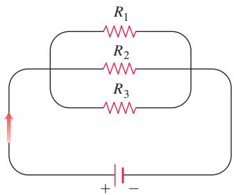
FIGURE 13.20 Resistors arranged this way are said to be connected in parallel (Example 7). Each resistor lets a portion of the current through. Their equivalent resistance R is calculated with the formula
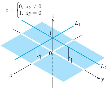
FIGURE 13.21 The graph of
consists of the lines
EXAMPLE 7 If resistors of
(Figure 13.20). Find the value of
Solution To find
When
so
Thus at the given values, a small change in the resistance
Partial Derivatives and Continuity
A function
EXAMPLE 8 Let
(Figure 13.21).
(a) Find the limit of
(b) Find the limit of f as ( x y, approaches ) (0, 0 along the line)
(c) Prove that f is not continuous at the origin.
(d) Show that both partial derivatives
Solution
(a) Since
(b) Since
(c) By the two-path test,
(d) To find
What Example 8 suggests is that we need a stronger requirement for differentiability in higher dimensions than the mere existence of the partial derivatives. We define differentiability for functions of two variables (which is somewhat more complicated than for single-variable functions) at the end of this section and then revisit the connection to continuity.
Second-Order Partial Derivatives
When we differentiate a function
The defining equations are
and so on. Notice the order in which the mixed partial derivatives are taken:
HISTORICAL BIOGRAPHY
Pierre-Simon Laplace
EXAMPLE 9
(1749–1827)
Mathematician and astronomer, Laplace was born in Normandy, France. He was among the most influential scientists of his time and was called the Newton of France for contributions to the understanding of the solar system’s stability. Laplace also generalized the laws of mechanics for their application to the motion and properties of the heavenly bodies.
To know more, visit the companion Website.
Solution The first step is to calculate both first partial derivatives.
Now we find both partial derivatives of each first partial:
The Mixed Derivative Theorem
You may have noticed that the “mixed” second-order partial derivatives
in Example 9 are equal. This is not a coincidence. They must be equal whenever
HISTORICAL BIOGRAPHY
Alexis Clairaut
Alexis Clairaut was a mathematical genius, who was called to visit the Academy of Sciences in Paris when he was only 12 years old. n a study published in 1743, the Clairaut proposition postulates in a simple way the dependency of the geometrical flattening ratio on the relationship between the gravity and the centrifugal force.
To know more, visit the companion Website.
(1713–1765)
THEOREM 2—The Mixed Derivative Theorem If
Theorem 2 is also known as Clairaut’s Theorem, after the French mathematician Alexis Clairaut, who discovered it. A proof is given in Appendix A.10. Theorem 2 says that to calculate a mixed second-order derivative, we may differentiate in either order, provided the continuity conditions are satisfied. This ability to proceed in different order sometimes simplifies our calculations.
EXAMPLE 10 Find
Solution The symbol
If we differentiate first with respect to y, we obtain
Partial Derivatives of Still Higher Order
Although we will deal mostly with first- and second-order partial derivatives, because these appear the most frequently in applications, there is no theoretical limit to how many times we can differentiate a function as long as the derivatives involved exist. Thus, we get third- and fourth-order derivatives denoted by symbols like
and so on. As with second-order derivatives, the order of differentiation is immaterial as long as all the derivatives through the order in question are continuous.
Solution We first differentiate with respect to the variable y, then x, then y again, and finally with respect to z:
Differentiability
The concept of differentiability for functions of several variables is more complicated than for single-variable functions, because a point in the domain can be approached from many directions and along any path, not just from the left or from the right. The existence of both partial derivatives at a point
In Section 3.11, we saw that a differentiable function f can be approximated near a point
This formula allows us to find a linear function
where
where again
Rather than being a consequence of the definition, the differentiability for a function of two variables
and the graph of L is a plane, called the tangent plane, that approximates the graph of f near
We now specify how closely f is approximated by L at
where both
If we insert the formula for
Setting
Based on these ideas, we now state the formal definition of differentiability, which captures the idea that f is well approximated by L.
DEFINITION A function
is differentiable at 𝑧 = 𝑓 ( 𝑥 , 𝑦 ) if both ( 𝑥 0 , 𝑦 0 ) and 𝑓 𝑥 ( 𝑥 0 , 𝑦 0 ) exist and if 𝑓 𝑦 ( 𝑥 0 , 𝑦 0 ) satisfies Δ 𝑧 = 𝑓 ( 𝑥 , 𝑦 ) − 𝑓 ( 𝑥 0 , 𝑦 0 ) Δ 𝑧 = 𝑓 𝑥 ( 𝑥 0 , 𝑦 0 ) Δ 𝑥 + 𝑓 𝑦 ( 𝑥 0 , 𝑦 0 ) Δ 𝑦 + 𝜀 1 Δ 𝑥 + 𝜀 2 Δ 𝑦 , where
, and both Δ 𝑥 = 𝑥 − 𝑥 0 , Δ 𝑦 = 𝑦 − 𝑦 0 , and 𝜀 1 → 0 as 𝜀 2 → 0 . We call the function ( 𝑥 , 𝑦 ) ( 𝑥 0 , 𝑦 0 ) differentiable if it is differentiable at every point in its domain, and we then say that its graph is a smooth surface. 𝑓
The following theorem (proved in Appendix A.10) and its accompanying corollary tell us that functions with continuous first partial derivatives at
THEOREM 3—The Increment Theorem for Functions of Two Variables
Suppose that the first partial derivatives of
[ \Delta z = f(x_{0} + \Delta x, y_{0} + \Delta y) - f(x_{0}, y_{0}) ]
in the value of f that results from moving from
[ \Delta z = f_{x}(x_{0}, y_{0}) \Delta x + f_{y}(x_{0}, y_{0}) \Delta y + \varepsilon_{1} \Delta x + \varepsilon_{2} \Delta y, ]
in which each of
In many cases the partial derivatives are defined and continuous at every point in the domain of
Corollary of Theorem 3
If the partial derivatives
I
THEOREM 4—Differentiable Implies Continuous
If a function
As we can see from Corollary 3 and Theorem 4, a function
EXERCISES
13.3
Calculating First-Order Partial Derivatives
In Exercises 1–22, find
-
𝑓 ( 𝑥 , 𝑦 ) = 2 𝑥 2 − 3 𝑦 − 4 2 . 𝑓 ( 𝑥 , 𝑦 ) = 𝑥 2 − 𝑥 𝑦 + 𝑦 2 -
𝑓 ( 𝑥 , 𝑦 ) = ( 𝑥 2 − 1 ) ( 𝑦 + 2 ) -
f ( ) x y xy x y x y , 5 7 3 6 = − − + − + 2 2 2
-
𝑓 ( 𝑥 , 𝑦 ) = ( 𝑥 𝑦 − 1 ) 2 -
𝑓 ( 𝑥 , 𝑦 ) = ( 2 𝑥 − 3 𝑦 ) 3 -
𝑓 ( 𝑥 , 𝑦 ) = √ 𝑥 2 + 𝑦 2 -
𝑓 ( 𝑥 , 𝑦 ) = ( 𝑥 3 + ( 𝑦 / 2 ) ) 2 / 3 -
𝑓 ( 𝑥 , 𝑦 ) = 1 / ( 𝑥 + 𝑦 ) -
𝑓 ( 𝑥 , 𝑦 ) = 𝑥 / ( 𝑥 2 + 𝑦 2 ) -
𝑓 ( 𝑥 , 𝑦 ) = ( 𝑥 + 𝑦 ) / ( 𝑥 𝑦 − 1 ) -
𝑓 ( 𝑥 , 𝑦 ) = t a n − 1 ( 𝑦 / 𝑥 ) -
𝑓 ( 𝑥 , 𝑦 ) = 𝑒 ( 𝑥 + 𝑦 + 1 ) -
𝑓 ( 𝑥 , 𝑦 ) = 𝑒 − 𝑥 s i n ( 𝑥 + 𝑦 ) -
𝑓 ( 𝑥 , 𝑦 ) = l n ( 𝑥 + 𝑦 ) -
𝑓 ( 𝑥 , 𝑦 ) = 𝑒 𝑥 𝑦 l n 𝑦 -
𝑓 ( 𝑥 , 𝑦 ) = s i n 2 ( 𝑥 − 3 𝑦 ) -
𝑓 ( 𝑥 , 𝑦 ) = c o s 2 ( 3 𝑥 − 𝑦 2 ) -
𝑓 ( 𝑥 , 𝑦 ) = 𝑥 𝑦 -
𝑓 ( 𝑥 , 𝑦 ) = l o g 𝑦 𝑥 -
𝑓 ( 𝑥 , 𝑦 ) = ∫ 𝑦 𝑥 𝑔 ( 𝑡 ) 𝑑 𝑡 -
𝑓 ( 𝑥 , 𝑦 ) = ∑ ∞ 𝑛 = 0 ( 𝑥 𝑦 ) 𝑛 ( | 𝑥 𝑦 | < 1 )
In Exercises 23–34, find
-
f ( ) x y z xy z , , 1 2 = + −2 2
-
f ( ) x y z xy yz xz , , = + +
-
𝑓 ( 𝑥 , 𝑦 , 𝑧 ) = 𝑥 − √ 𝑦 2 + 𝑧 2 -
𝑓 ( 𝑥 , 𝑦 , 𝑧 ) = ( 𝑥 2 + 𝑦 2 + 𝑧 2 ) − 1 / 2 -
𝑓 ( 𝑥 , 𝑦 , 𝑧 ) = a r c s i n ( 𝑥 𝑦 𝑧 ) -
𝑓 ( 𝑥 , 𝑦 , 𝑧 ) = a r c s e c ( 𝑥 + 𝑦 𝑧 ) -
𝑓 ( 𝑥 , 𝑦 , 𝑧 ) = l n ( 𝑥 + 2 𝑦 + 3 𝑧 ) -
𝑓 ( 𝑥 , 𝑦 , 𝑧 ) = 𝑦 𝑧 l n ( 𝑥 𝑦 ) -
𝑓 ( 𝑥 , 𝑦 , 𝑧 ) = 𝑒 − ( 𝑥 2 + 𝑦 2 + 𝑧 2 ) -
𝑓 ( 𝑥 , 𝑦 , 𝑧 ) = 𝑒 − 𝑥 𝑦 𝑧 -
𝑓 ( 𝑥 , 𝑦 , 𝑧 ) = t a n h ( 𝑥 + 2 𝑦 + 3 𝑧 ) -
𝑓 ( 𝑥 , 𝑦 , 𝑧 ) = s i n h ( 𝑥 𝑦 − 𝑧 2 )
In Exercises 35–40, find the partial derivative of the function with respect to each variable.
-
𝑓 ( 𝑡 , 𝛼 ) = c o s ( 2 𝜋 𝑡 − 𝛼 ) -
𝑔 ( 𝑢 , 𝑣 ) = 𝑣 2 𝑒 ( 2 𝑢 / 𝑣 ) -
ℎ ( 𝜌 , 𝜙 , 𝜃 ) = 𝜌 s i n 𝜙 c o s 𝜃 -
𝑔 ( 𝑟 , 𝜃 , 𝑧 ) = 𝑟 ( 1 − c o s 𝜃 ) − 𝑧 -
Work done by the heart (Section 3.11, Exercise 59)
Calculating Second-Order Partial Derivatives
Find all the second-order partial derivatives of the functions in Exercises 41–54.
-
𝑓 ( 𝑥 , 𝑦 ) = 𝑥 + 𝑦 + 𝑥 𝑦 4 2 . 𝑓 ( 𝑥 , 𝑦 ) = s i n 𝑥 𝑦 -
𝑔 ( 𝑥 , 𝑦 ) = 𝑥 2 𝑦 + c o s 𝑦 + 𝑦 s i n 𝑥 -
ℎ ( 𝑥 , 𝑦 ) = 𝑥 𝑒 𝑦 + 𝑦 + 1 -
𝑟 ( 𝑥 , 𝑦 ) = l n ( 𝑥 + 𝑦 ) -
𝑠 ( 𝑥 , 𝑦 ) = a r c t a n ( 𝑦 / 𝑥 ) -
𝑤 = 𝑥 2 t a n ( 𝑥 𝑦 ) -
𝑤 = 𝑦 𝑒 𝑥 2 − 𝑦 -
𝑤 = 𝑥 s i n ( 𝑥 2 𝑦 ) -
𝑤 = 𝑥 − 𝑦 𝑥 2 + 𝑦 -
𝑓 ( 𝑥 , 𝑦 ) = 𝑥 2 𝑦 3 − 𝑥 4 + 𝑦 5 -
𝑔 ( 𝑥 , 𝑦 ) = c o s 𝑥 2 − s i n 3 𝑦 -
𝑧 = 𝑥 s i n ( 2 𝑥 − 𝑦 2 ) -
𝑧 = 𝑥 𝑒 𝑥 / 𝑦 2
Mixed Partial Derivatives
In Exercises 55–60, verify that
-
𝑤 = l n ( 2 𝑥 + 3 𝑦 ) -
𝑤 = 𝑒 𝑥 + 𝑥 l n 𝑦 + 𝑦 -
𝑤 = 𝑥 𝑦 2 + 𝑥 2 𝑦 3 + 𝑥 3 𝑦 4 -
𝑤 = 𝑥 s i n 𝑦 + 𝑦 s i n 𝑥 + 𝑥 𝑦 -
𝑤 = 𝑥 2 𝑦 3 -
𝑤 = 3 𝑥 − 𝑦 𝑥 + 𝑦 -
Which order of differentiation enables one to calculate
𝑓 𝑥 𝑦
a.
b.
c.
e.
f.
- The fifth-order partial derivative
𝜕 5 𝑓 / 𝜕 𝑥 2 𝜕 𝑦 3
a.
b.
c.
d.
Using the Partial Derivative Definition
In Exercises 63–66, use the limit definition of partial derivative to compute the partial derivatives of the functions at the specified points.
-
f x y x y xy , 4 2 3 ,2 ( ) = + − − f∂ and f∂ at 2, 1 ( ) − x∂ y∂
-
𝑓 ( 𝑥 , 𝑦 ) = √ 2 𝑥 + 3 𝑦 − 1 , 𝜕 𝑓 𝜕 𝑥
∂f and ∂f at (0, 0) ∂x ∂y
-
Three variables Let
𝑤 = 𝑓 ( 𝑥 , 𝑦 , 𝑧 ) 𝜕 𝑓 / 𝜕 𝑧 a t ( 𝑥 0 , 𝑦 0 , 𝑧 0 ) 𝜕 𝑓 / 𝜕 𝑧 a t ( 1 , 2 , 3 ) 𝑓 ( 𝑥 , 𝑦 , 𝑧 ) = 𝑥 2 𝑦 𝑧 2 -
Three variables Let
𝑤 = 𝑓 ( 𝑥 , 𝑦 , 𝑧 ) 𝜕 𝑓 / 𝜕 𝑦 a t ( 𝑥 0 , 𝑦 0 , 𝑧 0 ) 𝜕 𝑓 / 𝜕 𝑦 a t ( − 1 , 0 , ˙ 3 ) 𝑓 ( 𝑥 , 𝑦 , 𝑧 ) = − 2 𝑥 𝑦 2 + 𝑦 𝑧 2
Differentiating Implicitly
- Find the value of
𝜕 𝑧 / 𝜕 𝑥
defines z as a function of the two independent variables x and y and the partial derivative exists.
- Find the value of
𝜕 𝑥 / 𝜕 𝑧 ( 1 , − 1 , − 3 )
defines x as a function of the two independent variables y and z and the partial derivative exists.
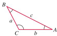
Exercises 71 and 72 are about the triangle shown here.
-
Express A implicitly as a function of
𝑎 , 𝑏 , 𝜕 𝐴 / 𝜕 𝑏 -
Express a implicitly as a function of A, b, and B and calculate ∂ ∂ a A and ∂ ∂ a B.
-
Two dependent variables Express
𝑣 𝑥 𝑥 = 𝑣 𝑦 = 𝑢 i f 𝑣 𝑥 𝑣 𝑥 𝑢 𝑥 . ) -
Two dependent variables Find
𝜕 𝑥 / 𝜕 𝑢 𝜕 𝑦 / 𝜕 𝑢 𝑢 = 𝑥 2 − 𝑦 2 𝑣 = 𝑥 2 − 𝑦 𝑣 , 𝑠 = 𝑥 2 + 𝑦 2 𝜕 𝑠 / 𝜕 𝑢
Theory and Examples
-
Let
𝑓 ( 𝑥 , 𝑦 ) = 2 𝑥 + 3 𝑦 − 4 𝑥 = 2 𝑦 = − 1 -
Let
𝑓 ( 𝑥 , 𝑦 ) = 𝑥 2 + 𝑦 3 . 𝑥 = − 1 𝑦 = 1 .
In Exercises 77–80, find a function
𝜕 𝑓 𝜕 𝑥 = 3 𝑥 2 𝑦 2 − 2 𝑥 , 𝜕 𝑓 𝜕 𝑦 = 2 𝑥 3 𝑦 + 6 𝑦
c o t f ( 𝑥 , 𝑦 ) = { 𝑦 3 , 𝑦 ≥ 0 − 𝑦 2 , 𝑦 < 0 .
Find
- Let
𝑓 ( 𝑥 , 𝑦 ) = ⎧ { { ⎨ { { ⎩ 𝑥 𝑦 𝑥 2 − 𝑦 2 𝑥 2 + 𝑦 2 , i f ( 𝑥 , 𝑦 ) ≠ 0 , 0 , i f ( 𝑥 , 𝑦 ) = 0 .
a. Show that
b. Show that
The three-dimensional Laplace equation
is satisfied by steady-state temperature distributions
obtained by dropping the
Show that each function in Exercises 83–90 satisfies a Laplace equation.
-
𝑓 ( 𝑥 , 𝑦 , 𝑧 ) = 𝑥 2 + 𝑦 2 − 2 𝑧 2 -
𝑓 ( 𝑥 , 𝑦 , 𝑧 ) = 2 𝑧 3 − 3 ( 𝑥 2 + 𝑦 2 ) 𝑧 -
𝑓 ( 𝑥 , 𝑦 ) = 𝑒 − 2 𝑦 c o s 2 𝑥 -
𝑓 ( 𝑥 , 𝑦 ) = l n √ 𝑥 2 + 𝑦 2 -
𝑓 ( 𝑥 , 𝑦 ) = 3 𝑥 + 2 𝑦 − 4 -
𝑓 ( 𝑥 , 𝑦 ) = a r c t a n 𝑥 𝑦
The wave equation If we stand on an ocean shore and take a snapshot of the waves, the picture shows a regular pattern of peaks and valleys in an instant of time. We see periodic vertical motion in space, with respect to distance. If we stand in the water, we can feel the rise and fall of the water as the waves go by. We see periodic vertical motion in time. In physics, this beautiful symmetry is expressed by the one-dimensional wave equation
where w is the wave height, x is the distance variable, t is the time variable, and c is the velocity with which the waves are propagated.
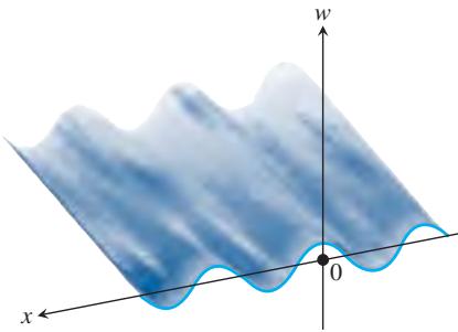
In our example, x is the distance across the ocean’s surface, but in other applications, x might be the distance along a vibrating string, distance through air (sound waves), or distance through space (light waves). The number c varies with the medium and type of wave.
Show that the functions in Exercises 91–97 are all solutions of the wave equation.
-
𝑤 = s i n ( 𝑥 + 𝑐 𝑡 ) -
𝑤 = c o s ( 2 𝑥 + 2 𝑐 𝑡 ) -
𝑤 = s i n ( 𝑥 + 𝑐 𝑡 ) + c o s ( 2 𝑥 + 2 𝑐 𝑡 ) -
w x ct= +ln 2 2( )
-
w x ct= −tan 2 2( )
-
𝑤 = 5 c o s ( 3 𝑥 + 3 𝑐 𝑡 ) + 𝑒 𝑥 + 𝑐 𝑡 -
𝑤 = 𝑓 ( 𝑢 ) , \ b o l d s y m b o l 𝑢 = \ b o l d s y m b o l 𝑎 ( \ b o l d s y m b o l 𝑥 + \ b o l d s y m b o l 𝑐 𝑡 ) -
Does a function
𝑓 ( 𝑥 , 𝑦 ) -
If a function
𝑓 ( 𝑥 , 𝑦 ) -
The heat equation An important partial differential equation that describes the distribution of heat in a region at time t can be represented by the one-dimensional heat equation
Show that
- Let
𝑓 ( 𝑥 , 𝑦 ) = ⎧ { { ⎨ { { ⎩ 𝑥 𝑦 2 𝑥 2 + 𝑦 4 , ( 𝑥 , 𝑦 ) ≠ ( 0 , 0 ) 0 , ( 𝑥 , 𝑦 ) = ( 0 , 0 ) .
Show that
- Let
𝑓 ( 𝑥 , 𝑦 ) = { 0 , 𝑥 2 < 𝑦 < 2 𝑥 2 1 , o t h e r w i s e .
Show that
- The Korteweg–de Vries equation
This nonlinear differential equation, which describes wave motion on shallow water surfaces, is given by
Show that
- Show that
𝑇 = 1 √ 𝑥 2 + 𝑦 2 𝑇 𝑥 𝑥 + 𝑇 𝑦 𝑦 = 𝑇 3 .
13.4 The Chain Rule
To find
The Chain Rule for functions of a single variable studied in Section 3.6 says that if
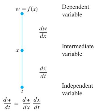
For this composite function
For functions of several variables the Chain Rule has more than one form, which depends on how many independent and intermediate variables are involved. However, once the variables are taken into account, the Chain Rule works in the same way we just discussed.
Functions of Two Variables
The Chain Rule formula for a differentiable function
THEOREM 5—Chain Rule for Functions of One Independent Variable and Two Intermediate Variables
If
or
Each of
To remember the Chain Rule, picture the diagram below. To find
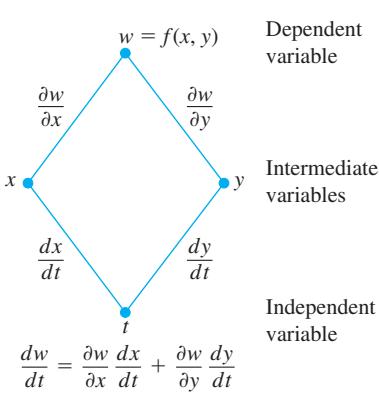
Proof The proof consists of showing that if x and y are differentiable at
where
Let
where
Letting
Often we write
However, the meaning of the dependent variable w is different on each side of the preceding equation. On the left-hand side, it refers to the composite function
The dependency diagram on the preceding page provides a convenient way to remember the Chain Rule. The “true” independent variable in the composite function is t, whereas x and
A more precise notation for the Chain Rule shows where the various derivatives in Theorem 5 are evaluated:
or, using another notation,
EXAMPLE 1 Use the Chain Rule to find the derivative of
with respect to t along the path
Solution We apply the Chain Rule to find dw dt as follows:
In this example, we can check the result with a more direct calculation. As a function of t,
so
In either case, at the given value of t,
Functions of Three Variables
You can probably predict the Chain Rule for functions of three intermediate variables, as it involves adding the expected third term to the two-variable formula.
Here we have three routes from w to t instead of two, but finding dw dt is still the same. Read down each route, multiplying derivatives along the way; then add.
Chain Rule
THEOREM 6—Chain Rule for Functions of One Independent Variable and Three Intermediate Variables
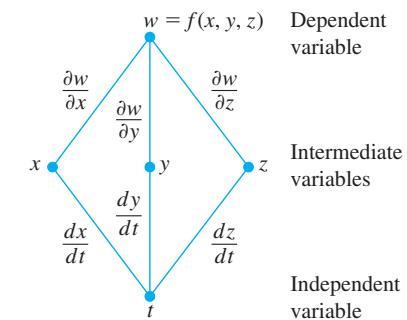
If
The proof is identical to the proof of Theorem 5, except that there are now three intermediate variables instead of two. The dependency diagram we use for remembering the new equation is similar as well, with three routes from w to t.
EXAMPLE 2 Find dw dt if
In this example the values of
Solution Using the Chain Rule for three intermediate variables, we have
SO
For a physical interpretation of change along a curve, think of an object whose position is changing with time t. If
Functions Defined on Surfaces
If we are interested in the temperature
Under the conditions stated below, w has partial derivatives with respect to both r and s that can be calculated in the following way.
THEOREM 7—Chain Rule for Two Independent Variables and Three Intermediate Variables
Suppose that
The first of these equations can be derived from the Chain Rule in Theorem 6 by holding s fixed and treating r as t. The second can be derived in the same way, holding r fixed and treating s as t. The dependency diagrams for both equations are shown in Figure 13.22.
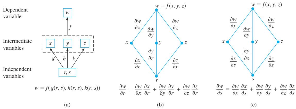
FIGURE 13.22 Composite function and dependency diagrams for Theorem 7.
EXAMPLE 3 Express
Solution Using the formulas in Theorem 7, we find
Chain Rule
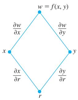
If
FIGURE 13.23 Dependency diagram for the equation
Figure 13.23 shows the dependency diagram for the first of these equations. The diagram for the second equation is similar; just replace r with s.
EXAMPLE 4 Express
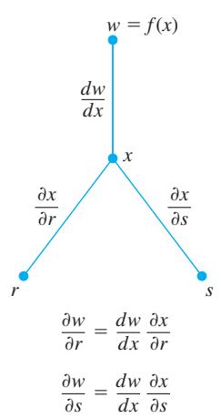
FIGURE 13.24 Dependency diagram for differentiating f as a composite function of r and s with one intermediate variable.
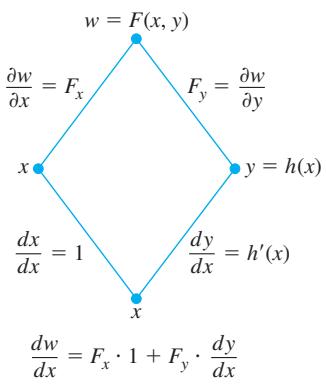
FIGURE 13.25 Dependency diagram for differentiating
Solution The preceding discussion gives the following.
If
In this case, we use the ordinary (single-variable) derivative, dw/dx. The dependency diagram is shown in Figure 13.24.
Implicit Differentiation Revisited
The two-variable Chain Rule in Theorem 5 leads to a formula that takes some of the algebra out of implicit differentiation. Suppose that
-
The function
𝐹 ( 𝑥 , 𝑦 ) -
The equation
𝐹 ( 𝑥 , ℎ ( 𝑥 ) ) = 0 𝑦 = ℎ ( 𝑥 )
Since
If
We state this result formally.
THEOREM 8—A Formula for Implicit Differentiation
Suppose that
EXAMPLE 5 Use Theorem 8 to find dy/dx if
Solution Take
This calculation is significantly shorter than a single-variable calculation using implicit differentiation.
The result in Theorem 8 is easily extended to three variables. Suppose that the equation
SO
A similar calculation for differentiating with respect to the independent variable y gives
Whenever
An important result from advanced calculus, called the Implicit Function Theorem, states the conditions for which our results in Equations (2) are valid. If the partial derivatives
Solution Let
Since
At
Functions of Many Variables
We have seen several different forms of the Chain Rule in this section, but each one is just a special case of one general formula. When solving particular problems, it may help to draw the appropriate dependency diagram by placing the dependent variable on top, the intermediate variables in the middle, and the selected independent variable at the bottom. To find the derivative of the dependent variable with respect to the selected independent variable, start at the dependent variable and read down each route of the dependency diagram to the independent variable, calculating and multiplying the derivatives along each route. Then add the products found for the different routes.
In general, suppose that
One way to remember this equation is to think of the right-hand side as the dot product of two n-dimensional vectors:
The first vector describes how w changes in various directions, while the second vector indicates the velocity vector of
EXERCISES 13.4
Chain Rule: One Independent Variable
In Exercises 1–6, (a) express dw/dt as a function of t, both by using the Chain Rule and by expressing w in terms of t and differentiating directly with respect to t. Then (b) evaluate dw/dt at the given value of t.
𝑤 = 𝑧 − s i n 𝑥 𝑦 , 𝑥 = 𝑡 , 𝑦 = l n 𝑡 , 𝑧 = 𝑒 𝑡 − 1 ; 𝑡 = 1
Chain Rule: Two and Three Independent Variables
In Exercises 7 and 8, (a) express
In Exercises 9 and 10, (a) express
𝑤 = l n ( 𝑥 2 + 𝑦 2 + 𝑧 2 ) , 𝑥 = 𝑢 𝑒 𝑣 s i n 𝑢 , 𝑦 = 𝑢 𝑒 𝑣 c o s 𝑢 , 𝑧 = 𝑢 𝑒 𝑣 ; ( 𝑢 , 𝑣 ) = ( − 2 , 0 )
In Exercises 11 and 12, (a) express
𝑢 = 𝑝 − 𝑞 𝑞 − 𝑟 , 𝑝 = 𝑥 + 𝑦 + 𝑧 , 𝑞 = 𝑥 − 𝑦 + 𝑧 ,
𝑢 = 𝑒 𝑞 𝑟 s i n − 1 𝑝 , 𝑝 = s i n 𝑥 , 𝑞 = 𝑧 2 l n 𝑦 , 𝑟 = 1 / 𝑧 ; ( 𝑥 , 𝑦 , 𝑧 ) = ( 𝜋 / 4 , 1 / 2 , − 1 / 2 )
Using a Dependency Diagram
In Exercises 13–24, draw a dependency diagram and write a Chain Rule formula for each derivative.
𝑑 𝑧 𝑑 𝑡 𝑧 = 𝑓 ( 𝑥 , 𝑦 ) 𝑥 = 𝑔 ( 𝑡 ) 𝑦 = ℎ ( 𝑡 )
-
𝜕 𝑤 𝜕 𝑢 𝜕 𝑤 𝜕 𝑣 𝑤 = 𝑔 ( 𝑥 , 𝑦 ) 𝑥 = ℎ ( 𝑢 , 𝑣 ) 𝑦 = 𝑘 ( 𝑢 , 𝑣 ) -
𝜕 𝑤 𝜕 𝑥 𝜕 𝑤 𝜕 𝑦 𝑤 = 𝑔 ( 𝑢 , 𝑣 ) 𝑢 = ℎ ( 𝑥 , 𝑦 ) 𝑣 = 𝑘 ( 𝑥 , 𝑦 ) -
𝜕 𝑧 𝜕 𝑡 a n d 𝜕 𝑧 𝜕 𝑠 f o r 𝑧 = 𝑓 ( 𝑥 , 𝑦 ) , 𝑥 = 𝑔 ( 𝑡 , 𝑠 ) , 𝑦 = ℎ ( 𝑡 , 𝑠 ) -
𝜕 𝑦 𝜕 𝑟 𝑦 = 𝑓 ( 𝑢 ) , 𝑢 = 𝑔 ( 𝑟 , 𝑠 ) -
𝜕 𝑤 𝜕 𝑠 𝜕 𝑤 𝜕 𝑡 𝑤 = 𝑔 ( 𝑢 ) 𝑢 = ℎ ( 𝑠 , 𝑡 ) -
𝜕 𝑤 𝜕 𝑝 𝑤 = 𝑓 ( 𝑥 , 𝑦 , 𝑧 , 𝑣 ) 𝑥 = 𝑔 ( 𝑝 , 𝑞 ) 𝑦 = ℎ ( 𝑝 , 𝑞 ) 𝑧 = 𝑗 ( 𝑝 , 𝑞 ) 𝑣 = 𝑘 ( 𝑝 , 𝑞 ) -
𝜕 𝑤 𝜕 𝑟 𝜕 𝑤 𝜕 𝑠 𝑤 = 𝑓 ( 𝑥 , 𝑦 ) 𝑥 = 𝑔 ( 𝑟 ) 𝑦 = ℎ ( 𝑠 ) -
𝜕 𝑤 𝜕 𝑠 𝑤 = 𝑔 ( 𝑥 , 𝑦 ) 𝑥 = ℎ ( 𝑟 , 𝑠 , 𝑡 ) 𝑦 = 𝑘 ( 𝑟 , 𝑠 , 𝑡 )
Implicit Differentiation
Assuming that the equations in Exercises 25–30 define y as a differentiable function of x, use Theorem 8 to find the value of dy/dx at the given point.
-
𝑥 3 − 2 𝑦 2 + 𝑥 𝑦 = 0 , ( 1 , 1 ) -
𝑥 𝑦 + 𝑦 2 − 3 𝑥 − 3 = 0 , ( − 1 , 1 ) -
𝑥 2 + 𝑥 𝑦 + 𝑦 2 − 7 = 0 -
𝑥 𝑒 𝑦 + s i n 𝑥 𝑦 + 𝑦 − l n 2 = 0 , ( 0 , l n 2 ) -
( 𝑥 3 − 𝑦 4 ) 6 + l n ( 𝑥 2 + 𝑦 ) = 1 , ( − 1 , 0 ) -
𝑥 𝑒 𝑥 2 𝑦 − 𝑦 𝑒 𝑥 = 𝑥 + 𝑦 − 2 ,
Find the values of
-
𝑧 3 − 𝑥 𝑦 + 𝑦 𝑧 + 𝑦 3 − 2 = 0 , ( 1 , 1 , 1 ) -
1 𝑥 + 1 𝑦 + 1 𝑧 − 1 = 0 , -
s i n ( 𝑥 + 𝑦 ) + s i n ( 𝑦 + 𝑧 ) + s i n ( 𝑥 + 𝑧 ) = 0 , ( 𝜋 , 𝜋 , 𝜋 ) -
𝑥 𝑒 𝑦 + 𝑦 𝑒 𝑧 + 2 l n 𝑥 − 2 − 3 l n 2 = 0 , ( 1 , l n 2 , l n 3 )
Finding Partial Derivatives at Specified Points
-
Find
𝜕 𝑤 / 𝜕 𝑟 𝑟 = 1 , 𝑠 = − 1 𝑤 = ( 𝑥 + 𝑦 + 𝑧 ) 2 𝑥 = 𝑟 − 𝑠 , 𝑦 = c o s ( 𝑟 + 𝑠 ) , 𝑧 = s i n ( 𝑟 + 𝑠 ) -
Find
𝜕 𝑤 / 𝜕 𝑣 𝑢 = − 1 , 𝑣 = 2 𝑤 = 𝑥 𝑦 + l n 𝑧 𝑥 = 𝑣 2 / 𝑢 , 𝑦 = 𝑢 + 𝑣 , 𝑧 = c o s 𝑢 -
Find
𝜕 𝑤 / 𝜕 𝑣 𝑢 = 0 , 𝑣 = 0 𝑤 = 𝑥 2 + ( 𝑦 / 𝑥 ) 𝑥 = 𝑢 − 2 𝑣 + 1 𝑦 = 2 𝑢 + 𝑣 − 2 -
Find
𝜕 𝑧 / 𝜕 𝑢 𝑢 = 0 , 𝑣 = 1 𝑧 = s i n 𝑥 𝑦 + 𝑥 s i n 𝑦 𝑥 = 𝑢 2 + 𝑣 2 𝑦 = 𝑢 𝑣 -
Find
𝜕 𝑧 / 𝜕 𝑢 𝜕 𝑧 / 𝜕 𝑣 𝑢 = l n 2 , 𝑣 = 1 𝑧 = 5 t a n − 1 𝑥 𝑥 = 𝑒 𝑢 + l n 𝑣 -
Find
𝜕 𝑧 / 𝜕 𝑢 𝜕 𝑧 / 𝜕 𝑣 𝑧 = l n 𝑞 𝑞 = √ 𝑣 + 3 t a n − 1 𝑢
Theory and Examples
-
Assume that
𝑤 = 𝑓 ( 𝑠 3 + 𝑡 2 ) 𝑓 ′ ( 𝑥 ) = 𝑒 𝑥 𝜕 𝑤 𝜕 𝑡 𝜕 𝑤 𝜕 𝑠 -
Assume that
𝑤 = 𝑓 ( 𝑡 𝑠 2 , 𝑠 𝑡 ) 𝜕 𝑓 𝜕 𝑥 ( 𝑥 , 𝑦 ) = 𝑥 𝑦 𝜕 𝑓 𝜕 𝑦 ( 𝑥 , 𝑦 ) = 𝑥 2 2 𝜕 𝑤 𝜕 𝑡 𝜕 𝑤 𝜕 𝑠 -
Assume that
𝑧 = 𝑓 ( 𝑥 , 𝑦 ) 𝑥 = 𝑔 ( 𝑡 ) 𝑦 = ℎ ( 𝑡 ) 𝑓 𝑥 ( 2 , − 1 ) = 3 𝑓 𝑦 ( 2 , − 1 ) = − 2 𝑔 ( 0 ) = 2 ℎ ( 0 ) = − 1 𝑔 ′ ( 0 ) = 5 ℎ ′ ( 0 ) = − 4 𝑑 𝑧 𝑑 𝑡 ∣ 𝑡 = 0 -
Assume that
𝑧 = 𝑓 ( 𝑥 , 𝑦 ) 2 𝑥 = 𝑔 ( 𝑡 ) 𝑦 = ℎ ( 𝑡 ) 𝑓 𝑥 ( 1 , 0 ) = − 1 𝑓 𝑦 ( 1 , 0 ) = 1 𝑓 ( 1 , 0 ) = 2 𝑔 ( 3 ) = 1 ℎ ( 3 ) = 0 𝑔 ′ ( 3 ) = − 3 ℎ ′ ( 3 ) = 4 𝑑 𝑧 𝑑 𝑡 ∣ 𝑡 = 3 -
Assume that
𝑧 = 𝑓 ( 𝑤 ) , 𝑤 = 𝑔 ( 𝑥 , 𝑦 ) , 𝑥 = 2 𝑟 3 − 𝑠 2 𝑦 = 𝑟 𝑒 𝑠 𝑔 𝑥 ( 2 , 1 ) = − 3 𝑔 𝑦 ( 2 , 1 ) = 2 𝑓 ′ ( 7 ) = − 1 𝑔 ( 2 , 1 ) = 7 𝜕 𝑧 𝜕 𝑟 ∣ 𝑟 = 1 , 𝑠 = 0 𝜕 𝑧 𝜕 𝑠 ∣ 𝑟 = 1 , 𝑠 = 0 -
Assume that
𝑧 = l n ( 𝑓 ( 𝑤 ) ) 𝑤 = 𝑔 ( 𝑥 , 𝑦 ) 𝑥 = √ 𝑟 − 𝑠 𝑦 = 𝑟 2 𝑠 𝑔 𝑥 ( 2 , − 9 ) = − 1 𝑔 𝑦 ( 2 , − 9 ) = 3 𝑓 ′ ( − 2 ) = 2 𝑓 ( − 2 ) = 5 𝑔 ( 2 , − 9 ) = − 2 𝜕 𝑧 𝜕 𝑟 ∣ 𝑟 = 3 , 𝑠 = − 1 𝜕 𝑧 𝜕 𝑠 ∣ 𝑟 = 3 , 𝑠 = − 1 -
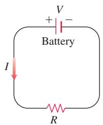
Changing voltage in a circuit The voltage V in a circuit that satisfies the law V = IR is slowly dropping as the battery wears out. At the same time, the resistance R is increasing as the resistor heats up. Use the equation
to find how the current is changing at the instant when R = 600 ohms, I = 0.04 amp, dR/dt = 0.5 ohm/s, and dV/dt = -0.01 volt/s.
-
Changing dimensions in a box The lengths
𝑎 𝑏 𝑐 𝑎 = 1 m 𝑏 = 2 m 𝑐 = 3 m 𝑑 𝑎 / 𝑑 𝑡 = 𝑑 𝑏 / 𝑑 𝑡 = 1 m / s 𝑑 𝑐 / 𝑑 𝑡 = − 3 m / s 𝑉 𝑆 -
If
𝑓 ( 𝑢 , 𝑣 , 𝑤 ) 𝑢 = 𝑥 − 𝑦 , 𝑣 = 𝑦 − 𝑧 𝑤 = 𝑧 − 𝑥
- Polar coordinates Suppose that we substitute polar coordinates
𝑥 = 𝑟 c o s 𝜃 𝑦 = 𝑟 s i n 𝜃 𝑤 = 𝑓 ( 𝑥 , 𝑦 )
a. Show that
and
b. Solve the equations in part (a) to express
c. Show that
-
Laplace equations Show that if
𝑤 = 𝑓 ( 𝑢 , 𝑣 ) 𝑓 𝑢 𝑢 + 𝑓 𝑣 𝑣 = 0 𝑢 = ( 𝑥 2 − 𝑦 2 ) / 2 𝑣 = 𝑥 𝑦 𝑤 𝑤 𝑥 𝑥 + 𝑤 𝑦 𝑦 = 0 -
Laplace equations Let
𝑤 = 𝑓 ( 𝑢 ) + 𝑔 ( 𝑣 ) 𝑢 = 𝑥 + 𝑖 𝑦 𝑖 = √ − 1 𝑤 𝑥 𝑥 + 𝑤 𝑦 𝑦 = 0 -
Extreme values on a helix Suppose that the partial derivatives of a function
𝑓 ( 𝑥 , 𝑦 , 𝑧 ) 𝑥 = c o s 𝑡 𝑦 = s i n 𝑡
At what points on the curve, if any, can
- Temperature on a circle Let
𝑇 = 𝑓 ( 𝑥 , 𝑦 ) ( 𝑥 , 𝑦 ) 𝑥 = c o s 𝑡 𝑦 = s i n 𝑡 0 ≤ 𝑡 ≤ 2 𝜋
a. Find where the maximum and minimum temperatures on the circle occur by examining the derivatives
b. Suppose that
- Temperature on an ellipse Let
𝑇 = 𝑔 ( 𝑥 , 𝑦 ) ( 𝑥 , 𝑦 )
and suppose that
a. Locate the maximum and minimum temperatures on the ellipse by examining dT/dt and
b. Suppose that
-
The temperature
𝑇 = 𝑇 ( 𝑥 , 𝑦 ) ( 𝑥 , 𝑦 ) 𝑇 𝑥 ( 1 , 2 ) = 3 𝑇 𝑦 ( 1 , 2 ) = − 1 𝑥 = 𝑒 2 𝑡 − 2 𝑦 = 2 + l n 𝑡 -
A bug crawls on the surface
𝑧 = 𝑥 2 − 𝑦 2 𝑥 = 𝑓 ( 𝑡 ) 𝑦 = 𝑔 ( 𝑡 ) 𝑓 ( 2 ) = 4 𝑓 ′ ( 2 ) = − 1 𝑔 ( 2 ) = − 2 𝑔 ′ ( 2 ) = − 3 𝑧 𝑡 = 2
Differentiating Integrals Under mild continuity restrictions, it is true that if
then
by letting
where
-
𝐹 ( 𝑥 ) = ∫ 𝑥 2 0 √ 𝑡 4 + 𝑥 3 𝑑 𝑡 -
𝐹 ( 𝑥 ) = ∫ 1 𝑥 2 √ 𝑡 3 + 𝑥 2 𝑑 𝑡 -
Water is flowing into a tank in the form of a right-circular cylinder at the rate of
( 4 / 5 ) 𝜋 𝑚 3 / 𝑚 𝑖 𝑛 2 0 𝜋 𝑚 3 -
Suppose
𝑓 𝑥 , 𝑦 𝑧 𝑢 = 𝑓 ( 𝑥 , 𝑦 , 𝑧 ) 𝑥 = 𝑟 s i n 𝜙 c o s 𝜃 , 𝑦 = 𝑟 s i n 𝜙 s i n 𝜃 𝑧 = 𝑟 c o s 𝜙 𝜕 𝑢 / 𝜕 𝑟 𝜕 𝑢 / 𝜕 𝜙 𝜕 𝑢 / 𝜕 𝜃 𝜕 𝑢 / 𝜕 𝑥 , 𝜕 𝑢 / 𝜕 𝑦 𝜕 𝑢 / 𝜕 𝑧 -
At a given instant, the length of one leg of a right triangle is 10 m, and it is increasing at the rate of 1 m/min, and the length of the other leg of the right triangle is 12 m, and it is decreasing at the rate of 2 m/min. Find the rate of change of the measure of the acute angle opposite the leg of length 12 m at the given instant.
13.5 Directional Derivatives and Gradient Vectors
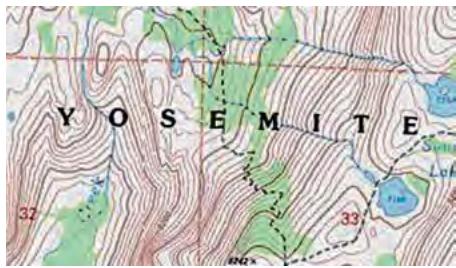
FIGURE 13.26 Contours within Yosemite National Park in California show streams, which follow paths of steepest descent, running perpendicular to the contours. (Source: Yosemite National Park Map from U.S. Geological Survey, http://www.usgs.gov)
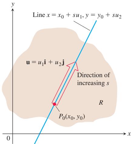
FIGURE 13.27 The rate of change of f in the direction of u at a point
If you look at the map (Figure 13.26) showing contours within Yosemite National Park in California, you will notice that the streams flow perpendicular to the contours. The streams are following paths of steepest descent so the waters reach lower elevations as quickly as possible. Therefore, the fastest instantaneous rate of change in a stream’s elevation above sea level has a particular direction. In this section, you will see why this direction, called the “downhill” direction, is perpendicular to the contours.
Directional Derivatives in the Plane
We know from Section 13.4 that if
At any point
Suppose that the function
parametrize the line through
DEFINITION The derivative of
at 𝑓 in the direction of the unit vector 𝑃 0 ( 𝑥 0 , 𝑦 0 ) is the number 𝐮 = 𝑢 1 𝐢 + 𝑢 2 𝐣 ( 𝑑 𝑓 𝑑 𝑠 ) 𝐮 , 𝑃 0 = l i m 𝑠 → 0 𝑓 ( 𝑥 0 + 𝑠 𝑢 1 , 𝑦 0 + 𝑠 𝑢 2 ) − 𝑓 ( 𝑥 0 , 𝑦 0 ) 𝑠 , ( 1 ) provided the limit exists.
The directional derivative defined by Equation (1) is also denoted by
The partial derivatives
EXAMPLE 1 Using the definition, find the derivative of
at
Solution Applying the definition in Equation (1), we obtain
The rate of change of
Interpretation of the Directional Derivative
The equation
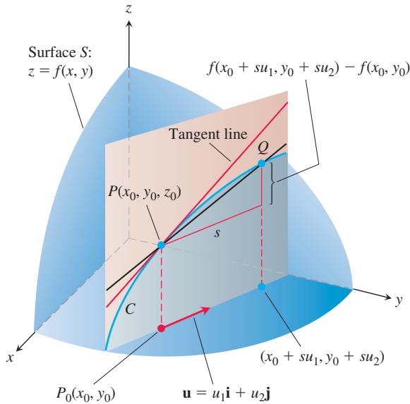
FIGURE 13.28 The slope of the trace curve
When
For a physical interpretation of the directional derivative, suppose that
Calculation and Gradients
We now develop an efficient formula to calculate the directional derivative for a differentiable function f. We begin with the line
through
Equation (3) says that the derivative of a differentiable function
DEFINITION The gradient vector (or gradient) of
is the vector 𝑓 ( 𝑥 , 𝑦 ) ∇ 𝑓 = 𝜕 𝑓 𝜕 𝑥 𝐢 + 𝜕 𝑓 𝜕 𝑦 𝐣 .
The value of the gradient vector obtained by evaluating the partial derivatives at a point
The notation
THEOREM 9—The Directional Derivative Is a Dot Product
If
the dot product of the gradient
EXAMPLE 2 Find the derivative of
Solution Recall that the direction of a vector v is the unit vector obtained by dividing v by its length:
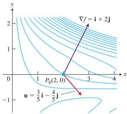
FIGURE 13.29 Picture
The partial derivatives of f are everywhere continuous and at
The gradient of
(Figure 13.29). The derivative of
Eq. (4) with the
Evaluating the dot product in the brief version of Equation (4) gives
where
Properties of the Directional Derivative 𝐷 𝑢 𝑓 = ∇ 𝑓 ⋅ 𝑢 = | ∇ 𝑓 | c o s 𝜃
- The function f increases most rapidly when
c o s 𝜃 = 1 𝜃 = 0 ∇ 𝑓 ∇ 𝑓
-
Similarly, f decreases most rapidly in the direction of
− ∇ 𝑓 𝐷 𝐮 𝑓 = | ∇ 𝑓 | c o s ( 𝜋 ) = − | ∇ 𝑓 | -
Any direction
𝐮 ∇ 𝑓 ≠ 0 𝑓 𝜃 𝜋 / 2
As we discuss later, these properties hold in three dimensions as well as two.
EXAMPLE 3 Find the directions in which
(a) increases most rapidly at the point
(b) decreases most rapidly at
(c) What are the directions of zero change in
Solution
(a) The function increases most rapidly in the direction of
Its direction is
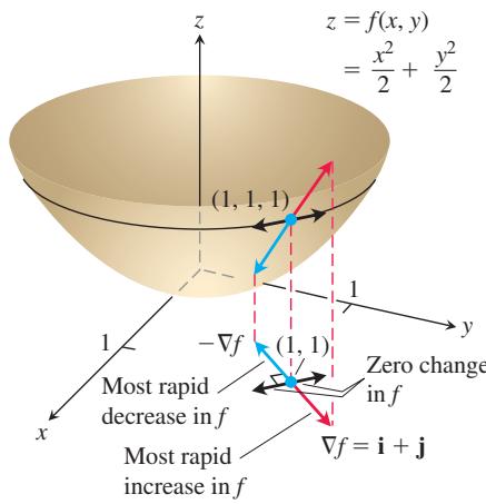
FIGURE 13.30 The direction in which
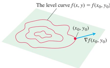
FIGURE 13.31 When it is nonzero, the gradient of a differentiable function of two variables at a point is always normal to the function’s level curve through that point.
(b) The function decreases most rapidly in the direction of
(c) The directions of zero change at
See Figure 13.30.
Gradients and Tangents to Level Curves
If a differentiable function
Assuming the gradient of f is a nonzero vector, Equation (5) says that
At every point
Equation (5) validates our observation that streams flow perpendicular to the contours in topographical maps (see Figure 13.26). Since the downflowing stream will reach its destination in the fastest way, it must flow in the direction of the negative gradient vectors from Property 2 for the directional derivative. Equation (5) tells us these directions are perpendicular to the level curves.
This observation also enables us to find equations for tangent lines to level curves. They are the lines normal to the gradients. The line through a point
(Exercise 39). If
Equation for the Tangent Line to a Level Curve
EXAMPLE 4 Find an equation for the tangent to the ellipse
(Figure 13.32) at the point
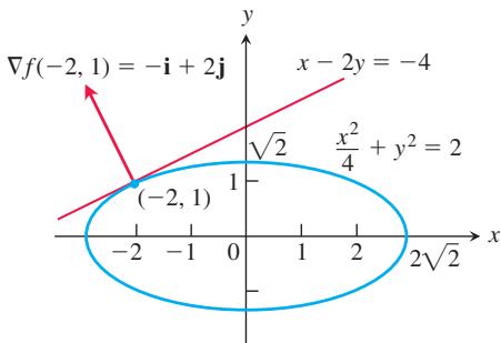
Solution The ellipse is a level curve of the function
FIGURE 13.32 We can find the tangent to the ellipse
The gradient of
Because this gradient vector is nonzero, the tangent to the ellipse at
If we know the gradients of two functions f and g, we automatically know the gradients of their sum, difference, constant multiples, product, and quotient. You are asked to establish the following rules in Exercise 40. Notice that these rules have the same form as the corresponding rules for derivatives of single-variable functions.
Algebra Rules for Gradients
- Sum Rule:
- Difference Rule:
- Constant Multiple Rule:
- Product Rule:
- Quotient Rule:
Scalar multipliers on left of gradients
EXAMPLE 5 We illustrate two of the rules with
We have
∇ ( 𝑓 − 𝑔 ) = ∇ ( 𝑥 − 4 𝑦 ) = 𝐢 − 4 𝐣 = ∇ 𝑓 − ∇ 𝑔
Rule 2
∇ ( 𝑓 𝑔 ) = ∇ ( 3 𝑥 𝑦 − 3 𝑦 2 ) = 3 𝑦 𝑖 + ( 3 𝑥 − 6 𝑦 ) 𝑗
and
Substitute.
Simplify.
We have therefore verified that for this example,
Functions of Three Variables
For a differentiable function
and
The directional derivative can once again be written in the form
so the properties listed earlier for functions of two variables extend to three variables. At any given point, f increases most rapidly in the direction of
EXAMPLE 6
(a) Find the derivative of
(b) In what directions does
Solution
(a) The direction of v is obtained by dividing v by its length:
The partial derivatives of f at
The gradient of
The derivative of
(b) The function increases most rapidly in the direction of
Functions of More Than Three Variables
The gradient of a differentiable function of n variables
If
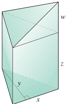
FIGURE 13.33 A tetrahedron on top of a triangular prism (Example 7).
EXAMPLE 7 The volume of the solid shown in Figure 13.33 consisting of a tetrahedron on top of a triangular prism is given by
(a) Calculate the derivative of
(b) What is the geometric significance of the value obtained in part (a)?
Solution
(a) The direction of v is the unit vector
The four partial derivatives of
The gradient of
The derivative of f at
(b) Geometrically, this means that if the dimensions are
The Chain Rule for Paths
If
The partial derivatives on the right-hand side of the above equation are evaluated along the curve
The Derivative Along a Path
What Equation (7) says is that the derivative of the composite function
EXERCISES 13.5
Calculating Gradients
In Exercises 1–6, find the gradient of the function at the given point. Then sketch the gradient, together with the level curve that passes through the point.
-
𝑓 ( 𝑥 , 𝑦 ) = 𝑦 − 𝑥 , ( 2 , 1 ) -
𝑓 ( 𝑥 , 𝑦 ) = l n ( 𝑥 2 + 𝑦 2 )
(1,1)
-
𝑔 ( 𝑥 , 𝑦 ) = 𝑥 𝑦 2 ( 2 , − 1 ) -
𝑔 ( 𝑥 , 𝑦 ) = 𝑥 2 2 − 𝑦 2 2 , ( √ 2 , 1 ) -
𝑓 ( 𝑥 , 𝑦 ) = √ 2 𝑥 + 3 𝑦 , ( − 1 , 2 ) -
𝑓 ( 𝑥 , 𝑦 ) = t a n − 1 √ 𝑥 𝑦 , ( 4 , − 2 )
In Exercises 7–10, find
-
𝑓 ( 𝑥 , 𝑦 , 𝑧 ) = 𝑥 2 + 𝑦 2 − 2 𝑧 2 + 𝑧 l n 𝑥 , ( 1 , 1 , 1 ) -
𝑓 ( 𝑥 , 𝑦 , 𝑧 ) = 2 𝑧 3 − 3 ( 𝑥 2 + 𝑦 2 ) 𝑧 + a r c t a n 𝑥 𝑧 , ( 1 , 1 , 1 ) -
𝑓 ( 𝑥 , 𝑦 , 𝑧 ) = ( 𝑥 2 + 𝑦 2 + 𝑧 2 ) − 1 / 2 + l n ( 𝑥 𝑦 𝑧 ) , ( − 1 , 2 , − 2 ) -
𝑓 ( 𝑥 , 𝑦 , 𝑧 ) = 𝑒 𝑥 + 𝑦 c o s 𝑧 + ( 𝑦 + 1 ) a r c s i n 𝑥 , ( 0 , 0 , 𝜋 / 6 )
Finding Directional Derivatives
In Exercises 11–18, find the derivative of the function at
-
𝑓 ( 𝑥 , 𝑦 ) = 2 𝑥 𝑦 − 3 𝑦 2 , 𝑃 0 ( 5 , 5 ) , 𝐯 = 4 𝐢 + 3 𝐣 -
𝑓 ( 𝑥 , 𝑦 ) = 2 𝑥 2 + 𝑦 2 , 𝑃 0 ( − 1 , 1 ) , 𝐯 = 3 𝐢 − 4 𝐣 -
𝑔 ( 𝑥 , 𝑦 ) = 𝑥 − 𝑦 𝑥 𝑦 + 2 , 𝑃 0 ( 1 , − 1 ) , 𝐯 = 1 2 𝐢 + 5 𝐣 -
ℎ ( 𝑥 , 𝑦 ) = a r c t a n ( 𝑦 / 𝑥 ) + √ 3 a r c s i n ( 𝑥 𝑦 / 2 ) , 𝑃 0 ( 1 , 1 ) , 𝐯 = 3 𝐢 − 2 𝐣 -
𝑓 ( 𝑥 , 𝑦 , 𝑧 ) = 𝑥 𝑦 + 𝑦 𝑧 + 𝑧 𝑥 , 𝑃 0 ( 1 , − 1 , 2 ) , 𝐯 = 3 𝐢 + 6 𝐣 − 2 𝐤 -
𝑓 ( 𝑥 , 𝑦 , 𝑧 ) = 𝑥 2 + 2 𝑦 2 − 3 𝑧 2 , 𝑃 0 ( 1 , 1 , 1 ) , 𝐯 = 𝐢 + 𝐣 + 𝐤 -
𝑔 ( 𝑥 , 𝑦 , 𝑧 ) = 3 𝑒 𝑥 c o s 𝑦 𝑧 , 𝑃 0 ( 0 , 0 , 0 ) , 𝐯 = 2 𝐢 + 𝐣 − 2 𝐤 -
ℎ ( 𝑥 , 𝑦 , 𝑧 ) = c o s 𝑥 𝑦 + 𝑒 𝑦 𝑧 + l n 𝑧 𝑥 , 𝑃 0 ( 1 , 0 , 1 / 2 ) ,
In Exercises 19–24, find the directions in which the functions increase most rapidly, and the directions in which they decrease most rapidly, at
-
𝑓 ( 𝑥 , 𝑦 ) = 𝑥 2 + 𝑥 𝑦 + 𝑦 2 , 𝑃 0 ( − 1 , 1 ) -
𝑓 ( 𝑥 , 𝑦 ) = 𝑥 2 𝑦 + 𝑒 𝑥 𝑦 s i n 𝑦 , 𝑃 0 ( 1 , 0 ) -
𝑓 ( 𝑥 , 𝑦 , 𝑧 ) = ( 𝑥 / 𝑦 ) − 𝑦 𝑧 , 𝑃 0 ( 4 , 1 , 1 ) -
𝑔 ( 𝑥 , 𝑦 , 𝑧 ) = 𝑥 𝑒 𝑦 + 𝑧 2 , 𝑃 0 ( 1 , l n 2 , 1 / 2 ) -
𝑓 ( 𝑥 , 𝑦 , 𝑧 ) = l n 𝑥 𝑦 + l n 𝑦 𝑧 + l n 𝑥 𝑧 , 𝑃 0 ( 1 , 1 , 1 ) -
ℎ ( 𝑥 , 𝑦 , 𝑧 ) = l n ( 𝑥 2 + 𝑦 2 − 1 ) + 𝑦 + 6 𝑧 , 𝑃 0 ( 1 , 1 , 0 )
Tangent Lines to Level Curves
In Exercises 25–28, sketch the curve
-
𝑥 2 + 𝑦 2 = 4 ( √ 2 , √ 2 ) -
𝑥 2 − 𝑦 = 1 ( √ 2 , 1 ) -
𝑥 𝑦 = − 4 , ( 2 , − 2 ) -
𝑥 2 − 𝑥 𝑦 + 𝑦 2 = 7 , ( − 1 , 2 )
Theory and Examples
-
Let
𝑓 ( 𝑥 , 𝑦 ) = 𝑥 2 − 𝑥 𝑦 + 𝑦 2 − 𝑦 𝐮 𝐷 𝐮 𝑓 ( 1 , − 1 )
a.𝐷 𝐮 𝑓 ( 1 , − 1 ) 𝐷 𝐮 𝑓 ( 1 , − 1 )
c.𝐷 𝐮 𝑓 ( 1 , − 1 ) = 0 𝐷 𝐮 𝑓 ( 1 , − 1 ) = 4 𝐷 𝐮 𝑓 ( 1 , − 1 ) = − 3 -
Let
𝑓 ( 𝑥 , 𝑦 ) = ( 𝑥 − 𝑦 ) ( 𝑥 + 𝑦 ) 𝐮 𝐷 𝐮 𝑓 ( − 1 2 , 3 2 )
a.𝐷 𝐮 𝑓 ( − 1 2 , 3 2 )
b.𝐷 𝐮 𝑓 ( − 1 2 , 3 2 )
c.𝐷 𝐮 𝑓 ( − 1 2 , 3 2 ) = 0 𝐷 𝐮 𝑓 ( − 1 2 , 3 2 ) = − 2 𝐷 𝐮 𝑓 ( − 1 2 , 3 2 ) = 1 -
Zero directional derivative In what direction is the derivative of
𝑓 ( 𝑥 , 𝑦 ) = 𝑥 𝑦 + 𝑦 2 𝑃 ( 3 , 2 ) -
Zero directional derivative In what directions is the derivative of
𝑓 ( 𝑥 , 𝑦 ) = ( 𝑥 2 − 𝑦 2 ) / ( 𝑥 2 + 𝑦 2 ) 𝑃 ( 1 , 1 ) -
Is there a direction
𝐮 𝑓 ( 𝑥 , 𝑦 ) = 𝑥 2 − 3 𝑥 𝑦 + 4 𝑦 2 𝑃 ( 1 , 2 ) -
Changing temperature along a circle Is there a direction u in which the rate of change of the temperature function
𝑇 ( 𝑥 , 𝑦 , 𝑧 ) = 2 𝑥 𝑦 − 𝑦 𝑧 𝑃 ( 1 , − 1 , 1 ) − 3 ∘ 𝐶 / 𝑚 -
The derivative of
𝑓 ( 𝑥 , 𝑦 ) 𝑃 0 ( 1 , 2 ) 𝐢 + 𝐣 2 √ 2 − 2 𝐣 − 3 𝑓 − 𝐢 − 2 𝐣 -
The derivative of
𝑓 ( 𝑥 , 𝑦 , 𝑧 ) 𝑣 = 𝑖 + 𝑗 − 𝑘 2 √ 3
a. What is
b. What is the derivative of
-
Directional derivatives and scalar components How is the derivative of a differentiable function
𝑓 ( 𝑥 , 𝑦 , 𝑧 ) 𝑃 0 𝐮 ∇ 𝑓 | 𝑃 0 𝐮 -
Directional derivatives and partial derivatives Assuming that the necessary derivatives of
𝑓 ( 𝑥 , 𝑦 , 𝑧 ) 𝐷 𝑖 𝑓 , 𝐷 𝑗 𝑓 𝐷 𝑘 𝑓 𝑓 𝑥 , 𝑓 𝑦 𝑓 𝑧 -
Lines in the xy-plane Show that
𝐴 ( 𝑥 − 𝑥 0 ) + 𝐵 ( 𝑦 − 𝑦 0 ) = 0 ( 𝑥 0 , 𝑦 0 ) 𝑁 = 𝐴 𝑖 + 𝐵 𝑗 -
The algebra rules for gradients Given a constant
𝑘
establish the algebra rules for gradients.
In Exercises 41–44, find a parametric equation for the line that is perpendicular to the graph of the given equation at the given point.
-
𝑥 2 + 𝑦 2 = 2 5 , ( − 3 , 4 ) -
𝑥 2 + 𝑥 𝑦 + 𝑦 2 = 3 , ( 2 , − 1 ) -
𝑥 2 + 𝑦 2 + 𝑧 2 = 1 4 , ( 3 , − 2 , 1 ) -
𝑧 = 𝑥 3 − 𝑥 𝑦 2 , ( − 1 , 1 , 0 )
Gradients and Directional Derivatives for Functions of More Than Three Variables
In Exercises 45–48, find
In Exercises 49–52, find the derivative of the function at
𝑓 ( 𝑥 , 𝑦 , 𝑧 , 𝑤 ) = 𝑤 l n 𝑥 𝑦 2 𝑧 3 , 𝑃 0 ( 𝑒 2 , − 2 , 1 , − 3 ) , 𝐯 = ⟨ − 1 , 2 , − 2 , 4 ⟩
13.6 Tangent Planes and Differentials
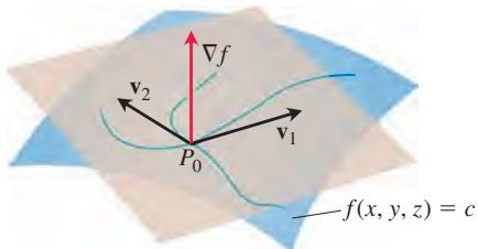
FIGURE 13.34 The gradient
In single-variable differential calculus, we saw how the derivative defined the tangent line to the graph of a differentiable function at a point on the graph. The tangent line then provided for a linearization of the function at the point. In this section, we will see analogously how the gradient defines the tangent plane to the level surface of a function
Tangent Planes and Normal Lines
If
Since
Now let us restrict our attention to the curves that pass through a point
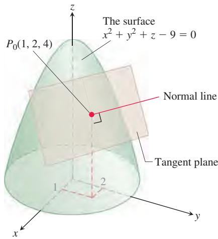
FIGURE 13.35 The tangent plane and normal line to this level surface at
DEFINITIONS The tangent plane to the level surface
of a differentiable function f at a point 𝑓 ( 𝑥 , 𝑦 , 𝑧 ) = 𝑐 where the gradient is not zero is the plane through 𝑃 0 normal to 𝑃 0 . ∇ 𝑓 | 𝑃 0
The normal line of the surface at
The results of Section 11.5 imply that the tangent plane and normal line satisfy the following equations, as long as the gradient at the point
Tangent Plane to
Normal Line to
EXAMPLE 1 Find the tangent plane and normal line of the level surface
at the point
Solution The surface is shown in Figure 13.35.
The tangent plane is the plane through
The tangent plane is therefore the plane
The line normal to the surface at
To find an equation for the plane tangent to a smooth surface
The formula
for the plane tangent to the level surface at
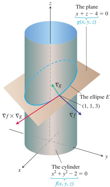
FIGURE 13.36 This cylinder and plane intersect in an ellipse E (Example 3).
Plane Tangent to a Surface
EXAMPLE 2 Find the plane tangent to the surface
Solution We calculate the partial derivatives of
The tangent plane is therefore
or
EXAMPLE 3 The surfaces
and
meet in an ellipse E (Figure 13.36). Find parametric equations for the line tangent to E at the point
Solution The tangent line is orthogonal to both
The tangent line to the ellipse of intersection is
Estimating Change in a Specific Direction
The directional derivative plays a role similar to that of an ordinary derivative when we want to estimate how much the value of a function f changes if we move a small distance ds from a point
For a function of two or more variables, we use the formula
Directional derivative
where u is the direction of the motion away from
Estimating the Change in f in a Direction u
To estimate the change in the value of a differentiable function f when we move a small distance ds from a point
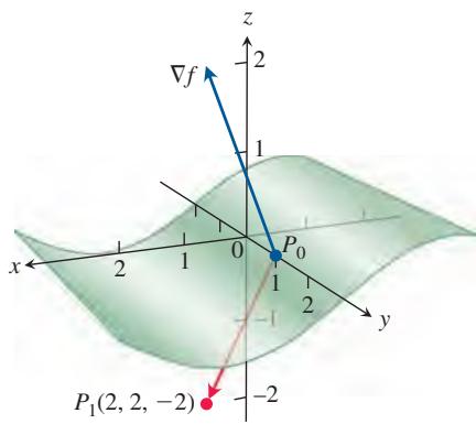
EXAMPLE 4 Estimate how much the value of
FIGURE 13.37 As
will change if the point
Solution We first find the derivative of
The gradient of
Therefore,
The change df in f that results from moving ds = 0.1 unit away from
See Figure 13.37.
How to Linearize a Function of Two Variables
Functions of two variables can be quite complicated, and we sometimes need to approximate them with simpler ones that give the accuracy required for specific applications without being so difficult to work with. We do this in a way that is similar to the way we find linear replacements for functions of a single variable (Section 3.11).
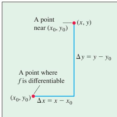
FIGURE 13.38 If f is differentiable at
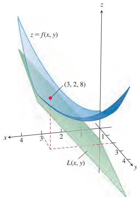
FIGURE 13.39 The tangent plane
Suppose the function we wish to approximate is
where
In other words, as long as
DEFINITIONS The linearization of a function
at a point 𝑓 ( 𝑥 , 𝑦 ) where ( 𝑥 0 , 𝑦 0 ) is differentiable is the function 𝑓 𝐿 ( 𝑥 , 𝑦 ) = 𝑓 ( 𝑥 0 , 𝑦 0 ) + 𝑓 𝑥 ( 𝑥 0 , 𝑦 0 ) ( 𝑥 − 𝑥 0 ) + 𝑓 𝑦 ( 𝑥 0 , 𝑦 0 ) ( 𝑦 − 𝑦 0 ) .
The approximation
is the standard linear approximation of
From Equation (3), we find that the plane
EXAMPLE 5 Find the linearization of
at the point (3, 2).
Solution We first evaluate
which yields
The linearization of
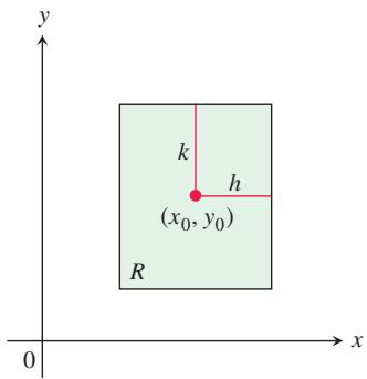
FIGURE 13.40 The rectangular region
When we approximate a differentiable function
If we can find a common upper bound M for
The Error in the Standard Linear Approximation
If
satisfies the inequality
To make
Differentials
Recall from Section 3.11 that for a function of a single variable,
and the differential of
We now consider the differential of a function of two variables.
Suppose a differentiable function
A straightforward calculation based on the definition of
The differentials dx and dy are independent variables, so they can be assigned any values. Often we take
DEFINITION If we move from
to a point ( 𝑥 0 , 𝑦 0 ) nearby, the resulting change ( 𝑥 0 + 𝑑 𝑥 , 𝑦 0 + 𝑑 𝑦 ) 𝑑 𝑓 = 𝑓 𝑥 ( 𝑥 0 , 𝑦 0 ) 𝑑 𝑥 + 𝑓 𝑦 ( 𝑥 0 , 𝑦 0 ) 𝑑 𝑦
in the linearization of f is called the total differential of f.
EXAMPLE 6 Suppose that a cylindrical can is designed to have a radius of 1 cm and a height of 5 cm, but that the radius and height are off by the amounts dr = +0.03 and dh = -0.1. Estimate the resulting absolute change in the volume of the can.
Solution To estimate the absolute change in
With
EXAMPLE 7 Your company manufactures stainless steel right circular cylindrical molasses storage tanks that are 2.5 m high with a radius of 0.5 m. How sensitive are the tanks’ volumes to small variations in height and radius?
Solution With
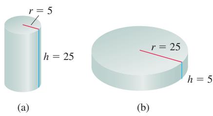
FIGURE 13.41 The volume of cylinder (a) is more sensitive to a small change in r than it is to an equally small change in h. The volume of cylinder (b) is more sensitive to small changes in h than it is to small changes in r (Example 7).
Thus, a 1-unit change in
In contrast, if the values of
Now the volume is more sensitive to changes in h than to changes in r (Figure 13.41).
The general rule is that functions are most sensitive to small changes in the variables that generate the largest partial derivatives.
Functions of More Than Two Variables
Analogous results hold for differentiable functions of more than two variables.
- The linearization of
𝑓 ( 𝑥 , 𝑦 , 𝑧 ) 𝑃 0 ( 𝑥 0 , 𝑦 0 , 𝑧 0 )
- Suppose that
𝑅 𝑃 0 𝑓 | 𝑓 𝑥 𝑥 | , | 𝑓 𝑦 𝑦 | , | 𝑓 𝑧 𝑧 | , | 𝑓 𝑥 𝑦 | , | 𝑓 𝑥 𝑧 | | 𝑓 𝑦 𝑧 | 𝑀 𝑅 𝐸 ( 𝑥 , 𝑦 , 𝑧 ) = 𝑓 ( 𝑥 , 𝑦 , 𝑧 ) − 𝐿 ( 𝑥 , 𝑦 , 𝑧 ) 𝑓 𝐿 𝑅
- If the second partial derivatives of
𝑓 𝑥 , 𝑦 , 𝑧 𝑥 0 , 𝑦 0 𝑧 0 𝑑 𝑥 , 𝑑 𝑦 𝑑 𝑧
gives a good approximation of the resulting change in f.
EXAMPLE 8 Find the linearization
at the point
Solution Routine calculations give
Thus,
Since
and
EXERCISES 13.6
Tangent Planes and Normal Lines to Surfaces In Exercises 1–10, find equations for the
(a) tangent plane and
(b) normal line at the point
-
𝑥 2 + 𝑦 2 − 𝑧 2 = 1 8 , 𝑃 0 ( 3 , 5 , − 4 ) -
2 𝑧 − 𝑥 2 = 0 , 𝑃 0 ( 2 , 0 , 2 ) -
𝑥 2 + 2 𝑥 𝑦 − 𝑦 2 + 𝑧 2 = 7 , 𝑃 0 ( 1 , − 1 , 3 ) -
c o s 𝜋 𝑥 − 𝑥 2 𝑦 + 𝑒 𝑥 𝑧 + 𝑦 𝑧 = 4 , 𝑃 0 ( 0 , 1 , 2 )
-
𝑥 l n 𝑦 + 𝑦 l n 𝑧 = 𝑥 , 𝑃 0 ( 1 , 1 , 𝑒 ) -
𝑦 𝑒 𝑥 + 𝑧 𝑒 𝑦 2 = 𝑧 , 𝑃 0 ( 0 , 0 , 1 )
In Exercises 11–14, find an equation for the plane that is tangent to the given surface at the given point.
-
𝑧 = l n ( 𝑥 2 + 𝑦 2 ) , ( 1 , 0 , 0 ) -
𝑧 = 𝑒 − ( 𝑥 2 + 𝑦 2 ) , ( 0 , 0 , 1 ) -
𝑧 = √ 𝑦 − 𝑥 -
𝑧 = 4 𝑥 2 + 𝑦 2 , ( 1 , 1 , 5 )
Tangent Lines to Intersecting Surfaces
In Exercises 15–20, find parametric equations for the line tangent to the curve of intersection of the surfaces at the given point.
-
Surfaces:
𝑥 𝑦 𝑧 = 1 𝑥 2 + 2 𝑦 2 + 3 𝑧 2 = 6 -
Surfaces:
𝑥 2 + 2 𝑦 + 2 𝑧 = 4 𝑦 = 1 -
Surfaces:
𝑥 + 𝑦 2 + 𝑧 = 2 𝑦 = 1 -
Surfaces:
𝑥 3 + 3 𝑥 2 𝑦 2 + 𝑦 3 + 4 𝑥 𝑦 − 𝑧 2 = 0 𝑥 2 + 𝑦 2 + 𝑧 2 = 1 1 -
Surfaces:
𝑥 2 + 𝑦 2 = 4 𝑥 2 + 𝑦 2 − 𝑧 = 0 ( √ 2 , √ 2 , 4 )
Estimating Change
- By about how much will
change if the point
- By about how much will
change as the point
- By about how much will
change if the point
- By about how much will
change if the point
- Temperature change along a circle Suppose that the Celsius temperature at the point
( 𝑥 , 𝑦 ) 𝑇 ( 𝑥 , 𝑦 ) = 𝑥 s i n 2 𝑦
a. How fast is the temperature experienced by the particle changing in degrees Celsius per meter at the point
b. How fast is the temperature experienced by the particle changing in degrees Celsius per second at P?
- Changing temperature along a space curve The Celsius temperature in a region in space is given by
𝑇 ( 𝑥 , 𝑦 , 𝑧 ) = 2 𝑥 2 − 𝑥 𝑦 𝑧 𝑥 = 2 𝑡 2 𝑧 = − 𝑡 2
a. How fast is the temperature experienced by the particle changing in degrees Celsius per meter when the particle is at the point
b. How fast is the temperature experienced by the particle changing in degrees Celsius per second at P?
Finding Linearizations
In Exercises 27–32, find the linearization
-
𝑓 ( 𝑥 , 𝑦 ) = 𝑥 2 + 𝑦 2 + 1 -
𝑓 ( 𝑥 , 𝑦 ) = ( 𝑥 + 𝑦 + 2 ) 2 ( 0 , 0 ) ( 1 , 2 ) -
𝑓 ( 𝑥 , 𝑦 ) = 3 𝑥 − 4 𝑦 + 5 -
𝑓 ( 𝑥 , 𝑦 ) = 𝑥 3 𝑦 4 ( 1 , 1 ) ( 0 , 0 ) -
𝑓 ( 𝑥 , 𝑦 ) = 𝑒 𝑥 c o s 𝑦 -
𝑓 ( 𝑥 , 𝑦 ) = 𝑒 2 𝑦 − 𝑥 ( 0 , 0 ) ( 1 , 2 ) -
Wind chill factor Wind chill, a measure of the apparent temperature felt on exposed skin, is a function of air temperature and wind speed. The precise formula, updated by the National Weather Service in 2001 and based on modern heat transfer theory, a human face model, and skin tissue resistance, is (after unit conversion)
where T is air temperature in
| 5 | 0 | -5 | -10 | -15 | -20 | -25 | |
| 10 | 2.7 | -3.3 | -9.3 | -15.2 | -21.2 | -27.2 | |
| 20 | 1.1 | -5.2 | -11.5 | -17.8 | -24.1 | -30.4 | |
| 30 | 0.1 | -6.4 | -13.0 | -19.5 | -26.0 | -32.5 | |
| 40 | -0.7 | -7.4 | -14.0 | -20.7 | -27.4 | -34.1 | |
| 50 | -1.3 | -8.1 | -14.9 | -21.7 | -28.5 | -35.4 | |
| 60 | -1.8 | -8.7 | -15.7 | -22.6 | -29.5 | -36.4 |
a. Use the table to find
b. Use the formula to find
c. Find the linearization
d. Use
iii)
- Find the linearization
𝐿 ( 𝑣 , 𝑇 ) 𝑊 ( 𝑣 , 𝑇 ) ( 5 0 , − 2 0 )
a.
b.
c.
Bounding the Error in Linear Approximations
In Exercises 35–40, find the linearization
𝑓 ( 𝑥 , 𝑦 ) = 𝑥 2 − 3 𝑥 𝑦 + 5 𝑃 0 ( 2 , 1 )
-
𝑓 ( 𝑥 , 𝑦 ) = ( 1 / 2 ) 𝑥 2 + 𝑥 𝑦 + ( 1 / 4 ) 𝑦 2 + 3 𝑥 − 3 𝑦 + 4 𝑃 0 ( 2 , 2 ) | 𝑥 − 2 | ≤ 0 . 1 | 𝑦 − 2 | ≤ 0 . 1 -
𝑓 ( 𝑥 , 𝑦 ) = 1 + 𝑦 + 𝑥 c o s 𝑦 𝑃 0 ( 0 , 0 )
(Use
𝑓 ( 𝑥 , 𝑦 ) = 𝑥 𝑦 2 + 𝑦 c o s ( 𝑥 − 1 ) 𝑃 0 ( 1 , 2 )
𝑓 ( 𝑥 , 𝑦 ) = 𝑒 𝑥 c o s 𝑦 𝑃 0 ( 0 , 0 )
(Use
𝑓 ( 𝑥 , 𝑦 ) = l n 𝑥 + l n 𝑦 𝑃 0 ( 1 , 1 )
Linearizations for Three Variables
Find the linearizations
𝑓 ( 𝑥 , 𝑦 , 𝑧 ) = 𝑥 𝑦 + 𝑦 𝑧 + 𝑥 𝑧 ( 1 , 1 , 1 ) ( 1 , 0 , 0 )
c.
𝑓 ( 𝑥 , 𝑦 , 𝑧 ) = 𝑥 2 + 𝑦 2 + 𝑧 2 ( 1 , 1 , 1 ) ( 0 , 1 , 0 )
c.
-
𝑓 ( 𝑥 , 𝑦 , 𝑧 ) = √ 𝑥 2 + 𝑦 2 + 𝑧 2 ( 1 , 0 , 0 ) ( 1 , 1 , 0 ) ( 1 , 2 , 2 ) -
𝑓 ( 𝑥 , 𝑦 , 𝑧 ) = ( s i n 𝑥 𝑦 ) / 𝑧 ( 𝜋 / 2 , 1 , 1 ) ( 2 , 0 , 1 ) -
𝑓 ( 𝑥 , 𝑦 , 𝑧 ) = 𝑒 𝑥 + c o s ( 𝑦 + 𝑧 ) ( 0 , 0 , 0 ) ( 0 , 𝜋 2 , 0 ) ( 0 , 𝜋 4 , 𝜋 4 ) -
𝑓 ( 𝑥 , 𝑦 , 𝑧 ) = t a n − 1 ( 𝑥 𝑦 𝑧 ) ( 1 , 0 , 0 ) ( 1 , 1 , 0 ) ( 1 , 1 , 1 )
In Exercises 47–50, find the linearization
𝑓 ( 𝑥 , 𝑦 , 𝑧 ) = 𝑥 𝑧 − 3 𝑦 𝑧 + 2 𝑃 0 ( 1 , 1 , 2 )
R:
-
𝑓 ( 𝑥 , 𝑦 , 𝑧 ) = 𝑥 𝑦 + 2 𝑦 𝑧 − 3 𝑥 𝑧 𝑃 0 ( 1 , 1 , 0 ) -
𝑓 ( 𝑥 , 𝑦 , 𝑧 ) = √ 2 c o s 𝑥 s i n ( 𝑦 + 𝑧 ) 𝑃 0 ( 0 , 0 , 𝜋 / 4 )
Estimating Error; Sensitivity to Change
-
Estimating maximum error Suppose that
𝑇 𝑇 = 𝑥 ( 𝑒 𝑦 + 𝑒 − 𝑦 ) 𝑥 𝑦 l n 2 | 𝑑 𝑥 | = 0 . 1 | 𝑑 𝑦 | = 0 . 0 2 𝑇 -
Variation in electrical resistance The resistance R produced by wiring resistors of
𝑅 1 𝑅 2
a. Show that
b. You have designed a two-resistor circuit, like the one shown, to have resistances of
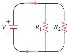
c. In another circuit like the one shown, you plan to change
-
You plan to calculate the area of a long, thin rectangle from measurements of its length and width. Which dimension should you measure more carefully? Give reasons for your answer.
-
a. Around the point
( 1 , 0 ) 𝑓 ( 𝑥 , 𝑦 ) = 𝑥 2 ( 𝑦 + 1 )
b. What ratio of dx to dy will make df equal zero at
- Value of a
2 × 2 | 𝑎 | | 𝑏 | , | 𝑐 | | 𝑑 | 𝑎 , 𝑏 , 𝑐 𝑑
most sensitive? Give reasons for your answer.
- The Wilson lot size formula The Wilson lot size formula in economics says that the most economical quantity Q of goods (radios, shoes, brooms, whatever) for a store to order is given by the formula
𝑄 = √ 2 𝐾 𝑀 / ℎ ( 𝐾 0 , 𝑀 0 , ℎ 0 ) = ( 2 , 2 0 , 0 . 0 5 )
Theory and Examples
- The linearization of
𝑓 ( 𝑥 , 𝑦 ) 𝑃 0 ( 𝑥 0 , 𝑦 0 , 𝑓 ( 𝑥 0 , 𝑦 0 ) ) 𝑧 = 𝑓 ( 𝑥 , 𝑦 ) 𝑓
or
Thus, the tangent plane at
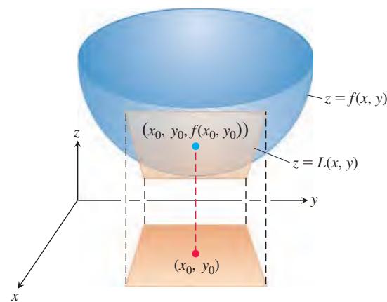
- Change along the involute of a circle Find the derivative of
𝑓 ( 𝑥 , 𝑦 ) = 𝑥 2 + 𝑦 2
is tangent to the surface
- Normal curves A smooth curve is normal to a surface
𝑓 ( 𝑥 , 𝑦 , 𝑧 ) = 𝑐 ∇ 𝑓
Show that the curve
is normal to the surface
- Consider a closed rectangular box with a square base, as shown in the figure. Assume x is measured with an error of at most 0.5% and y is measured with an error of at most 0.75%, so we have
| 𝑑 𝑥 | / 𝑥 < 0 . 0 0 5 | 𝑑 𝑦 | / 𝑦 < 0 . 0 0 7 5
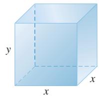
a. Use a differential to estimate the relative error
b. Use a differential to estimate the relative error
13.7 Extreme Values and Saddle Points
HISTORICAL BIOGRAPHY
Siméon-Denis Poisson
(1781-1840)
French mathematician Poisson studied with Lagrange and Laplace at the École polytechnique.and did so well that he was made an assistant professor upon his graduation. In 1806, he replaced Fourier as the professor of mathematics. Poisson’s early work in mechanics appeared in his first volume of
To know more, visit the companion Website.
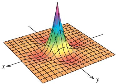
FIGURE 13.42 The function
has a maximum value of 1 and a minimum value of about -0.067 on the square region
Continuous functions of two variables assume extreme values on closed, bounded domains (see Figures 13.42 and 13.43). We see in this section that we can narrow the search for these extreme values by examining the functions’ first partial derivatives. A function of two variables can assume extreme values only at boundary points of the domain or at interior domain points where both first partial derivatives are zero or where one or both of the first partial derivatives fail to exist. However, the vanishing of derivatives at an interior point
Local Extreme Values for Functions of Two Variables
To find the local extreme values of a function of a single variable, we look for points where the graph has a horizontal tangent line. At such points, we then look for local maxima, local minima, and points of inflection. For a function
DEFINITIONS Let
be defined on a region 𝑓 ( 𝑥 , 𝑦 ) containing the point 𝑅 . Then ( 𝑎 , 𝑏 )
is a local maximum value of f if 𝑓 ( 𝑎 , 𝑏 ) for all domain points 𝑓 ( 𝑎 , 𝑏 ) ≥ 𝑓 ( 𝑥 , 𝑦 ) in an open disk centered at ( 𝑥 , 𝑦 ) . ( 𝑎 , 𝑏 ) is an absolute maximum value of f on R if 𝑓 ( 𝑎 , 𝑏 ) for all domain points 𝑓 ( 𝑎 , 𝑏 ) ≥ 𝑓 ( 𝑥 , 𝑦 ) in R. ( 𝑥 , 𝑦 )
is a local minimum value of f if 𝑓 ( 𝑎 , 𝑏 ) for all domain points 𝑓 ( 𝑎 , 𝑏 ) ≤ 𝑓 ( 𝑥 , 𝑦 ) in an open disk centered at ( 𝑥 , 𝑦 ) . ( 𝑎 , 𝑏 ) is an absolute minimum value of f on R if 𝑓 ( 𝑎 , 𝑏 ) for all domain points 𝑓 ( 𝑎 , 𝑏 ) ≤ 𝑓 ( 𝑥 , 𝑦 ) in R. ( 𝑥 , 𝑦 )
FIGURE 13.43 The “roof surface”
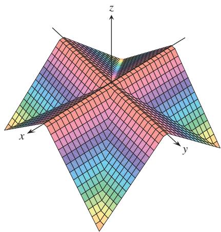
has a maximum value of 0 and a minimum value of -a on the square region
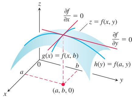
FIGURE 13.45 If a local maximum of f occurs at x = a, y = b, then the first partial derivatives
Local maxima correspond to mountain peaks on the surface
As with functions of a single variable, the key to identifying the local extrema is the First Derivative Theorem, which we next state and prove.
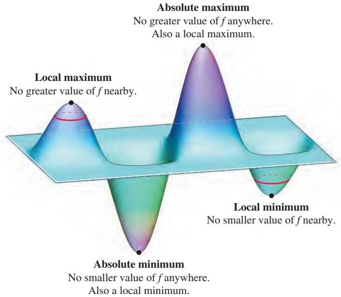
FIGURE 13.44 A local maximum occurs at a mountain peak, and a local minimum occurs at a valley low point.
THEOREM 10—First Derivative Theorem for Local Extreme Values
If
Proof If
If we substitute the values
for the tangent plane to the surface
Thus, Theorem 10 says that the surface does indeed have a horizontal tangent plane at a local extremum, provided there is a tangent plane there.
DEFINITION An interior point of the domain of a function
where both 𝑓 ( 𝑥 , 𝑦 ) and 𝑓 𝑥 are zero or where one or both of 𝑓 𝑦 and 𝑓 𝑥 do not exist is a critical point of f. 𝑓 𝑦
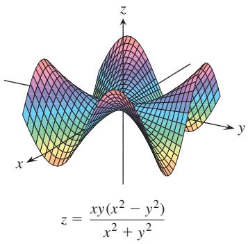
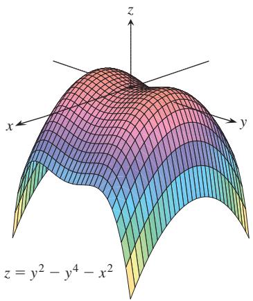
FIGURE 13.46 Saddle points at the origin.
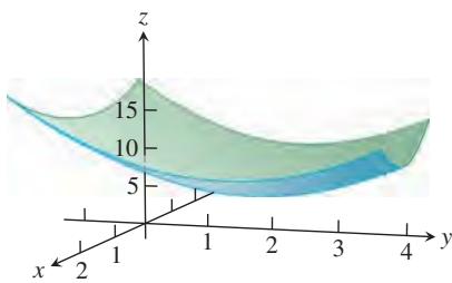
FIGURE 13.47 The graph of the function
Theorem 10 says that the only points where a function
DEFINITION A differentiable function
has a saddle point at a critical point 𝑓 ( 𝑥 , 𝑦 ) if in every open disk centered at ( 𝑎 , 𝑏 ) there are domain points ( 𝑎 , 𝑏 ) where ( 𝑥 , 𝑦 ) and domain points 𝑓 ( 𝑥 , 𝑦 ) > 𝑓 ( 𝑎 , 𝑏 ) where ( 𝑥 , 𝑦 ) . The corresponding point 𝑓 ( 𝑥 , 𝑦 ) < 𝑓 ( 𝑎 , 𝑏 ) on the surface ( 𝑎 , 𝑏 , 𝑓 ( 𝑎 , 𝑏 ) ) is called a saddle point of the surface (Figure 13.46). 𝑧 = 𝑓 ( 𝑥 , 𝑦 )
EXAMPLE 1 Find the local extreme values of
Solution The domain of f is the entire plane (so there are no boundary points) and the partial derivatives
The only possibility is the point
EXAMPLE 2 Find the local extreme values (if any) of
Solution The domain of f is the entire plane (so there are no boundary points) and the partial derivatives
That
THEOREM 11—Second Derivative Test for Local Extreme Values
Suppose that
i)
ii)
iii)
iv) the test is inconclusive at
The expression
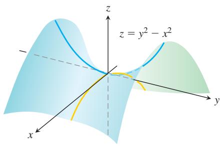
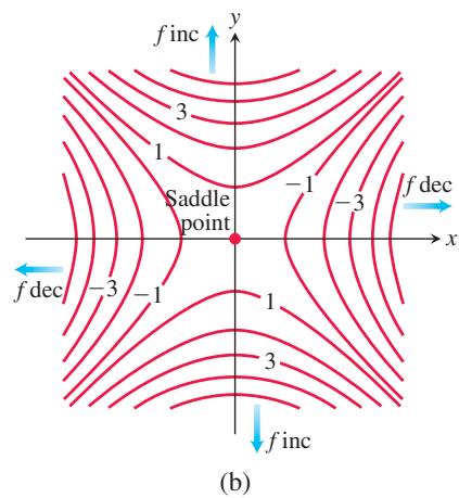
FIGURE 13.48 (a) The origin is a saddle point of the function
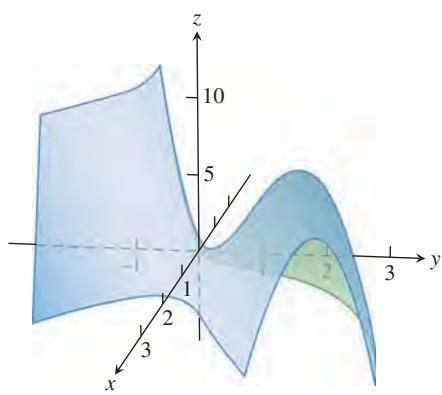
FIGURE 13.49 The surface
The discriminant is the determinant of the Hessian matrix of f,
Note that by Theorem 2, we have
Theorem 11 says that if the discriminant is positive at the point
EXAMPLE 3 Find the local extreme values of the function
Solution The function is defined and differentiable for all x and y, and its domain has no boundary points. The function therefore has extreme values only at the points where
or
Therefore, the point
The discriminant of
The combination
tells us that
EXAMPLE 4 Find the local extreme values of
Solution Since f is differentiable everywhere, it can assume extreme values only where
From the first of these equations we find
The two critical points are therefore
To classify the critical points, we calculate the second derivatives:
The discriminant is given by
At the critical point
EXAMPLE 5 Find the critical points of the function
Solution First we find the partial derivatives
Since both partial derivatives are continuous everywhere, the only critical points are
Next we calculate the second partial derivatives in order to evaluate the discriminant at each critical point:
The following table summarizes the values needed by the Second Derivative Test.
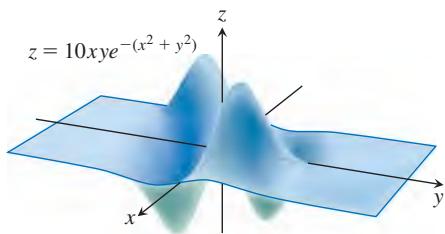
FIGURE 13.50 A graph of the function in Example 5.
| Critical Point | Discriminant D | |||
| (0,0) | 0 | 10 | 0 | -100 |
| 0 | ||||
| 0 | ||||
| 0 | ||||
| 0 |
From the table we find that D < 0 at the critical point
Absolute Maxima and Minima on Closed Bounded Regions
We organize the search for the absolute extrema of a continuous function
-
List the interior points of R where f may have local maxima and minima and evaluate f at these points. These are the critical points of f.
-
List the boundary points of
𝑅 𝑓 𝑓 -
Look through the lists for the maximum and minimum values of f. These will be the absolute maximum and minimum values of f on R.
(b)
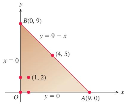
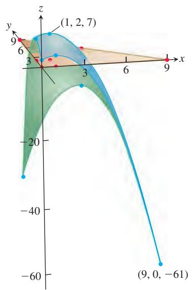
FIGURE 13.51 (a) This triangular region is the domain of the function in Example 6. (b) The graph of the function in Example 6. The blue points are the candidates for maxima or minima.
EXAMPLE 6 Find the absolute maximum and minimum values of
on the triangular region in the first quadrant bounded by the lines x = 0, y = 0, and y = 9 - x.
Solution Since f is differentiable, the only places where f can assume these values are points inside the triangle where
(a) Interior points. For these we have
yielding the single point
(b) Boundary points. We take the triangle one side at a time:
i) On the segment OA we always have y = 0. Therefore, we can regard
for
or at the interior points where
ii) On the segment OB we always have x = 0. Therefore, on this segment we can regard
on the closed interval [0, 9]. Its extreme values can occur at the endpoints or at interior points where
iii) We have already accounted for the values of
Setting
At this value of
Summary We list all the function value candidates: 7, 2, -61, 3, -43, 6, -11. The maximum is 7, which
Solving extreme value problems with algebraic constraints on the variables usually requires the method of Lagrange multipliers, which is introduced in the next section. But sometimes we can solve such problems directly, as in the next example.
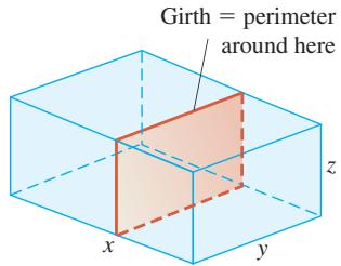
FIGURE 13.52 The box in Example 7.
EXAMPLE 7 A delivery company accepts only rectangular boxes the sum of whose length and girth (perimeter of a cross-section) does not exceed 270 cm. Find the dimensions of an acceptable box of largest volume.
Solution Let x, y, and z represent the length, width, and height of the rectangular box, respectively. Then the girth is
Setting the first partial derivatives equal to zero,
gives the critical points
Then
Thus,
and
so (45,45) gives a maximum volume. The dimensions of the package are
Despite the power of Theorem 11, we urge you to remember its limitations. It does not apply to boundary points of a function’s domain, where it is possible for a function to have extreme values along with nonzero derivatives. Also, it does not apply to points where either
Summary of Max-Min Tests
The extreme values of
Finding maximum and minimum values for functions of more than two variables is an important problem with many important applications, from machine learning to making economic predictions. The problem becomes much harder as the number of variables increases. The process of finding extrema for functions with high-dimensional domains is discussed in Appendices B.2 and B.3.
EXERCISES 13.7
Finding Local Extrema
Find all the local maxima, local minima, and saddle points of the functions in Exercises 1–30.
-
𝑓 ( 𝑥 , 𝑦 ) = 𝑥 2 + 𝑥 𝑦 + 𝑦 2 + 3 𝑥 − 3 𝑦 + 4 -
𝑓 ( 𝑥 , 𝑦 ) = 2 𝑥 𝑦 − 5 𝑥 2 − 2 𝑦 2 + 4 𝑥 + 4 𝑦 − 4 -
𝑓 ( 𝑥 , 𝑦 ) = 𝑥 2 + 𝑥 𝑦 + 3 𝑥 + 2 𝑦 + 5
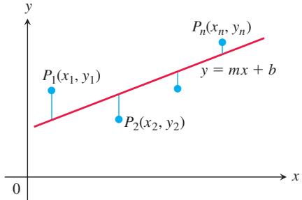
𝑓 ( 𝑥 , 𝑦 ) = 5 𝑥 𝑦 − 7 𝑥 2 + 3 𝑥 − 6 𝑦 + 2
-
𝑓 ( 𝑥 , 𝑦 ) = 2 𝑥 2 + 3 𝑥 𝑦 + 4 𝑦 2 − 5 𝑥 + 2 𝑦 -
𝑓 ( 𝑥 , 𝑦 ) = 𝑥 2 − 2 𝑥 𝑦 + 2 𝑦 2 − 2 𝑥 + 2 𝑦 + 1 -
𝑓 ( 𝑥 , 𝑦 ) = 𝑥 2 − 𝑦 2 − 2 𝑥 + 4 𝑦 + 6 -
𝑓 ( 𝑥 , 𝑦 ) = 𝑥 2 + 2 𝑥 𝑦 -
𝑓 ( 𝑥 , 𝑦 ) = √ 5 6 𝑥 2 − 8 𝑦 2 − 1 6 𝑥 − 3 1 + 1 − 8 𝑥 -
𝑓 ( 𝑥 , 𝑦 ) = 1 − 3 √ 𝑥 2 + 𝑦 2 -
𝑓 ( 𝑥 , 𝑦 ) = 𝑥 3 − 𝑦 3 − 2 𝑥 𝑦 + 6 -
𝑓 ( 𝑥 , 𝑦 ) = 𝑥 3 + 3 𝑥 𝑦 + 𝑦 3 -
𝑓 ( 𝑥 , 𝑦 ) = 6 𝑥 2 − 2 𝑥 3 + 3 𝑦 2 + 6 𝑥 𝑦 -
𝑓 ( 𝑥 , 𝑦 ) = 𝑥 3 + 𝑦 3 + 3 𝑥 2 − 3 𝑦 2 − 8 -
𝑓 ( 𝑥 , 𝑦 ) = 𝑥 3 + 3 𝑥 𝑦 2 − 1 5 𝑥 + 𝑦 3 − 1 5 𝑦 -
𝑓 ( 𝑥 , 𝑦 ) = 2 𝑥 3 + 2 𝑦 3 − 9 𝑥 2 + 3 𝑦 2 − 1 2 𝑦 -
𝑓 ( 𝑥 , 𝑦 ) = 4 𝑥 𝑦 − 𝑥 4 − 𝑦 4 -
𝑓 ( 𝑥 , 𝑦 ) = 𝑥 4 + 𝑦 4 + 4 𝑥 𝑦 -
𝑓 ( 𝑥 , 𝑦 ) = 1 𝑥 2 + 𝑦 2 − 1 2 2 . 𝑓 ( 𝑥 , 𝑦 ) = 1 𝑥 + 𝑥 𝑦 + 1 𝑦 -
𝑓 ( 𝑥 , 𝑦 ) = 𝑦 s i n 𝑥 2 4 . 𝑓 ( 𝑥 , 𝑦 ) = 𝑒 2 𝑥 c o s 𝑦 -
𝑓 ( 𝑥 , 𝑦 ) = 𝑒 𝑥 2 + 𝑦 2 − 4 𝑥 2 6 . 𝑓 ( 𝑥 , 𝑦 ) = 𝑒 𝑦 − 𝑦 𝑒 𝑥 -
𝑓 ( 𝑥 , 𝑦 ) = 𝑒 − 𝑦 ( 𝑥 2 + 𝑦 2 ) 2 8 . 𝑓 ( 𝑥 , 𝑦 ) = 𝑒 𝑥 ( 𝑥 2 − 𝑦 2 ) -
𝑓 ( 𝑥 , 𝑦 ) = 2 l n 𝑥 + l n 𝑦 − 4 𝑥 − 𝑦 -
𝑓 ( 𝑥 , 𝑦 ) = l n ( 𝑥 + 𝑦 ) + 𝑥 2 − 𝑦
Finding Absolute Extrema
In Exercises 31–38, find the absolute maxima and minima of the functions on the given domains.
-
𝑓 ( 𝑥 , 𝑦 ) = 2 𝑥 2 − 4 𝑥 + 𝑦 2 − 4 𝑦 + 1 -
𝐷 ( 𝑥 , 𝑦 ) = 𝑥 2 − 𝑥 𝑦 + 𝑦 2 + 1 𝑥 = 0 , 𝑦 = 4 , 𝑦 = 𝑥 -
𝑓 ( 𝑥 , 𝑦 ) = 𝑥 2 + 𝑦 2 𝑥 = 0 , 𝑦 = 0 , 𝑦 + 2 𝑥 = 2 -
𝑇 ( 𝑥 , 𝑦 ) = 𝑥 2 + 𝑥 𝑦 + 𝑦 2 − 6 𝑥 0 ≤ 𝑥 ≤ 5 , − 3 ≤ 𝑦 ≤ 3 -
𝑇 ( 𝑥 , 𝑦 ) = 𝑥 2 + 𝑥 𝑦 + 𝑦 2 − 6 𝑥 + 2 0 ≤ 𝑥 ≤ 5 , − 3 ≤ 𝑦 ≤ 0 -
𝑓 ( 𝑥 , 𝑦 ) = 4 8 𝑥 𝑦 − 3 2 𝑥 3 − 2 4 𝑦 2 0 ≤ 𝑥 ≤ 1 , 0 ≤ 𝑦 ≤ 1 -
𝑓 ( 𝑥 , 𝑦 ) = ( 4 𝑥 − 𝑥 2 ) c o s 𝑦 1 ≤ 𝑥 ≤ 3 , − 𝜋 / 4 ≤ 𝑦 ≤ 𝜋 / 4 -
𝑓 ( 𝑥 , 𝑦 ) = 4 𝑥 − 8 𝑥 𝑦 + 2 𝑦 + 1 𝑥 = 0 , 𝑦 = 0 , 𝑥 + 𝑦 = 1 -
Find two numbers
𝑎 𝑏 𝑎 ≤ 𝑏
has its largest value.
- Find two numbers
𝑎 𝑏 𝑎 ≤ 𝑏
has its largest value.
- Temperatures A flat circular plate has the shape of the region
𝑥 2 + 𝑦 2 ≤ 1 𝑥 2 + 𝑦 2 = 1 ( 𝑥 , 𝑦 )
Find the temperatures at the hottest and coldest points on the plate.
- Find the critical point of
in the open first quadrant
Theory and Examples
- Find the maxima, minima, and saddle points of
𝑓 ( 𝑥 , 𝑦 )
Describe your reasoning in each case.
- The discriminant
𝑓 𝑥 𝑥 𝑓 𝑦 𝑦 − 𝑓 2 𝑥 𝑦 𝑧 = 𝑓 ( 𝑥 , 𝑦 )
-
Show that
( 0 , 0 ) 𝑓 ( 𝑥 , 𝑦 ) = 𝑥 2 + 𝑘 𝑥 𝑦 + 𝑦 2 𝑘 ≠ 0 -
For what values of the constant k does the Second Derivative Test guarantee that
𝑓 ( 𝑥 , 𝑦 ) = 𝑥 2 + 𝑘 𝑥 𝑦 + 𝑦 2 ( 0 , 0 ) ( 0 , 0 ) -
If
𝑓 𝑥 ( 𝑎 , 𝑏 ) = 𝑓 𝑦 ( 𝑎 , 𝑏 ) = 0 ( 𝑎 , 𝑏 ) -
Can you conclude anything about
𝑓 ( 𝑎 , 𝑏 ) ( 𝑎 , 𝑏 ) 𝑓 𝑥 𝑥 ( 𝑎 , 𝑏 ) 𝑓 𝑦 𝑦 ( 𝑎 , 𝑏 ) -
Among all the points on the graph of
𝑧 = 1 0 − 𝑥 2 − 𝑦 2 𝑥 + 2 𝑦 + 3 𝑧 = 0 -
Find the point on the graph of
𝑧 = 𝑥 2 + 𝑦 2 + 1 0 𝑥 + 2 𝑦 − 𝑧 = 0 -
Find the point on the plane
3 𝑥 + 2 𝑦 + 𝑧 = 6 -
Find the minimum distance from the point
( 2 , − 1 , 1 ) 𝑥 + 𝑦 − 𝑧 = 2 -
Find three numbers whose sum is 9 and whose sum of squares is a minimum.
-
Find three positive numbers whose sum is 3 and whose product is a maximum.
-
Find the maximum value of
𝑠 = 𝑥 𝑦 + 𝑦 𝑧 + 𝑥 𝑧 𝑥 + 𝑦 + 𝑧 = 6 -
Find the minimum distance from the cone
𝑧 = √ 𝑥 2 + 𝑦 2 ( − 6 , 4 , 0 ) -
Find the dimensions of the rectangular box of maximum volume that can be inscribed inside the sphere
𝑥 2 + 𝑦 2 + 𝑧 2 = 4 -
Among all closed rectangular boxes of volume
2 7 𝑐 𝑚 3 -
You are to construct an open rectangular box from
1 2 𝑚 2 -
Consider the function
𝑓 ( 𝑥 , 𝑦 ) = 𝑥 2 + 𝑦 2 + 2 𝑥 𝑦 − 𝑥 − 𝑦 + 1 0 ≤ 𝑥 ≤ 1 0 ≤ 𝑦 ≤ 1
a. Show that
b. Find the absolute maximum value of f over the square.
-
Find the point on the graph of
𝑦 2 − 𝑥 𝑧 2 = 4 -
A rectangular box is inscribed in the region in the first octant bounded above by the plane with x-intercept 6, y-intercept 6, and z-intercept 6.
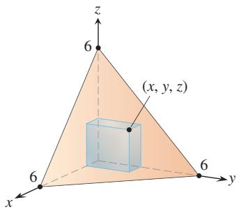
a. Find an equation for the plane.
b. Find the dimensions of the box of maximum volume.
Extreme Values on Parametrized Curves To find the extreme values of a function
a. The critical points (points where
In Exercises 63–66, find the absolute maximum and minimum values of the following functions on the given curves.
- Functions:
a.
a.
- Function:
𝑓 ( 𝑥 , 𝑦 ) = 𝑥 𝑦 𝑥 = 2 𝑡 𝑦 = 𝑡 + 1 𝑥 = 2 𝑡 𝑦 = 𝑡 + 1 − 1 ≤ 𝑡 ≤ 0 𝑥 = 2 𝑡 𝑦 = 𝑡 + 1 0 ≤ 𝑡 ≤ 1
- Functions:
ii) The line segment x = t, y = 2 - 2t,
- Least squares and regression lines When we try to fit a line
𝑦 = 𝑚 𝑥 + 𝑏 ( 𝑥 1 , 𝑦 1 ) , ( 𝑥 2 , 𝑦 2 ) , … , ( 𝑥 𝑛 , 𝑦 𝑛 )
(See the accompanying figure.) Show that the values of
with all sums running from k = 1 to k = n. Many scientific calculators have these formulas built in, enabling you to find m and b with only a few keystrokes after you have entered the data.
The line
- summarize data with a simple expression,
- predict values of y for other, experimentally untried values of x,
- handle data analytically.
In Exercises 68–70, use Equations (2) and (3) to find the least squares line for each set of data points. Then use the linear equation you obtain to predict the value of y that would correspond to x = 4.
-
( − 2 , 0 ) , ( 0 , 2 ) , ( 2 , 3 ) -
( − 1 , 2 ) , ( 0 , 1 ) , ( 3 , − 4 ) -
( 0 , 0 ) , ( 1 , 2 ) , ( 2 , 3 )
COMPUTER EXPLORATIONS
In Exercises 71–76, you will explore functions to identify their local extrema. Use a CAS to perform the following steps:
a. Plot the function over the given rectangle.
b. Plot some level curves in the rectangle.
c. Calculate the function’s first partial derivatives and use the CAS equation solver to find the critical points. How are the critical points related to the level curves plotted in part (b)? Which critical points, if any, appear to give a saddle point? Give reasons for your answer.
d. Calculate the function’s second partial derivatives and find the discriminant
e. Using the max-min tests, classify the critical points found in part (c). Are your findings consistent with your discussion in part (c)?
-
𝑓 ( 𝑥 , 𝑦 ) = 𝑥 4 + 𝑦 2 − 8 𝑥 2 − 6 𝑦 + 1 6 , − 3 ≤ 𝑥 ≤ 3 , − 6 ≤ 𝑦 ≤ 6 -
𝑓 ( 𝑥 , 𝑦 ) = 2 𝑥 4 + 𝑦 4 − 2 𝑥 2 − 2 𝑦 2 + 3 , − 3 / 2 ≤ 𝑥 ≤ 3 / 2 , − 3 / 2 ≤ 𝑦 ≤ 3 / 2 -
𝑓 ( 𝑥 , 𝑦 ) = 5 𝑥 6 + 1 8 𝑥 5 − 3 0 𝑥 4 + 3 0 𝑥 𝑦 2 − 1 2 0 𝑥 3 , − 4 ≤ 𝑥 ≤ 3 , − 2 ≤ 𝑦 ≤ 2
13.8 Lagrange Multipliers
HISTORICAL BIOGRAPHY
Joseph Louis Lagrange (1736–1813)
Lagrange was born in Turin, Italy. He enjoyed studying mathematics, despite his father’s wish that he study law. Lagrange’s mathematical contributions began as early as 1754 with the discovery of the calculus of variations and continued with applications to mechanics in 1756.
To know more, visit the companion Website.
Sometimes we need to find the extreme values of a function whose domain is constrained to lie within some particular subset of the plane—for example, a disk, a closed triangular region, or along a curve. We saw an instance of this situation in Example 6 of the previous section. Here we explore a powerful method for finding extreme values of constrained functions: the method of Lagrange multipliers.
Constrained Maxima and Minima
To gain some insight, we first consider a problem where a constrained minimum can be found by eliminating a variable.
EXAMPLE 1 Find the point
Solution The problem asks us to find the minimum value of the function
subject to the constraint that
Since
has a minimum value, we may solve the problem by finding the minimum value of
our problem reduces to finding the points
has its minimum value or values. Since the domain of h is the entire xy-plane, the First Derivative Theorem of Section 13.7 tells us that any minima that h might have must occur at points where
This leads to
which has the solution
We may apply a geometric argument together with the Second Derivative Test to show that these values minimize h. The z-coordinate of the corresponding point on the plane
Therefore, the point we seek is
The distance from P to the origin is
Attempts to solve a constrained maximum or minimum problem by substitution, as we might call the method of Example 1, do not always go smoothly.
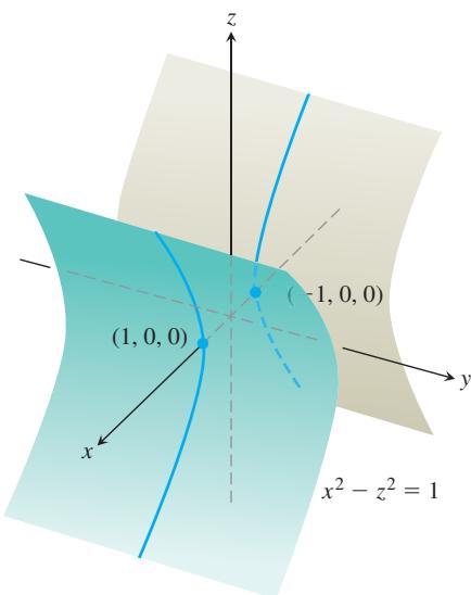
FIGURE 13.53 The hyperbolic cylinder
EXAMPLE 2 Find the points on the hyperbolic cylinder
Solution 1 The cylinder is shown in Figure 13.53. We seek the points on the cylinder closest to the origin. These are the points whose coordinates minimize the value of the function
subject to the constraint that
and the values of
To find the points on the cylinder whose coordinates minimize f, we look for the points in the xy-plane whose coordinates minimize h. The only extreme value of h occurs where
The hyperbolic cylinder
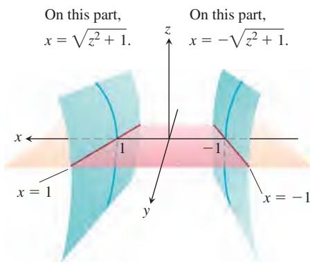
FIGURE 13.54 The region in the xy-plane from which the first two coordinates of the points
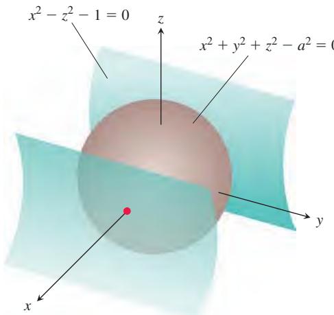
FIGURE 13.55 A sphere expanding like a soap bubble centered at the origin until it just touches the hyperbolic cylinder
that is, at the point
What happened is that the First Derivative Theorem found (as it should have) the point in the domain of h where h has a minimum value. We, on the other hand, want the points on the cylinder where h has a minimum value. Although the domain of h is the entire xy-plane, the domain from which we can select the first two coordinates of the points
We can avoid this problem if we treat y and z as independent variables (instead of x and y) and express x in terms of y and z as
With this substitution,
and we look for the points where k takes on its smallest value. The domain of k in the yz-plane now matches the domain from which we select the y- and z-coordinates of the points
or where
The corresponding points on the cylinder are
that the points
Solution 2 Another way to find the points on the cylinder closest to the origin is to imagine a small sphere centered at the origin expanding like a soap bubble until it just touches the cylinder (Figure 13.55). At each point of contact, the cylinder and sphere have the same tangent plane and normal line. Therefore, if the sphere and cylinder are represented as the level surfaces obtained by setting
equal to 0, then the gradients
or
Thus, the coordinates x, y, and z of any point of tangency will have to satisfy the three scalar equations
For what values of
For
What points on the surface
The points on the cylinder closest to the origin are the points
The Method of Lagrange Multipliers
In Solution 2 of Example 2, we used the method of Lagrange multipliers. The method says that the local extreme values of a function
for some scalar
To explore the method further and see why it works, we first make the following observation, which we state as a theorem.
THEOREM 12—The Orthogonal Gradient Theorem
Suppose that
Proof The values of
At any point
By dropping the z-terms in Theorem 12, we obtain a similar result for functions of two variables.
COROLLARY At the points on a smooth curve
Theorem 12 is the key to the method of Lagrange multipliers. Suppose that
FIGURE 13.56 Example 3 shows how to find the largest and smallest values of the product
The Method of Lagrange Multipliers
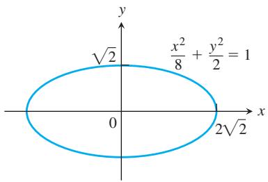
Suppose that
If they exist, absolute extrema can be found by comparing these values of f at each critical point satisfying Equation (1). For functions of two independent variables, the condition is similar, but without the variable z.
Some care must be used in applying this method. An extreme value may not actually exist (Exercise 45).
EXAMPLE 3 Find the largest and smallest values that the function
takes on the ellipse (Figure 13.56)
Solution We want to find the extreme values of
To do so, we first find the values of x, y, and
The gradient equation in Equations (1) gives
from which we find
and
so that
We now consider these two cases.
Case 1: If
Case 2: If
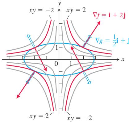
FIGURE 13.57 When subjected to the constraint
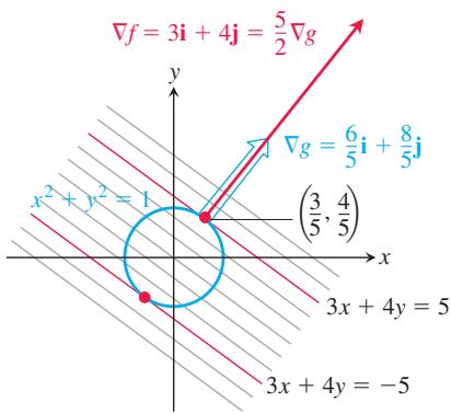
FIGURE 13.58 The function
The function
The Geometry of the Solution The level curves of the function
At the point
EXAMPLE 4 Find the maximum and minimum values of the function
Solution We model this as a Lagrange multiplier problem with
and look for the values of
The gradient equation implies that
These equations tell us, among other things, that
SO
Thus,
and
By calculating the value of
The Geometry of the Solution The level curves of
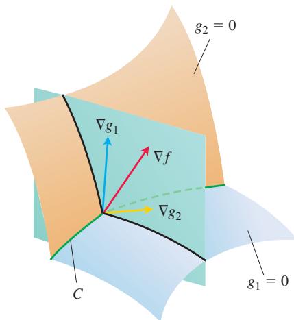
FIGURE 13.59 The vectors
also lies on the circle
Lagrange Multipliers with Two Constraints
Many problems require us to find the extreme values of a differentiable function
and
Equations (2) have a nice geometric interpretation. The surfaces
EXAMPLE 5 The plane
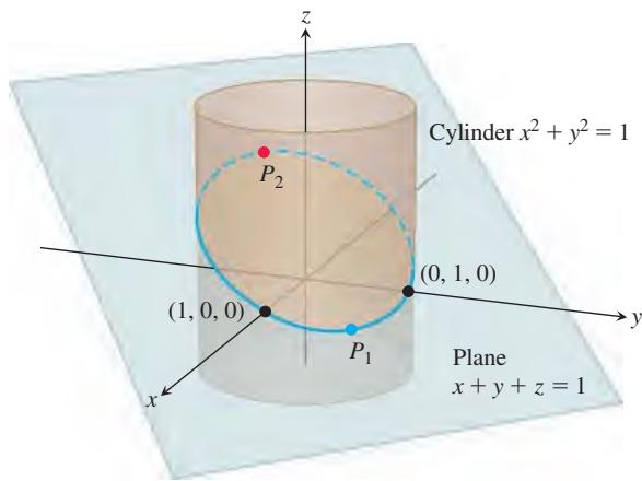
FIGURE 13.60 On the ellipse where the plane and cylinder meet, we find the points closest to and farthest from the origin (Example 5).
Solution We find the extreme values of
(the square of the distance from
The gradient equation in Equations (2) then gives
or
The scalar equations in Equations (5) yield
Equations (6) are satisfied simultaneously if either
In the first case, where z = 0, solving Equations (3) and (4) simultaneously to find the corresponding points on the ellipse gives the two points
In the second case, where
The corresponding points on the ellipse are
To find the points at maximum and minimum distance from the origin, we evaluate
The largest and smallest of these give the absolute extrema. Since
we see that the absolute minimum value of
The points on the ellipse closest to the origin are
EXERCISES 13.8
Two Independent Variables with One Constraint
-
Extrema on an ellipse Find the points on the ellipse
𝑥 2 + 2 𝑦 2 = 1 𝑓 ( 𝑥 , 𝑦 ) = 𝑥 𝑦 -
Extrema on a circle Find the extreme values of
𝑓 ( 𝑥 , 𝑦 ) = 𝑥 𝑦 𝑔 ( 𝑥 , 𝑦 ) = 𝑥 2 + 𝑦 2 − 1 0 = 0 -
Maximum on a line Find the maximum value of
𝑓 ( 𝑥 , 𝑦 ) = 4 9 − 𝑥 2 − 𝑦 2 𝑥 + 3 𝑦 = 1 0 -
Extrema on a line Find the local extreme values of
𝑓 ( 𝑥 , 𝑦 ) = 𝑥 2 𝑦 𝑥 + 𝑦 = 3 -
Constrained minimum Find the points on the curve
𝑥 𝑦 2 = 5 4 -
Constrained minimum Find the points on the curve
𝑥 2 𝑦 = 2 -
Use the method of Lagrange multipliers to find
a. Minimum on a hyperbola The minimum value of
b. Maximum on a line The maximum value of xy, subject to the constraint
Comment on the geometry of each solution.
-
Extrema on a curve Find the points on the curve
𝑥 2 + 𝑥 𝑦 + 𝑦 2 = 1 -
Minimum surface area with fixed volume Find the dimensions of the closed right circular cylindrical can of smallest surface area whose volume is
1 6 𝜋 𝑐 𝑚 3 -
Cylinder in a sphere Find the radius and height of the open right circular cylinder of largest surface area that can be inscribed in a sphere of radius
𝑎 -
Rectangle of greatest area in an ellipse Use the method of Lagrange multipliers to find the dimensions of the rectangle of greatest area that can be inscribed in the ellipse
𝑥 2 / 1 6 + 𝑦 2 / 9 = 1 -
Rectangle of longest perimeter in an ellipse Find the dimensions of the rectangle of largest perimeter that can be inscribed in the ellipse
𝑥 2 / 𝑎 2 + 𝑦 2 / 𝑏 2 = 1 -
Extrema on a circle Find the maximum and minimum values of
𝑥 2 + 𝑦 2 𝑥 2 − 2 𝑥 + 𝑦 2 − 4 𝑦 = 0 -
Extrema on a circle Find the maximum and minimum values of
3 𝑥 − 𝑦 + 6 𝑥 2 + 𝑦 2 = 4 -
Ant on a metal plate The temperature at a point
( 𝑥 , 𝑦 ) 𝑇 ( 𝑥 , 𝑦 ) = 4 𝑥 2 − 4 𝑥 𝑦 + 𝑦 2 -
Cheapest storage tank Your firm has been asked to design a storage tank for liquid petroleum gas. The customer’s specifications call for a cylindrical tank with hemispherical ends, and the tank is to hold
8 0 0 0 m 3
Three Independent Variables with One Constraint
-
Minimum distance to a point Find the point on the plane
𝑥 + 2 𝑦 + 3 𝑧 = 1 3 ( 1 , 1 , 1 ) -
Maximum distance to a point Find the point on the sphere
𝑥 2 + 𝑦 2 + 𝑧 2 = 4 ( 1 , − 1 , 1 ) -
Minimum distance to the origin Find the minimum distance from the surface
𝑥 2 − 𝑦 2 − 𝑧 2 = 1 -
Minimum distance to the origin Find the point on the surface
𝑧 = 𝑥 𝑦 + 1 -
Minimum distance to the origin Find the points on the surface
𝑧 2 = 𝑥 𝑦 + 4 -
Minimum distance to the origin Find the point(s) on the surface xyz = 1 closest to the origin.
-
Extrema on a sphere Find the maximum and minimum values of
on the sphere
-
Extrema on a sphere Find the points on the sphere
𝑥 2 + 𝑦 2 + 𝑧 2 = 2 5 𝑓 ( 𝑥 , 𝑦 , 𝑧 ) = 𝑥 + 2 𝑦 + 3 𝑧 -
Minimizing a sum of squares Find three real numbers whose sum is 9 and the sum of whose squares is as small as possible.
-
Maximizing a product Find the largest product the positive numbers x, y, and z can have if
𝑥 + 𝑦 + 𝑧 2 = 1 6 -
Rectangular box of largest volume in a sphere Find the dimensions of the closed rectangular box with maximum volume that can be inscribed in the unit sphere.
-
Box with vertex on a plane Find the volume of the largest closed rectangular box in the first octant having three faces in the coordinate planes and a vertex on the plane
𝑥 / 𝑎 + 𝑦 / 𝑏 + 𝑧 / 𝑐 = 1 𝑎 > 0 𝑏 > 0 𝑐 > 0 -
Hottest point on a space probe A space probe in the shape of the ellipsoid
enters Earth’s atmosphere and its surface begins to heat. After 1 hour, the temperature at the point
Find the hottest point on the probe’s surface.
-
Extreme temperatures on a sphere Suppose that the Celsius temperature at the point
( 𝑥 , 𝑦 , 𝑧 ) 𝑥 2 + 𝑦 2 + 𝑧 2 = 1 𝑇 = 4 0 0 𝑥 𝑦 𝑧 2 -
Cobb–Douglas production function During the 1920s, Charles Cobb and Paul Douglas modeled total production output P (of a firm, industry, or entire economy) as a function of labor hours involved x and capital invested y (which includes the monetary worth of all buildings and equipment). The Cobb–Douglas production function is given by
where k and
a. Show that a doubling of both labor and capital results in a doubling of production P.
b. Suppose a particular firm has the production function for
- (Continuation of Exercise 31.) If the cost of a unit of labor is
𝑐 1 𝑐 2 𝐵 𝑃 𝑐 1 𝑥 + 𝑐 2 𝑦 = 𝐵
- Maximizing a utility function: an example from economics In economics, the usefulness or utility of amounts
𝑥 𝑦 𝐺 1 𝐺 2 𝑈 ( 𝑥 , 𝑦 ) 𝐺 1 𝐺 2 𝑈 ( 𝑥 , 𝑦 ) 𝐺 1 𝑎 𝐺 2 𝑏 𝐺 1 𝐺 2 𝑐 𝑈 ( 𝑥 , 𝑦 ) 𝑎 𝑥 + 𝑏 𝑦 = 𝑐
Suppose that
and that the equation
Find the maximum value of U and the corresponding values of x and y subject to this latter constraint.
- Blood types Human blood types are classified by three gene forms A, B, and O. Blood types AA, BB, and OO are homozygous, and blood types AB, AO, and BO are heterozygous. If p, q, and r represent the proportions of the three gene forms to the population, respectively, then the Hardy–Weinberg Law asserts that the proportion Q of heterozygous persons in any specific population is modeled by
subject to
- Length of a beam In Section 4.6, Exercise 47, we posed a problem of finding the length L of the shortest beam that can reach over a wall of height h to a tall building located k units from the wall. Use Lagrange multipliers to show that
- Locating a radio telescope You are in charge of erecting a radio telescope on a newly discovered planet. To minimize interference, you want to place it where the magnetic field of the planet is weakest. The planet is spherical, with a radius of 6 units. Based on a coordinate system whose origin is at the center of the planet, the strength of the magnetic field is given by
𝑀 ( 𝑥 , 𝑦 , 𝑧 ) = 6 𝑥 − 𝑦 2 + 𝑥 𝑧 + 6 0
Extreme Values Subject to Two Constraints
-
Maximize the function
𝑓 ( 𝑥 , 𝑦 , 𝑧 ) = 𝑥 2 + 2 𝑦 − 𝑧 2 𝑦 + 𝑧 = 0 -
Minimize the function
𝑓 ( 𝑥 , 𝑦 , 𝑧 ) = 𝑥 2 + 𝑦 2 + 𝑧 2 𝑥 + 2 𝑦 + 3 𝑧 = 6 𝑥 + 3 𝑦 + 9 𝑧 = 9 -
Minimum distance to the origin Find the point closest to the origin on the line of intersection of the planes
𝑦 + 2 𝑧 = 1 2 𝑥 + 𝑦 = 6 -
Find the extreme values of
𝑓 ( 𝑥 , 𝑦 , 𝑧 ) = 2 𝑥 2 + 𝑦 𝑧 𝑥 2 + 𝑧 2 = 9 𝑦 − 𝑧 = 4 -
Extrema on a curve of intersection Find the extreme values of
𝑓 ( 𝑥 , 𝑦 , 𝑧 ) = 𝑥 2 𝑦 𝑧 + 1 𝑧 = 1 𝑥 2 + 𝑦 2 + 𝑧 2 = 1 0 -
a. Maximum on line of intersection Find the maximum value of w = xyz on the line of intersection of the two planes
𝑥 + 𝑦 + 𝑧 = 4 0 𝑥 + 𝑦 − 𝑧 = 0
b. Give a geometric argument to support your claim that you have found a maximum, and not a minimum, value of w.
-
Extrema on a circle of intersection Find the extreme values of the function
𝑓 ( 𝑥 , 𝑦 , 𝑧 ) = 𝑥 𝑦 + 𝑧 2 𝑥 2 + 𝑦 2 + 𝑧 2 = 4 -
Minimum distance to the origin Find the point closest to the origin on the curve of intersection of the plane
2 𝑦 + 4 𝑧 = 5 𝑧 2 = 4 𝑥 2 + 4 𝑦 2
Theory and Examples
-
The condition
∇ 𝑓 = 𝜆 ∇ 𝑔 ∇ 𝑓 = 𝜆 ∇ 𝑔 𝑓 ( 𝑥 , 𝑦 ) 𝑔 ( 𝑥 , 𝑦 ) = 0 ∇ 𝑔 ≠ 0 𝑓 ( 𝑥 , 𝑦 ) = 𝑥 + 𝑦 𝑥 + 𝑦 𝑓 ( 𝑥 , 𝑦 ) = 𝑥 + 𝑦 -
A least squares plane The plane
𝑧 = 𝐴 𝑥 + 𝐵 𝑦 + 𝐶 ( 𝑥 𝑘 , 𝑦 𝑘 , 𝑧 𝑘 )
Find the values of A, B, and C that minimize
the sum of the squares of the deviations.
- a. Maximum on a sphere Show that the maximum value of
𝑎 2 𝑏 2 𝑐 2 𝑟 ( 𝑟 2 / 3 ) 3
b. Geometric and arithmetic means Using part (a), show that for nonnegative numbers
that is, the geometric mean of three nonnegative numbers is less than or equal to their arithmetic mean.
- Sum of products Let
𝑎 1 , 𝑎 2 , … , 𝑎 𝑛 ∑ 𝑛 𝑖 = 1 𝑎 𝑖 𝑥 𝑖 ∑ 𝑛 𝑖 = 1 𝑥 2 𝑖 = 1
COMPUTER EXPLORATIONS
In Exercises 49–54, use a CAS to perform the following steps implementing the method of Lagrange multipliers for finding constrained extrema:
a. Form the function
b. Determine all the first partial derivatives of
c. Solve the system of equations found in part (b) for all the unknowns, including
d. Evaluate f at each of the solution points found in part (c), and select the extreme value subject to the constraints asked for in the exercise.
-
Minimize
𝑓 ( 𝑥 , 𝑦 , 𝑧 ) = 𝑥 𝑦 + 𝑦 𝑧 𝑥 2 + 𝑦 2 − 2 = 0 𝑥 2 + 𝑧 2 − 2 = 0 -
Minimize
𝑓 ( 𝑥 , 𝑦 , 𝑧 ) = 𝑥 𝑦 𝑧 𝑥 2 + 𝑦 2 − 1 = 0 -
Maximize
𝑓 ( 𝑥 , 𝑦 , 𝑧 ) = 𝑥 2 + 𝑦 2 + 𝑧 2 2 𝑦 + 4 𝑧 − 5 = 0 4 𝑥 2 + 4 𝑦 2 − 𝑧 2 = 0 -
Minimize
𝑓 ( 𝑥 , 𝑦 , 𝑧 ) = 𝑥 2 + 𝑦 2 + 𝑧 2 𝑥 2 − 𝑥 𝑦 + 𝑦 2 − 𝑧 2 − 1 = 0 𝑥 2 + 𝑦 2 − 1 = 0 -
Minimize
𝑓 ( 𝑥 , 𝑦 , 𝑧 , 𝑤 ) = 𝑥 2 + 𝑦 2 + 𝑧 2 + 𝑤 2 2 𝑥 − 𝑦 + 𝑧 − 𝑤 − 1 = 0 𝑥 + 𝑦 − 𝑧 + 𝑤 − 1 = 0 -
Determine the distance from the line
𝑦 = 𝑥 + 1 𝑦 2 = 𝑥 ( 𝑥 , 𝑦 ) ( 𝑤 , 𝑧 ) ( 𝑥 − 𝑤 ) 2 + ( 𝑦 − 𝑧 ) 2
13.9 Taylor’s Formula for Two Variables
In this section we use Taylor’s formula to derive the Second Derivative Test for local extreme values (Section 13.7) and the error formula for linearizations of functions of two independent variables (Section 13.6). The use of Taylor’s formula in these derivations leads to an extension of the formula that provides polynomial approximations of all orders for functions of two independent variables.
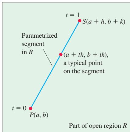
Derivation of the Second Derivative Test
FIGURE 13.61 We begin the derivation of the Second Derivative Test at
Let
If
Since
Since
for some c between 0 and 1. Writing Equation (1) in terms of f gives
Since
To determine whether
Now, if
from the signs of
From Equation (5) we see that
-
If
𝑓 𝑥 𝑥 < 0 𝑓 𝑥 𝑥 𝑓 𝑦 𝑦 − 𝑓 2 𝑥 𝑦 > 0 ( 𝑎 , 𝑏 ) 𝑄 ( 0 ) < 0 ℎ 𝑘 𝑓 ( 𝑎 , 𝑏 ) -
If
𝑓 𝑥 𝑥 > 0 𝑓 𝑥 𝑥 𝑓 𝑦 𝑦 − 𝑓 2 𝑥 𝑦 > 0 ( 𝑎 , 𝑏 ) 𝑄 ( 0 ) > 0 ℎ 𝑘 𝑓 ( 𝑎 , 𝑏 ) -
If
𝑓 𝑥 𝑥 𝑓 𝑦 𝑦 − 𝑓 2 𝑥 𝑦 < 0 ( 𝑎 , 𝑏 ) 𝑄 ( 0 ) > 0 𝑄 ( 0 ) < 0 𝑃 0 ( 𝑎 , 𝑏 , 𝑓 ( 𝑎 , 𝑏 ) ) 𝑧 = 𝑓 ( 𝑥 , 𝑦 ) 𝑃 0 𝑃 0 ( 𝑎 , 𝑏 ) -
If
𝑓 𝑥 𝑥 𝑓 𝑦 𝑦 − 𝑓 2 𝑥 𝑦 = 0 𝑄 ( 0 ) 𝑄 ( 𝑐 )
The Error Formula for Linear Approximations
We want to show that the difference
The function
The inequality we want comes from Equation (2). We substitute
This equation reveals that
Hence, if
Taylor’s Formula for Functions of Two Variables
The formulas derived earlier for
These are the first two instances of a more general formula,
which says that applying
to
If the partial derivatives of
and take t = 1 to obtain
When we replace the first n derivatives on the right of this last series by their equivalent expressions from Equation (6) evaluated at t = 0 and add the appropriate remainder term, we arrive at the following formula.
Taylor’s Formula for
Suppose
The first n derivative terms are evaluated at
If
Taylor’s Formula for
The first n derivative terms are evaluated at
Taylor’s formula provides polynomial approximations of two-variable functions. The first
EXAMPLE 1 Find a quadratic approximation to
Solution We take n = 2 in Equation (8):
Calculating the values of the partial derivatives,
we have the result
The error in the approximation is
The third derivatives never exceed 1 in absolute value because they are products of sines and cosines. Also,
(rounded up). The error will not exceed 0.00134 if
Exercises 13.9
Finding Quadratic and Cubic Approximations
In Exercises 1–10, use Taylor’s formula for
-
𝑓 ( 𝑥 , 𝑦 ) = 𝑥 𝑒 𝑦 -
𝑓 ( 𝑥 , 𝑦 ) = 𝑒 𝑥 c o s 𝑦 -
𝑓 ( 𝑥 , 𝑦 ) = 𝑦 s i n 𝑥 -
𝑓 ( 𝑥 , 𝑦 ) = s i n 𝑥 c o s 𝑦 -
𝑓 ( 𝑥 , 𝑦 ) = 𝑒 𝑥 l n ( 1 + 𝑦 ) -
𝑓 ( 𝑥 , 𝑦 ) = l n ( 2 𝑥 + 𝑦 + 1 ) -
𝑓 ( 𝑥 , 𝑦 ) = s i n ( 𝑥 2 + 𝑦 2 ) -
𝑓 ( 𝑥 , 𝑦 ) = c o s ( 𝑥 2 + 𝑦 2 )
-
Use Taylor’s formula to find a quadratic approximation of
𝑓 ( 𝑥 , 𝑦 ) = c o s 𝑥 c o s 𝑦 | 𝑥 | ≤ 0 . 1 | 𝑦 | ≤ 0 . 1 -
Use Taylor’s formula to find a quadratic approximation of
𝑒 𝑥 s i n 𝑦 | 𝑥 | ≤ 0 . 1 | 𝑦 | ≤ 0 . 1
13.10 Partial Derivatives with Constrained Variables
In finding partial derivatives of functions like
and fail to be independent. In this section we learn how to find partial derivatives in situations like this, which occur in economics, engineering, and physics.
Decide Which Variables Are Dependent and Which Are Independent
If the variables in a function
Solution We are given two equations in the four unknowns x, y, z, and w. Like many such systems, this one can be solved for two of the unknowns (the dependent variables) in terms of the others (the independent variables). In being asked for
Dependent Independent
In either case, we can express w explicitly in terms of the selected independent variables. We do this by using the second equation
In the first case, the remaining dependent variable is
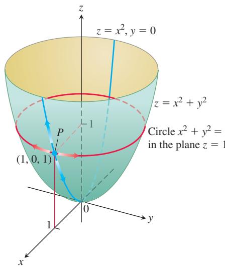
FIGURE 13.62 If P is constrained to lie on the paraboloid
and therefore
This is the formula for
In the second case, where the independent variables are x and z and the remaining dependent variable is y, we eliminate the dependent variable y in the expression for w by replacing
and therefore
This is the formula for
The formulas for
The geometric interpretations of Equations (1) and (2) help to explain why the equations differ. The function
If we take
At the point
If we take x and z to be independent, then we find
as we found in our second solution.
How to Find 𝜕 𝑤 / 𝜕 𝑥 𝑤 = 𝑓 ( 𝑥 , 𝑦 , 𝑧 )
As we saw in Example 1, a typical routine for finding
-
Decide which variables are to be dependent and which are to be independent. (In practice, the decision is based on the physical or theoretical context of our work. In the exercises at the end of this section, we say which variables are which.)
-
Eliminate the other dependent variable(s) in the expression for w.
-
Differentiate as usual.
If we cannot carry out Step 2 after deciding which variables are dependent, we differentiate the equations as they are and try to solve for
EXAMPLE 2 Find
and x and y are the independent variables.
Solution It is not convenient to eliminate z in the expression for w. We therefore differentiate both equations implicitly with respect to x, treating x and y as independent variables and w and z as dependent variables. This gives
and
These equations may now be combined to express
and substitute into Equation (3) to get
The value of this derivative at
HISTORICAL BIOGRAPHY
Sonya Kovalevsky (1850–1891)
Kovalevsky, a Russian mathematician, primarily worked on the theory of partial differential equations, and a central result on the existence of solutions still bears her name. She published numerous papers on partial differential equations, eventually gaining recognition as the first woman to be elected a member of the Russian Imperial Academy of Sciences in 1889.
To know more, visit the companion Website.
Notation
To show what variables are assumed to be independent in calculating a derivative, we can use the following notation:
Solution With x, y, z independent, we have
Arrow Diagrams
In solving problems like the one in Example 3, it often helps to start with an arrow diagram that shows how the variables and functions are related. If
and we are asked to find
To avoid confusion between the independent and intermediate variables with the same symbolic names in the diagram, it is helpful to rename the intermediate variables (so they are seen as functions of the independent variables). Thus, let u = x, v = y, and s = z denote the renamed intermediate variables. With this notation, the arrow diagram becomes
The diagram shows the independent variables on the left, the intermediate variables and their relation to the independent variables in the middle, and the dependent variable on the right. The function w now becomes
where
To find
EXERCISES 13.10
Finding Partial Derivatives with Constrained Variables
In Exercises 1–3, begin by drawing a diagram that shows the relations among the variables.
-
If
𝑤 = 𝑥 2 + 𝑦 2 + 𝑧 2 𝑧 = 𝑥 2 + 𝑦 2 ( 𝜕 𝑤 𝜕 𝑦 ) 𝑧 ( 𝜕 𝑤 𝜕 𝑧 ) 𝑥 ( 𝜕 𝑤 𝜕 𝑧 ) 𝑦 -
If
𝑤 = 𝑥 2 + 𝑦 − 𝑧 + s i n 𝑡 𝑥 + 𝑦 = 𝑡 ( 𝜕 𝑤 𝜕 𝑦 ) 𝑥 , 𝑧 ( 𝜕 𝑤 𝜕 𝑦 ) 𝑧 , 𝑡 ( 𝜕 𝑤 𝜕 𝑧 ) 𝑥 , 𝑦 ( 𝜕 𝑤 𝜕 𝑧 ) 𝑦 , 𝑡 ( 𝜕 𝑤 𝜕 𝑡 ) 𝑥 , 𝑧 ( 𝜕 𝑤 𝜕 𝑡 ) 𝑦 , 𝑧 -
Let
𝑈 = 𝑓 ( 𝑃 , 𝑉 , 𝑇 ) 𝑃 𝑉 = 𝑛 𝑅 𝑇 𝑛 𝑅 ( 𝜕 𝑈 𝜕 𝑃 ) 𝑉 ( 𝜕 𝑈 𝜕 𝑇 ) 𝑉
Show that the equations
each give
-
Find a.
( 𝜕 𝑤 𝜕 𝑥 ) 𝑦 ( 𝜕 𝑤 𝜕 𝑧 ) 𝑦 ( 𝑥 , 𝑦 , 𝑧 ) = ( 0 , 1 , 𝜋 ) 𝑤 = 𝑥 2 + 𝑦 2 + 𝑧 2 𝑦 s i n 𝑧 + 𝑧 s i n 𝑥 = 0 -
Find a.
( 𝜕 𝑤 𝜕 𝑦 ) 𝑥 ( 𝜕 𝑤 𝜕 𝑦 ) 𝑧 ( 𝑤 , 𝑥 , 𝑦 , 𝑧 ) = ( 4 , 2 , 1 , − 1 ) 𝑤 = 𝑥 2 𝑦 2 + 𝑦 𝑧 − 𝑧 3 𝑥 2 + 𝑦 2 + 𝑧 2 = 6 -
Find
( 𝜕 𝑢 / 𝜕 𝑦 ) 𝑥 ( 𝑢 , 𝑣 ) = ( √ 2 , 1 ) 𝑥 = 𝑢 2 + 𝑣 2 𝑦 = 𝑢 𝑣 -
Suppose that
𝑥 2 + 𝑦 2 = 𝑟 2 𝑥 = 𝑟 c o s 𝜃
- Suppose that
𝑤 = 𝑥 2 − 𝑦 2 + 4 𝑧 + 𝑡 𝑥 + 2 𝑧 + 𝑡 = 2 5
Theory and Examples
- Establish the fact, widely used in hydrodynamics, that if
𝑓 ( 𝑥 , 𝑦 , 𝑧 ) = 0
(Hint: Express all the derivatives in terms of the formal partial derivatives
- If
𝑧 = 𝑥 + 𝑓 ( 𝑢 ) 𝑢 = 𝑥 𝑦
- Suppose that the equation
𝑔 ( 𝑥 , 𝑦 , 𝑧 ) = 0 𝑧 𝑥 𝑦 𝑔 𝑧 ≠ 0
- Suppose that
𝑓 ( 𝑥 , 𝑦 , 𝑧 , 𝑤 ) = 0 𝑔 ( 𝑥 , 𝑦 , 𝑧 , 𝑤 ) = 0 𝑧 𝑤 𝑥 𝑦
Show that
and
CHAPTER 13 Questions to Guide Your Review
-
What is a real-valued function of two independent variables? Three independent variables? Give examples.
-
What does it mean for sets in the plane or in space to be open? Closed? Give examples. Give examples of sets that are neither open nor closed.
-
How can you display the values of a function
𝑓 ( 𝑥 , 𝑦 ) 𝑓 ( 𝑥 , 𝑦 , 𝑧 ) -
What does it mean for a function
𝑓 ( 𝑥 , 𝑦 ) 𝐿 ( 𝑥 , 𝑦 ) → ( 𝑥 0 , 𝑦 0 ) -
When is a function of two (three) independent variables continuous at a point in its domain? Give examples of functions that are continuous at some points but not others.
-
What can be said about algebraic combinations and compositions of continuous functions?
-
Explain the two-path test for nonexistence of limits.
-
How are the partial derivatives
𝜕 𝑓 / 𝜕 𝑥 𝜕 𝑓 / 𝜕 𝑦 𝑓 ( 𝑥 , 𝑦 ) -
How does the relation between first partial derivatives and continuity of functions of two independent variables differ from the relation between first derivatives and continuity for real-valued functions of a single independent variable? Give an example.
-
What is the Mixed Derivative Theorem for mixed second-order partial derivatives? How can it help in calculating partial derivatives of second and higher orders? Give examples.
-
What does it mean for a function
𝑓 ( 𝑥 , 𝑦 ) -
How can you sometimes decide from examining
𝑓 𝑥 𝑓 𝑦 𝑓 ( 𝑥 , 𝑦 ) -
What is the general Chain Rule? What form does it take for functions of two independent variables? Three independent variables? Functions defined on surfaces? How do you diagram these different forms? Give examples. What pattern enables one to remember all the different forms?
-
What is the derivative of a function
𝑓 ( 𝑥 , 𝑦 ) 𝑃 0 -
What is the gradient vector of a differentiable function
𝑓 ( 𝑥 , 𝑦 ) -
How do you find the tangent line at a point on a level curve of a differentiable function
𝑓 ( 𝑥 , 𝑦 )
plane and normal line at a point on a level surface of a differentiable function
-
How can you use directional derivatives to estimate change?
-
How do you linearize a function
𝑓 ( 𝑥 , 𝑦 ) ( 𝑥 0 , 𝑦 0 ) -
What can you say about the accuracy of linear approximations of functions of two (three) independent variables?
-
If
( 𝑥 , 𝑦 ) ( 𝑥 0 , 𝑦 0 ) ( 𝑥 0 + 𝑑 𝑥 , 𝑦 0 + 𝑑 𝑦 ) 𝑓 ( 𝑥 , 𝑦 ) -
How do you define local maxima, local minima, and saddle points for a differentiable function
𝑓 ( 𝑥 , 𝑦 ) -
What derivative tests are available for determining the local extreme values of a function
𝑓 ( 𝑥 , 𝑦 ) -
How do you find the extrema of a continuous function
𝑓 ( 𝑥 , 𝑦 ) 𝑥 𝑦 -
Describe the method of Lagrange multipliers and give examples.
-
How does Taylor’s formula for a function
𝑓 ( 𝑥 , 𝑦 ) -
If
𝑤 = 𝑓 ( 𝑥 , 𝑦 , 𝑧 ) 𝑔 ( 𝑥 , 𝑦 , 𝑧 ) = 0 ( 𝜕 𝑤 / 𝜕 𝑥 ) 𝑦
CHAPTER 13 Practice Exercises
Domain, Range, and Level Curves
In Exercises 1–4, find the domain and range of the given function and identify its level curves. Sketch a typical level curve.
-
𝑓 ( 𝑥 , 𝑦 ) = 9 𝑥 2 + 𝑦 2 -
𝑓 ( 𝑥 , 𝑦 ) = 𝑒 𝑥 + 𝑦 -
𝑔 ( 𝑥 , 𝑦 ) = 1 / 𝑥 𝑦 -
𝑔 ( 𝑥 , 𝑦 ) = √ 𝑥 2 − 𝑦
In Exercises 5–8, find the domain and range of the given function and identify its level surfaces. Sketch a typical level surface.
-
𝑓 ( 𝑥 , 𝑦 , 𝑧 ) = 𝑥 2 + 𝑦 2 − 𝑧 -
𝑔 ( 𝑥 , 𝑦 , 𝑧 ) = 𝑥 2 + 4 𝑦 2 + 9 𝑧 2 -
ℎ ( 𝑥 , 𝑦 , 𝑧 ) = 1 𝑥 2 + 𝑦 2 + 𝑧 2 -
𝑘 ( 𝑥 , 𝑦 , 𝑧 ) = 1 𝑥 2 + 𝑦 2 + 𝑧 2 + 1
Evaluating Limits
Find the limits in Exercises 9–14.
-
l i m ( 𝑥 , 𝑦 ) → ( 𝜋 , l n 2 ) 𝑒 𝑦 c o s 𝑥 -
l i m ( 𝑥 , 𝑦 ) → ( 0 , 0 ) 2 + 𝑦 𝑥 + c o s 𝑦 -
l i m ( 𝑥 , 𝑦 ) → ( 1 , 1 ) 𝑥 − 𝑦 𝑥 2 − 𝑦 2 -
l i m ( 𝑥 , 𝑦 ) → ( 1 , 1 ) 𝑥 3 𝑦 3 − 1 𝑥 𝑦 − 1 -
l i m 𝑃 → ( 1 , − 1 , 𝑒 ) l n | 𝑥 + 𝑦 + 𝑧 | -
l i m 𝑃 → ( 1 , − 1 , − 1 ) a r c t a n ( 𝑥 + 𝑦 + 𝑧 )
By considering different paths of approach, show that the limits in Exercises 15 and 16 do not exist.
-
l i m ( 𝑥 , 𝑦 ) → ( 0 , 0 ) 𝑦 ≠ 𝑥 2 𝑦 𝑥 2 − 𝑦 -
l i m ( 𝑥 , 𝑦 ) → ( 0 , 0 ) 𝑥 𝑦 ≠ 0 𝑥 2 + 𝑦 2 𝑥 𝑦 -
Continuous extension Let
𝑓 ( 𝑥 , 𝑦 ) = ( 𝑥 2 − 𝑦 2 ) / ( 𝑥 2 + 𝑦 2 ) ( 𝑥 , 𝑦 ) ≠ ( 0 , 0 ) 𝑓 ( 0 , 0 ) 𝑓 -
Continuous extension Let
Is
Partial Derivatives
In Exercises 19–24, find the partial derivative of the function with respect to each variable.
-
𝑔 ( 𝑟 , 𝜃 ) = 𝑟 c o s 𝜃 + 𝑟 s i n 𝜃 -
𝑓 ( 𝑥 , 𝑦 ) = 1 2 l n ( 𝑥 2 + 𝑦 2 ) + a r c t a n 𝑦 𝑥 -
𝑓 ( 𝑅 1 , 𝑅 2 , 𝑅 3 ) = 1 𝑅 1 + 1 𝑅 2 + 1 𝑅 3 -
ℎ ( 𝑥 , 𝑦 , 𝑧 ) = s i n ( 2 𝜋 𝑥 + 𝑦 − 3 𝑧 ) -
𝑃 ( 𝑛 , 𝑅 , 𝑇 , 𝑉 ) = 𝑛 𝑅 𝑇 𝑉 -
𝑓 ( 𝑟 , 𝑙 , 𝑇 , 𝑤 ) = 1 2 𝑟 𝑙 √ 𝑇 𝜋 𝑤
Second-Order Partials
Find the second-order partial derivatives of the functions in Exercises 25–28.
-
𝑔 ( 𝑥 , 𝑦 ) = 𝑦 + 𝑥 𝑦 -
𝑔 ( 𝑥 , 𝑦 ) = 𝑒 𝑥 + 𝑦 s i n 𝑥 -
𝑓 ( 𝑥 , 𝑦 ) = 𝑥 + 𝑥 𝑦 − 5 𝑥 3 + l n ( 𝑥 2 + 1 ) -
𝑓 ( 𝑥 , 𝑦 ) = 𝑦 2 − 3 𝑥 𝑦 + c o s 𝑦 + 7 𝑒 𝑦
Chain Rule Calculations
-
Find
𝑑 𝑤 / 𝑑 𝑡 𝑡 = 0 𝑤 = s i n ( 𝑥 𝑦 + 𝜋 ) 𝑥 = 𝑒 𝑡 𝑦 = l n ( 𝑡 + 1 ) -
Find
𝑑 𝑤 / 𝑑 𝑡 𝑡 = 1 𝑤 = 𝑥 𝑒 𝑦 + 𝑦 s i n 𝑧 − c o s 𝑧 𝑥 = 2 √ 𝑡 𝑦 = 𝑡 − 1 + l n 𝑡 𝑧 = 𝜋 𝑡 -
Find
𝜕 𝑤 / 𝜕 𝑟 𝜕 𝑤 / 𝜕 𝑠 𝑟 = 𝜋 𝑠 = 0 𝑤 = s i n ( 2 𝑥 − 𝑦 ) , 𝑥 = 𝑟 + s i n 𝑠 , 𝑦 = 𝑟 𝑠 -
Find
𝜕 𝑤 / 𝜕 𝑢 𝜕 𝑥 𝜕 𝑤 / 𝜕 𝑣 𝜕 𝑥 𝑢 = 𝑣 = 0 𝑤 = l n √ 1 + 𝑥 2 − t a n − 1 𝑥 𝑥 = 2 𝑒 𝑢 c o s 𝑣 -
Find the value of the derivative of
𝑓 ( 𝑥 , 𝑦 , 𝑧 ) = 𝑥 𝑦 + 𝑦 𝑧 + 𝑥 𝑧 𝑥 = c o s 𝑡 𝑦 = s i n 𝑡 𝑧 = c o s 2 𝑡 -
Show that if
𝑤 = 𝑓 ( 𝑠 ) 𝑠 𝑠 = 𝑦 + 5 𝑥
Implicit Differentiation
Assuming that the equations in Exercises 35 and 36 define
2 𝑥 𝑦 + 𝑒 𝑥 + 𝑦 − 2 = 0 , 𝑃 ( 0 , l n 2 )
Directional Derivatives
In Exercises 37–40, find the directions in which f increases and decreases most rapidly at
-
𝑓 ( 𝑥 , 𝑦 ) = c o s 𝑥 c o s 𝑦 , 𝑃 0 ( 𝜋 / 4 , 𝜋 / 4 ) , 𝐯 = 3 𝐢 + 4 𝐣 -
𝑓 ( 𝑥 , 𝑦 ) = 𝑥 2 𝑒 − 2 𝑦 , 𝑃 0 ( 1 , 0 ) , 𝐯 = 𝐢 + 𝐣 -
𝑓 ( 𝑥 , 𝑦 , 𝑧 ) = l n ( 2 𝑥 + 3 𝑦 + 6 𝑧 ) 𝑃 0 ( − 1 , − 1 , 1 )
- Derivative in velocity direction Find the derivative of
𝑓 ( 𝑥 , 𝑦 , 𝑧 ) = 𝑥 𝑦 𝑧
at
-
Maximum directional derivative What is the largest value that the directional derivative of
𝑓 ( 𝑥 , 𝑦 , 𝑧 ) = 𝑥 𝑦 𝑧 -
Directional derivatives with given values At the point
( 1 , 2 ) 𝑓 ( 𝑥 , 𝑦 ) ( 2 , 2 ) ( 1 , 1 )
a. Find
b. Find the derivative of
- Which of the following statements are true if
𝑓 ( 𝑥 , 𝑦 ) ( 𝑥 0 , 𝑦 0 )
a. If
b. The derivative of f at
c. The directional derivative of
d. At
Gradients, Tangent Planes, and Normal Lines
In Exercises 45 and 46, sketch the surface
In Exercises 47 and 48, find an equation for the plane tangent to the level surface
In Exercises 49 and 50, find an equation for the plane tangent to the surface
𝑧 = 1 / ( 𝑥 2 + 𝑦 2 ) , ( 1 , 1 , 1 / 2 )
In Exercises 51 and 52, find equations for the lines that are tangent and normal to the level curve
-
𝑦 − s i n 𝑥 = 1 , 𝑃 0 ( 𝜋 , 1 ) -
𝑦 2 2 − 𝑥 2 2 = 3 2 , 𝑃 0 ( 1 , 2 )
Tangent Lines to Curves
In Exercises 53 and 54, find parametric equations for the line that is tangent to the curve of intersection of the surfaces at the given point.
- Surfaces:
𝑥 2 + 2 𝑦 + 2 𝑧 = 4 , 𝑦 = 1
Point:
- Surfaces:
𝑥 + 𝑦 2 + 𝑧 = 2
Point:
Linearizations
In Exercises 55 and 56, find the linearization
𝑓 ( 𝑥 , 𝑦 ) = s i n 𝑥 c o s 𝑦 , 𝑃 0 ( 𝜋 / 4 , 𝜋 / 4 )
𝑓 ( 𝑥 , 𝑦 ) = 𝑥 𝑦 − 3 𝑦 2 + 2 , 𝑃 0 ( 1 , 1 )
Find the linearizations of the functions in Exercises 57 and 58 at the given points.
-
𝑓 ( 𝑥 , 𝑦 , 𝑧 ) = 𝑥 𝑦 + 2 𝑦 𝑧 − 3 𝑥 𝑧 -
𝑓 ( 𝑥 , 𝑦 , 𝑧 ) = √ 2 c o s 𝑥 s i n ( 𝑦 + 𝑧 ) ( 0 , 0 , 𝜋 / 4 ) ( 𝜋 / 4 , 𝜋 / 4 , 0 )
and
Estimates and Sensitivity to Change
-
Measuring the volume of a pipeline You plan to calculate the volume inside a stretch of pipeline that is about 36 cm in diameter and 1 km long. With which measurement should you be more careful, the length or the diameter? Why?
-
Sensitivity to change Is
𝑓 ( 𝑥 , 𝑦 ) = 𝑥 2 − 𝑥 𝑦 + 𝑦 2 − 3 𝑥 𝑦 -
Change in an electrical circuit Suppose that the current I (amperes) in an electrical circuit is related to the voltage V (volts) and the resistance R (ohms) by the equation I = V/R. If the voltage drops from 24 to 23 volts and the resistance drops from 100 to 80 ohms, will I increase or decrease? By about how much? Is the change in I more sensitive to change in the voltage or to change in the resistance? How do you know?
-
Maximum error in estimating the area of an ellipse If
𝑎 = 1 0 c m 𝑏 = 1 6 c m 𝐴 = 𝜋 𝑎 𝑏 𝑥 2 / 𝑎 2 + 𝑦 2 / 𝑏 2 = 1 -
Error in estimating a product Let
𝑦 = 𝑢 𝑣 𝑧 = 𝑢 + 𝑣 𝑢 𝑣
a. If u is measured with an error of 2% and v with an error of 3%, about what is the percentage error in the calculated value of y?
b. Show that the percentage error in the calculated value of
- Cardiac index To make different people comparable in studies of cardiac output, researchers divide the measured cardiac output by the body surface area to find the cardiac index C:
The body surface area B of a person with weight w and height h is approximated by the formula
which gives B in square centimeters when w is measured in kilograms and h in centimeters. You are about to calculate the cardiac index of a person 180 cm tall, weighing 70 kg, with cardiac output of 7 L/min. Which will have a greater effect on the calculation, a 1-kg error in measuring the weight or a 1-cm error in measuring the height?
Local Extrema
Test the functions in Exercises 65–70 for local maxima and minima and saddle points. Find each function’s value at these points.
-
𝑓 ( 𝑥 , 𝑦 ) = 5 𝑥 2 + 4 𝑥 𝑦 − 2 𝑦 2 + 4 𝑥 − 4 𝑦 -
𝑓 ( 𝑥 , 𝑦 ) = 2 𝑥 3 + 3 𝑥 𝑦 + 2 𝑦 3
Absolute Extrema
In Exercises 71–78, find the absolute maximum and minimum values of f on the region R.
𝑓 ( 𝑥 , 𝑦 ) = 𝑥 2 + 𝑥 𝑦 + 𝑦 2 − 3 𝑥 + 3 𝑦
R: The rectangular region in the first quadrant bounded by the coordinate axes and the lines x = 4 and y = 2
R: The square region enclosed by the lines
R: The square region bounded by the coordinate axes and the lines x = 2, y = 2 in the first quadrant
75. 𝑓 ( 𝑥 , 𝑦 ) = 𝑥 2 − 𝑦 2 − 2 𝑥 + 4 𝑦
R: The triangular region bounded below by the x-axis, above by the line
76. 𝑓 ( 𝑥 , 𝑦 ) = 4 𝑥 𝑦 − 𝑥 4 − 𝑦 4 + 1 6
R: The triangular region bounded below by the line y = -2, above by the line y = x, and on the right by the line x = 2
R: The square region enclosed by the lines
𝑓 ( 𝑥 , 𝑦 ) = 𝑥 3 + 3 𝑥 𝑦 + 𝑦 3 + 1 𝑥 = ± 1 𝑦 = ± 1
Lagrange Multipliers
-
Extrema on a circle Find the extreme values of
𝑓 ( 𝑥 , 𝑦 ) = 𝑥 3 + 𝑦 2 𝑥 2 + 𝑦 2 = 1 -
Extrema on a circle Find the extreme values of
𝑓 ( 𝑥 , 𝑦 ) = 𝑥 𝑦 𝑥 2 + 𝑦 2 = 1 -
Extrema in a disk Find the extreme values of
𝑓 ( 𝑥 , 𝑦 ) = 𝑥 2 + 3 𝑦 2 + 2 𝑦 𝑥 2 + 𝑦 2 ≤ 1 -
Extrema in a disk Find the extreme values of
𝑓 ( 𝑥 , 𝑦 ) = 𝑥 2 + 𝑦 2 − 3 𝑥 − 𝑥 𝑦 𝑥 2 + 𝑦 2 ≤ 9 -
Extrema on a sphere Find the extreme values of
𝑓 ( 𝑥 , 𝑦 , 𝑧 ) = 𝑥 − 𝑦 + 𝑧 𝑥 2 + 𝑦 2 + 𝑧 2 = 1 -
Minimum distance to origin Find the points on the surface
𝑥 2 − 𝑧 𝑦 = 4 -
Minimizing cost of a box A closed rectangular box is to have volume
𝑉 𝑐 𝑚 3 𝑎 𝑐 𝑒 𝑛 𝑡 𝑠 / 𝑐 𝑚 2 𝑏 𝑐 𝑒 𝑛 𝑡 𝑠 / 𝑐 𝑚 2 𝑐 𝑐 𝑒 𝑛 𝑡 𝑠 / 𝑐 𝑚 2 -
Least volume Find the plane
𝑥 / 𝑎 + 𝑦 / 𝑏 + 𝑧 / 𝑐 = 1 -
Extrema on curve of intersecting surfaces Find the extreme values of
𝑓 ( 𝑥 , 𝑦 , 𝑧 ) = 𝑥 ( 𝑦 + 𝑧 ) 𝑥 2 + 𝑦 2 = 1 𝑥 𝑧 = 1 -
Minimum distance to origin on curve of intersecting plane and cone Find the point closest to the origin on the curve of intersection of the plane
𝑥 + 𝑦 + 𝑧 = 1 𝑧 2 = 2 𝑥 2 + 2 𝑦 2
Theory and Examples
-
Let
𝑤 = 𝑓 ( 𝑟 , 𝜃 ) 𝑟 = √ 𝑥 2 + 𝑦 2 𝜃 = t a n − 1 ( 𝑦 / 𝑥 ) 𝜕 𝑤 / 𝜕 𝑥 𝜕 𝑤 / 𝜕 𝑦 𝑟 𝜃 -
Let
𝑧 = 𝑓 ( 𝑢 , 𝑣 ) 𝑢 = 𝑎 𝑥 + 𝑏 𝑦 𝑣 = 𝑎 𝑥 − 𝑏 𝑦 𝑧 𝑥 𝑧 𝑦 𝑓 𝑢 , 𝑓 𝑣 𝑎 𝑏 -
If
𝑎 𝑏 𝑤 = 𝑢 3 + t a n h 𝑢 + c o s 𝑢 𝑢 = 𝑎 𝑥 + 𝑏 𝑦
-
Using the Chain Rule If
𝑤 = l n ( 𝑥 2 + 𝑦 2 + 2 𝑧 ) 𝑥 = 𝑟 + 𝑠 𝑦 = 𝑟 − 𝑠 𝑧 = 2 𝑟 𝑠 𝑤 𝑟 𝑤 𝑠 -
Angle between vectors The equations
𝑒 𝑢 c o s 𝑣 − 𝑥 = 0 𝑒 𝑢 s i n 𝑣 − 𝑦 = 0
is constant.
- Polar coordinates and second derivatives Introducing polar coordinates
𝑥 = 𝑟 c o s 𝜃 𝑦 = 𝑟 s i n 𝜃 𝑓 ( 𝑥 , 𝑦 ) 𝑔 ( 𝑟 , 𝜃 ) 𝜕 2 𝑔 / 𝜕 𝜃 2 ( 𝑟 , 𝜃 ) = ( 2 , 𝜋 / 2 )
at that point.
- Normal line parallel to a plane Find the points on the surface
where the normal line is parallel to the yz-plane.
- Tangent plane parallel to
𝑥 𝑦
where the tangent plane is parallel to the xy-plane.
-
When gradient is parallel to position vector Suppose that
∇ 𝑓 ( 𝑥 , 𝑦 , 𝑧 ) 𝑥 𝐢 + 𝑦 𝐣 + 𝑧 𝐤 𝑓 ( 0 , 0 , 𝑎 ) = 𝑓 ( 0 , 0 , − 𝑎 ) -
One-sided directional derivative in all directions, but no gradient The one-sided directional derivative of
𝑓 𝑃 ( 𝑥 0 , 𝑦 0 , 𝑧 0 ) 𝐮 = 𝑢 1 𝐢 + 𝑢 2 𝐣 + 𝑢 3 𝐤
Show that the one-sided directional derivative of
at the origin equals 1 in any direction but that f has no gradient vector at the origin.
-
Normal line through origin Show that the line normal to the surface
𝑥 𝑦 + 𝑧 = 2 -
Tangent plane and normal line
a. Sketch the surface
b. Find a vector normal to the surface at
c. Find equations for the tangent plane and the normal line at
Partial Derivatives with Constrained Variables
In Exercises 101 and 102, begin by drawing a diagram that shows the relations among the variables.
- If
𝑤 = 𝑥 2 𝑒 𝑦 𝑧 𝑧 = 𝑥 2 − 𝑦 2
a.
- Let
𝑈 = 𝑓 ( 𝑃 , 𝑉 , 𝑇 ) 𝑃 𝑉 = 𝑛 𝑅 𝑇 𝑛 𝑅
CHAPTER 13
Additional and Advanced Exercises
Partial Derivatives
- Function with saddle at the origin If you did Exercise 64 in Section 13.2, you know that the function
(see the accompanying figure) is continuous at
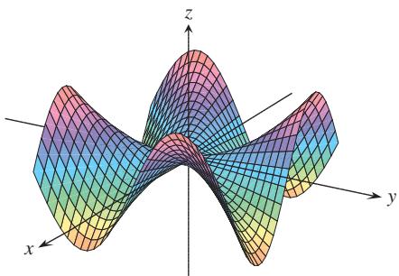
-
Finding a function from second partials Find a function
𝑤 = 𝑓 ( 𝑥 , 𝑦 ) 𝜕 𝑤 / 𝜕 𝑥 = 1 + 𝑒 𝑥 c o s 𝑦 𝜕 𝑤 / 𝜕 𝑦 = 2 𝑦 − 𝑒 𝑥 s i n 𝑦 -
A proof of Leibniz’s Rule Leibniz’s Rule says that if
𝑓 [ 𝑎 , 𝑏 ] 𝑢 ( 𝑥 ) 𝑣 ( 𝑥 ) 𝑥 [ 𝑎 , 𝑏 ]
Prove the rule by setting
and calculating dg/dx with the Chain Rule.
- Finding a function with constrained second partials Suppose that
𝑓 𝑟 𝑟 = √ 𝑥 2 + 𝑦 2 + 𝑧 2
Show that for some constants a and b,
- Homogeneous functions A function
𝑓 ( 𝑥 , 𝑦 ) 𝑓 ( 𝑡 𝑥 , 𝑡 𝑦 ) = 𝑡 𝑛 𝑓 ( 𝑥 , 𝑦 )
- Surface in polar coordinates Let
where r and
a.
b.
c.
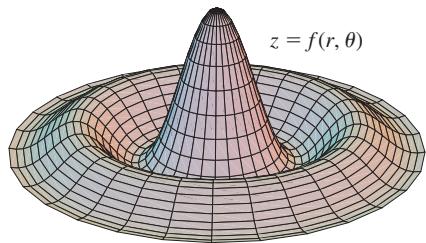
Gradients and Tangents
- Properties of position vectors Let
𝐫 = 𝑥 𝐢 + 𝑦 𝐣 + 𝑧 𝐤 𝑟 = | 𝐫 |
a. Show that
b. Show that
c. Find a function whose gradient equals r.
d. Show that
e. Show that
- Gradient orthogonal to tangent Suppose that a differentiable function
𝑓 ( 𝑥 , 𝑦 ) 𝑥 = 𝑔 ( 𝑡 ) 𝑦 = ℎ ( 𝑡 )
for all values of
- Curve tangent to a surface Show that the curve
is tangent to the surface
at
- Curve tangent to a surface Show that the curve
is tangent to the surface
at
Extreme Values
-
Extrema on a surface Show that the only possible maxima and minima of
𝑧 𝑧 = 𝑥 3 + 𝑦 3 − 9 𝑥 𝑦 + 2 7 𝑧 -
Maximum in closed first quadrant Find the maximum value of
𝑓 ( 𝑥 , 𝑦 ) = 6 𝑥 𝑦 𝑒 − ( 2 𝑥 + 3 𝑦 ) -
Minimum volume cut from first octant Find the minimum volume for a region bounded by the planes
𝑥 = 0 𝑦 = 0 𝑧 = 0
at a point in the first octant.
- Minimum distance from a line to a parabola in xy-plane By minimizing the function
𝑓 ( 𝑥 , 𝑦 , 𝑢 , 𝑣 ) = ( 𝑥 − 𝑢 ) 2 + ( 𝑦 − 𝑣 ) 2 𝑦 = 𝑥 + 1 𝑢 = 𝑣 2 𝑦 = 𝑥 + 1 𝑦 2 = 𝑥
Theory and Examples
-
Boundedness of first partials implies continuity Prove the following theorem: If
𝑓 ( 𝑥 , 𝑦 ) 𝑅 𝑥 𝑦 𝑓 𝑥 𝑓 𝑦 𝑅 𝑓 ( 𝑥 , 𝑦 ) 𝑅 -
Suppose that
𝐫 ( 𝑡 ) = 𝑔 ( 𝑡 ) 𝐢 + ℎ ( 𝑡 ) 𝐣 + 𝑘 ( 𝑡 ) 𝐤 𝑓 ( 𝑥 , 𝑦 , 𝑧 ) ∇ 𝑓 ∇ 𝑓 -
Finding functions from partial derivatives Suppose that
𝑓 𝑔 𝑥 𝑦
and suppose that
Find
-
Rate of change of the rate of change We know that if
𝑓 ( 𝑥 , 𝑦 ) 𝐮 = 𝑎 𝐢 + 𝑏 𝐣 𝐷 𝐮 𝑓 ( 𝑥 , 𝑦 ) = 𝑓 𝑥 ( 𝑥 , 𝑦 ) 𝑎 + 𝑓 𝑦 ( 𝑥 , 𝑦 ) 𝑏 𝑓 ( 𝑥 , 𝑦 ) ( 𝑥 , 𝑦 ) 𝐮 𝑓 ( 𝑥 , 𝑦 ) ( 𝑥 , 𝑦 ) 𝐮 -
Path of a heat-seeking particle A heat-seeking particle has the property that at any point
( 𝑥 , 𝑦 ) ( 𝑥 , 𝑦 ) 𝑇 ( 𝑥 , 𝑦 ) = − 𝑒 − 2 𝑦 c o s 𝑥 𝑦 = 𝑓 ( 𝑥 ) ( 𝜋 / 4 , 0 ) -
Velocity after a ricochet A particle traveling in a straight line with constant velocity
𝑖 + 𝑗 − 5 𝑘 ( 0 , 0 , 3 0 ) 𝑧 = 2 𝑥 2 + 3 𝑦 2 -
Directional derivatives tangent to a surface Let
𝑆 𝑓 ( 𝑥 , 𝑦 ) = 1 0 − 𝑥 2 − 𝑦 2 ( 𝑥 , 𝑦 , 𝑧 ) 𝑇 ( 𝑥 , 𝑦 , 𝑧 ) = 𝑥 2 𝑦 + 𝑦 2 𝑧 + 4 𝑥 + 1 4 𝑦 + 𝑧
a. Among all the possible directions tangential to the surface S at the point
b. Which direction tangential to S at the point
- Drilling another borehole On a flat surface of land, geologists drilled a borehole straight down and hit a mineral deposit at 300 m. They drilled a second borehole 30 m to the north of the first and hit the mineral deposit at 285 m. A third borehole 30 m east of the first borehole struck the mineral deposit at 307.5 m. The geologists have reasons to believe that the mineral deposit is in the shape of a dome, and for the sake of economy, they would like to find where the deposit is closest to the surface. Assuming the surface to be the xy-plane, in what direction from the first borehole would you suggest the geologists drill their fourth borehole?
The one-dimensional heat equation If
This equation is called the one-dimensional heat equation. The value of the positive constant
-
Find all solutions of the one-dimensional heat equation of the form
𝑤 = 𝑒 𝑟 𝑡 s i n 𝜋 𝑥 -
Find all solutions of the one-dimensional heat equation that have the form
𝑤 = 𝑒 𝑟 𝑡 s i n 𝑘 𝑥 𝑤 ( 0 , 𝑡 ) = 0 𝑤 ( 𝐿 , 𝑡 ) = 0 𝑡 → ∞
CHAPTER 13 Technology Application Projects
Mathematica/Maple Projects
Projects can be found within MyLab Math.
-
Plotting Surfaces Efficiently generate plots of surfaces, contours, and level curves.
-
Exploring the Mathematics Behind Skateboarding: Analysis of the Directional Derivative The path of a skateboarder is introduced, first on a level plane, then on a ramp, and finally on a paraboloid. Compute, plot, and analyze the directional derivative in terms of the skateboarder.
-
Looking for Patterns and Applying the Method of Least Squares to Real Data Fit a line to a set of numerical data points by choosing the line that minimizes the sum of the squares of the vertical distances from the points to the line.
-
Lagrange Goes Skateboarding: How High Does He Go? Revisit and analyze the skateboarders’ adventures for maximum and minimum heights from both a graphical and analytic perspective using Lagrange multipliers.