Chapter 3: Derivatives
3.1 Tangent Lines and the Derivative at a Point
In this section we define the slope and tangent line to a curve at a point, and the derivative of a function at a point. The derivative gives a way to find both the slope of a graph and the instantaneous rate of change of a function.
Finding a Tangent Line to the Graph of a Function
To find a tangent line to an arbitrary curve
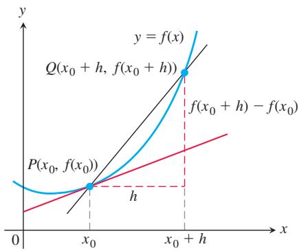
FIGURE 3.1 The slope of the tangent line at
DEFINITIONS The slope of the curve
at the point 𝑦 = 𝑓 ( 𝑥 ) is the number 𝑃 ( 𝑥 0 , 𝑓 ( 𝑥 0 ) ) l i m ℎ → 0 𝑓 ( 𝑥 0 + ℎ ) − 𝑓 ( 𝑥 0 ) ℎ (provided the limit exists).
The tangent line to the curve at P is the line through P with this slope.
In Section 2.1, Example 3, we applied these definitions to find the slope of the parabola
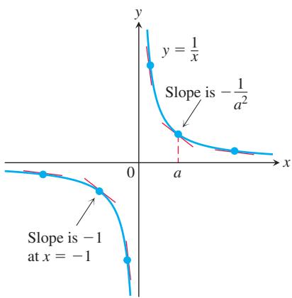
FIGURE 3.2 The tangent lines are steep when x is close to 0, and they become less steep as the point of tangency moves away (Example 1).
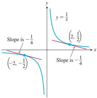
FIGURE 3.3 The two tangent lines to
The notation
EXAMPLE 1
(a) Find the slope of the curve
(b) Where does the slope equal
(c) What happens to the tangent line to the curve at the point
Solution
(a) Here
Notice how we had to keep writing “
(b) The slope of
This equation is equivalent to
(c) The slope
Rates of Change: Derivative at a Point
The expression
is called the difference quotient of f at
DEFINITION The derivative of a function
at a point 𝑓 , denoted 𝑥 0 , is 𝑓 ′ ( 𝑥 0 ) 𝑓 ′ ( 𝑥 0 ) = l i m ℎ → 0 𝑓 ( 𝑥 0 + ℎ ) − 𝑓 ( 𝑥 0 ) ℎ , provided this limit exists.
The derivative has more than one meaning, depending on what problem we are considering. The formula for the derivative is the same as the formula for the slope of the curve
EXAMPLE 2 In Examples 1 and 2 in Section 2.1, we studied the speed of a rock falling freely from rest near the surface of the earth. We knew that the rock fell
Solution We let
The rock’s speed at the instant
Our original estimate of 9.8 m/s in Section 2.1 was right.
Summary
We have been discussing slopes of curves, lines tangent to a curve, the rate of change of a function, and the derivative of a function at a point. All of these ideas are based on the same limit.
All of the following are interpretations for the limit of the difference quotient
-
The slope of the graph of
𝑦 = 𝑓 ( 𝑥 ) 𝑥 = 𝑥 0 -
The slope of the tangent line to the curve
𝑦 = 𝑓 ( 𝑥 ) 𝑥 = 𝑥 0 -
The rate of change of
𝑓 ( 𝑥 ) 𝑥 = 𝑥 0 -
The derivative
𝑓 ′ ( 𝑥 0 ) 𝑥 = 𝑥 0
In the next sections, we allow the point
EXERCISES 3.1
Slopes and Tangent Lines
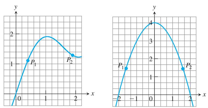
In Exercises 1–4, use the grid and a straight edge to make a rough estimate of the slope of the curve (in y-units per x-unit) at the points
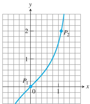
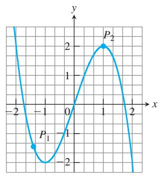
In Exercises 5–10, find an equation for the tangent line to the curve at the given point. Then sketch the curve and tangent line together.
-
𝑦 = 4 − 𝑥 2 , ( − 1 , 3 ) -
𝑦 = ( 𝑥 − 1 ) 2 + 1 , ( 1 , 1 ) -
𝑦 = 2 √ 𝑥 -
𝑦 = 1 𝑥 2 , ( − 1 , 1 ) -
𝑦 = 𝑥 3 , ( − 2 , − 8 ) -
𝑦 = 1 𝑥 3 , ( − 2 , − 1 8 )
In Exercises 11–18, find the slope of the function’s graph at the given point. Then find an equation for the line tangent to the graph there.
-
𝑓 ( 𝑥 ) = 𝑥 2 + 1 , ( 2 , 5 ) -
𝑓 ( 𝑥 ) = 𝑥 − 2 𝑥 2 , ( 1 , − 1 ) -
𝑔 ( 𝑥 ) = 𝑥 𝑥 − 2 , ( 3 , 3 ) -
𝑔 ( 𝑥 ) = 8 𝑥 2 , ( 2 , 2 ) -
ℎ ( 𝑡 ) = 𝑡 3 , ( 2 , 8 ) -
ℎ ( 𝑡 ) = 𝑡 3 + 3 𝑡 , -
𝑓 ( 𝑥 ) = √ 𝑥 , ( 4 , 2 ) -
𝑓 ( 𝑥 ) = √ 𝑥 + 1 , ( 8 , 3 )
In Exercises 19–22, find the slope of the curve at the point indicated.
-
𝑦 = 5 𝑥 − 3 𝑥 2 , 𝑥 = 1 -
𝑦 = 𝑥 3 − 2 𝑥 + 7 , 𝑥 = − 2 -
𝑦 = 1 𝑥 − 1 , 𝑥 = 3 -
𝑦 = 𝑥 − 1 𝑥 + 1 , 𝑥 = 0
Interpreting Derivative Values
- Growth of yeast cells In a controlled laboratory experiment, yeast cells are grown in an automated cell culture system that counts the number P of cells present at hourly intervals. The number after t hours is shown in the accompanying figure.
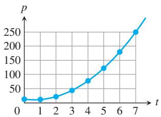
a. Explain what is meant by the derivative
b. Which is larger,
c. The quadratic curve capturing the trend of the data points (see Appendix A.2) is given by
- Effectiveness of a drug On a scale from 0 to 1, the effectiveness E of a pain-killing drug t hours after entering the bloodstream is displayed in the accompanying figure.
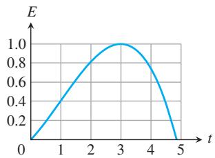
a. At what times does the effectiveness appear to be increasing? What is true about the derivative at those times?
b. At what time would you estimate that the drug reaches its maximum effectiveness? What is true about the derivative at that time? What is true about the derivative as time increases in the 1 hour before your estimated time?
At what points do the graphs of the functions in Exercises 25 and 26 have horizontal tangent lines?
-
𝑓 ( 𝑥 ) = 𝑥 2 + 4 𝑥 − 1 2 6 . 𝑔 ( 𝑥 ) = 𝑥 3 − 3 𝑥 -
Find equations of all lines having slope -1 that are tangent to the curve
𝑦 = 1 / ( 𝑥 − 1 ) -
Find an equation of the straight line having slope 1/4 that is tangent to the curve
𝑦 = √ 𝑥
Rates of Change
-
Object dropped from a tower An object is dropped from the top of a 100-m-high tower. Its height above ground after
𝑡 1 0 0 − 4 . 9 𝑡 2 -
Speed of a rocket At t seconds after liftoff, the height of a rocket is
3 𝑡 2 -
Disk’s changing area What is the rate of change of the area of a disk
( 𝐴 = 𝜋 𝑟 2 ) 𝑟 = 3 -
Ball’s changing volume What is the rate of change of the volume of a ball
( 𝑉 = ( 4 / 3 ) 𝜋 𝑟 3 ) 𝑟 = 2 -
Show that the line
𝑦 = 𝑚 𝑥 + 𝑏 ( 𝑥 0 , 𝑚 𝑥 0 + 𝑏 ) -
Find the slope of the tangent line to the curve
𝑦 = 1 / √ 𝑥
Testing for Tangent Lines
- Does the graph of
have a tangent line at the origin? Give reasons for your answer.
- Does the graph of
have a tangent line at the origin? Give reasons for your answer.
Vertical Tangent Lines
We say that a continuous curve
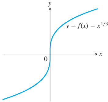
VERTICAL TANGENT LINE AT ORIGIN
However,
does not exist, because the limit is
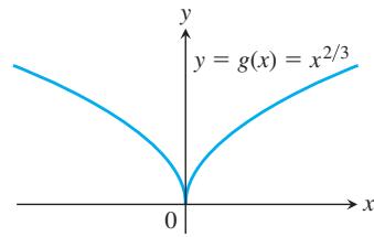
NO VERTICAL TANGENT LINE AT ORIGIN
- Does the graph of
have a vertical tangent line at the origin? Give reasons for your answer.
- Does the graph of
have a vertical tangent line at the point
T Graph the curves in Exercises 39–48.
a. Where do the graphs appear to have vertical tangent lines?
b. Confirm your findings in part (a) with limit calculations. But before you do, read the introduction to Exercises 37 and 38.
-
𝑦 = 𝑥 2 / 5 -
𝑦 = 𝑥 4 / 5 -
𝑦 = 𝑥 1 / 5 -
𝑦 = 𝑥 3 / 5 -
𝑦 = 4 𝑥 2 / 5 − 2 𝑥 -
𝑦 = 𝑥 5 / 3 − 5 𝑥 2 / 3 -
𝑦 = 𝑥 2 / 3 − ( 𝑥 − 1 ) 1 / 3 -
𝑦 = 𝑥 1 / 3 + ( 𝑥 − 1 ) 1 / 3 -
𝑦 = { − √ | 𝑥 | , 𝑥 ≤ 0 √ 𝑥 , 𝑥 > 0 -
𝑦 = √ | 4 − 𝑥 |
COMPUTER EXPLORATIONS
Use a CAS to perform the following steps for the functions in Exercises 49–52:
a. Plot
b. Holding
at
c. Find the limit of q as
d. Define the secant lines
-
𝑓 ( 𝑥 ) = 𝑥 + 5 𝑥 , 𝑥 0 = 1 -
𝑓 ( 𝑥 ) = 𝑥 + s i n ( 2 𝑥 ) 𝑥 0 = 𝜋 / 2 -
𝑓 ( 𝑥 ) = c o s 𝑥 + 4 s i n ( 2 𝑥 ) 𝑥 0 = 𝜋
3.2 The Derivative as a Function
HISTORICAL ESSAY
In the last section we defined the derivative of
The Derivative
To read this essay, visit the companion Website.
We now investigate the derivative as a function derived from f by considering the limit at each point x in the domain of f.
DEFINITION The derivative of the function
with respect to the variable 𝑓 ( 𝑥 ) is the function 𝑥 whose value at 𝑓 ′ is 𝑥 𝑓 ′ ( 𝑥 ) = l i m ℎ → 0 𝑓 ( 𝑥 + ℎ ) − 𝑓 ( 𝑥 ) ℎ , provided the limit exists.
We use the notation
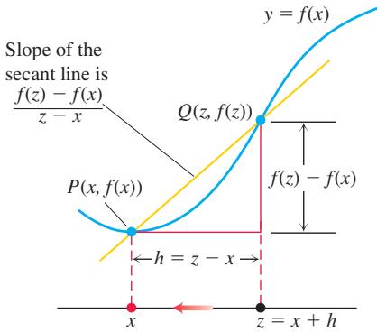
FIGURE 3.4 Two forms for the difference quotient.
Derivative of the Reciprocal Function
which the limit exists, which means that the domain may be the same as or smaller than the domain of f. If
If we write
Alternative Formula for the Derivative
Calculating Derivatives from the Definition
The process of calculating a derivative is called differentiation. To emphasize the idea that differentiation is an operation performed on a function
as another way to denote the derivative
Here are two more examples in which we allow x to be any point in the domain of f.
EXAMPLE 1 Differentiate
Solution We use the definition of derivative, which requires us to calculate
EXAMPLE 2
(a) Find the derivative of
(b) Find the tangent line to the curve
Derivative of the Square Root Function
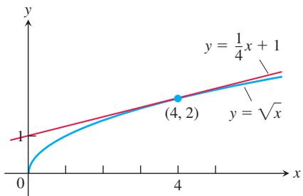
FIGURE 3.5 The curve
(a)
(b)
FIGURE 3.6 We made the graph of
Solution
(a) We use the alternative formula to calculate
(b) The slope of the curve at
The tangent line is the line through the point
Notation
There are many ways to denote the derivative of a function
The symbols d/dx and D indicate the operation of differentiation. We read dy/dx as “the derivative of y with respect to x,” and df/dx and
To indicate the value of a derivative at a specified number x = a, we use the notation
For instance, in Example 2,
Graphing the Derivative
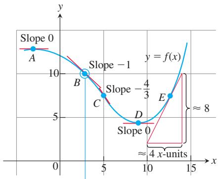
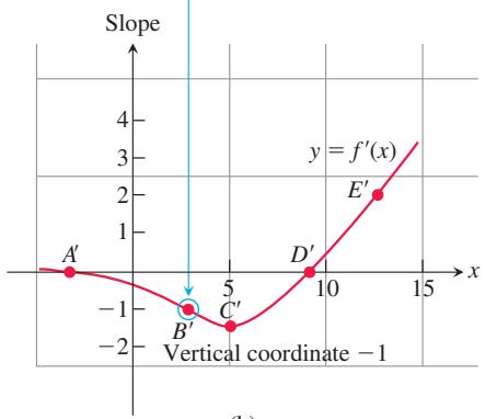
We can often make an approximate plot of the derivative of
EXAMPLE 3 Graph the derivative of the function
Solution We sketch the tangent lines to the graph of f at frequent intervals and use their slopes to estimate the values of
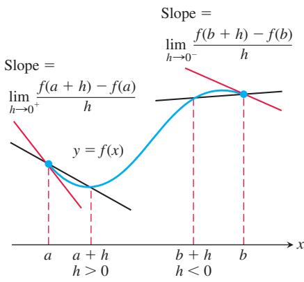
FIGURE 3.7 Derivatives at endpoints of a closed interval are one-sided limits.
What can we learn from the graph of
FIGURE 3.8 The function
-
where the rate of change of
𝑓 -
the rough size of the growth rate at any x;
-
where the rate of change itself is increasing or decreasing.
Differentiability on an Interval; One-Sided Derivatives
A function
exist at the endpoints (Figure 3.7).
Right-hand and left-hand derivatives may or may not be defined at any point of a function’s domain. Because of Theorem 5, Section 2.4, a function has a derivative at an interior point if and only if it has left-hand and right-hand derivatives there, and these one-sided derivatives are equal.
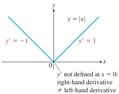
EXAMPLE 4 Show that the function
Solution The graph of the function
To the left, when x < 0,
(Figure 3.8). The two branches of the graph come together at an angle at the origin, forming a non-smooth corner. There is no derivative at the origin because the one-sided derivatives differ there:
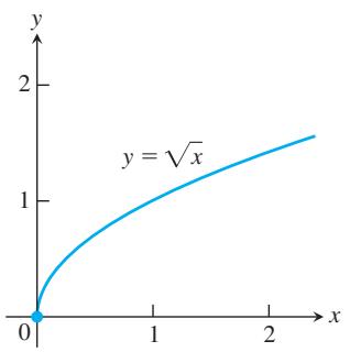
FIGURE 3.9 The square root function is not differentiable at x = 0, where the graph of the function has a vertical tangent line.
EXAMPLE 5 In Example 2 we found that for x > 0,
We apply the definition to examine whether the derivative exists at x = 0:
Since the (right-hand) limit is not finite, there is no derivative at x = 0. Since the slopes of the secant lines joining the origin to the points
When Does a Function Not Have a Derivative at a Point?
A function has a derivative at a point
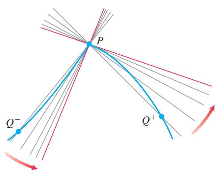
- a corner, where the one-sided derivatives differ
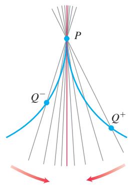
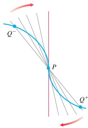
-
a cusp, where the slope of PQ approaches
∞ − ∞ -
a vertical tangent line, where the slope of PQ approaches
∞ − ∞ − ∞
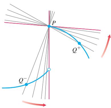
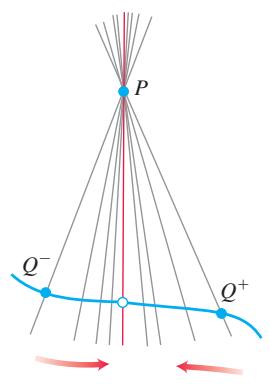
- a discontinuity (two examples shown)
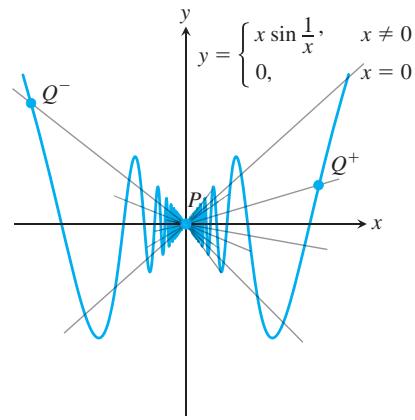
- wild oscillation
The last example shows a function that is continuous at x = 0, but whose graph oscillates wildly up and down as it approaches x = 0. The slopes of the secant lines through 0 oscillate between -1 and 1 as x approaches 0, and do not have a limit at x = 0.
Differentiable Functions Are Continuous
A function is continuous at every point where it has a derivative.
THEOREM 1—Differentiable Implies Continuous If
Proof Given that
Now take limits as
Similar arguments with one-sided limits show that if
Theorem 1 says that if a function has a discontinuity at a point (for instance, a jump discontinuity), then it cannot be differentiable there. The greatest integer function
Caution The converse of Theorem 1 is false. A function need not have a derivative at a point where it is continuous, as we saw with the absolute value function in Example 4.
EXERCISES 3.2
Finding Derivative Functions and Values
Using the definition, calculate the derivatives of the functions in Exercises 1–6. Then find the values of the derivatives as specified.
In Exercises 7–12, find the indicated derivatives.
-
𝑑 𝑦 𝑑 𝑥 𝑦 = 2 𝑥 3 -
𝑑 𝑟 𝑑 𝑠 i f 𝑟 = 𝑠 3 − 2 𝑠 2 + 3 -
𝑑 𝑠 𝑑 𝑡 𝑠 = 𝑡 2 𝑡 + 1 -
𝑑 𝑣 𝑑 𝑡 𝑣 = 𝑡 − 1 𝑡 -
𝑑 𝑝 𝑑 𝑞 𝑝 = 𝑞 3 / 2 -
𝑑 𝑧 𝑑 𝑤 𝑧 = 1 √ 𝑤 2 − 1
Slopes and Tangent Lines
In Exercises 13–16, differentiate the functions and find the slope of the tangent line at the given value of the independent variable.
-
𝑓 ( 𝑥 ) = 𝑥 + 9 𝑥 , 𝑥 = − 3 -
𝑘 ( 𝑥 ) = 1 2 + 𝑥 , 𝑥 = 2 -
𝑠 = 𝑡 3 − 𝑡 2 , 𝑡 = − 1 -
𝑦 = 𝑥 + 3 1 − 𝑥 , 𝑥 = − 2
In Exercises 17–18, differentiate the functions. Then find an equation of the tangent line at the indicated point on the graph of the function.
-
𝑦 = 𝑓 ( 𝑥 ) = 8 √ 𝑥 − 2 , ( 𝑥 , 𝑦 ) = ( 6 , 4 ) -
𝑤 = 𝑔 ( 𝑧 ) = 1 + √ 4 − 𝑧 , ( 𝑧 , 𝑤 ) = ( 3 , 2 )
In Exercises 19–22, find the values of the derivatives.
-
𝑑 𝑠 𝑑 𝑡 ∣ 𝑡 = − 1 i f 𝑠 = 1 − 3 𝑡 2 -
𝑑 𝑦 𝑑 𝑥 ∣ 𝑥 = √ 3 i f 𝑦 = 1 − 1 𝑥 -
𝑑 𝑟 𝑑 𝜃 ∣ 𝜃 = 0 𝑟 = 2 √ 4 − 𝜃 -
𝑑 𝑤 𝑑 𝑧 ∣ 𝑧 = 4 𝑤 = 𝑧 + √ 𝑧
Using the Alternative Formula for Derivatives Use the formula
to find the derivative of the functions in Exercises 23-26.
-
𝑓 ( 𝑥 ) = 1 𝑥 + 2 -
𝑓 ( 𝑥 ) = 𝑥 2 − 3 𝑥 + 4 -
𝑔 ( 𝑥 ) = 𝑥 𝑥 − 1 -
𝑔 ( 𝑥 ) = 1 + √ 𝑥
Graphs
Match the functions graphed in Exercises 27–30 with the derivatives graphed in the accompanying figures (a)–(d).
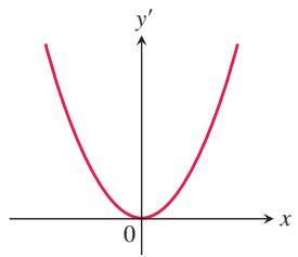
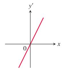
(a)
(b)
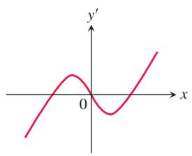
(c)
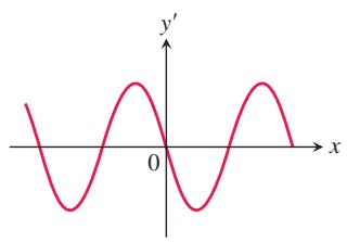
(d)
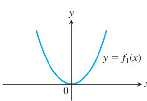
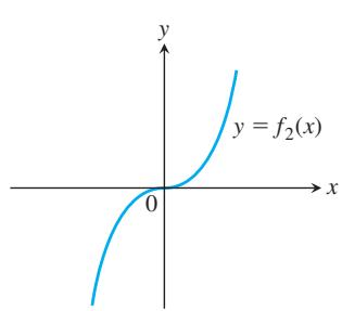
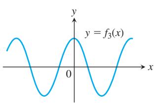
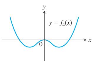
- Consider the function
𝑓 𝑓 [ − 4 , 6 ]
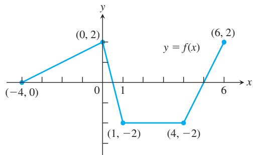
a. At which points of the domain interval is
b. Graph the derivative of
- Recovering a function from its derivative
a. Use the following information to graph the function
i) The graph of
ii) The graph starts at the point
iii) The derivative of
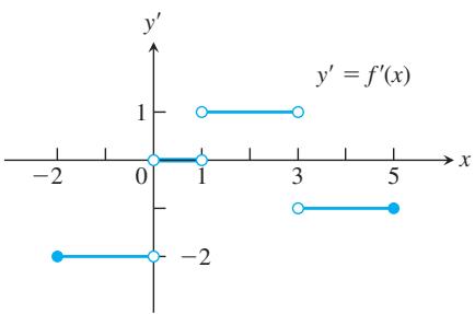
b. Repeat part (a), assuming that the graph starts at
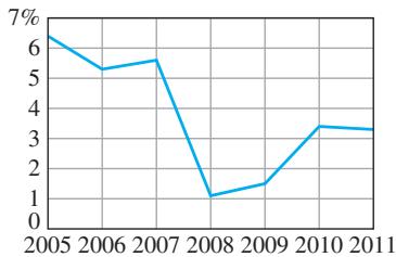
- Growth in the economy The graph in the accompanying figure shows the average annual percentage change
𝑦 = 𝑓 ( 𝑡 )
- Fruit flies (Continuation of Example 4, Section 2.1.) Populations starting out in closed environments grow slowly at first, when there are relatively few members, then more rapidly as the number of reproducing individuals increases and resources are still abundant, then slowly again as the population reaches the carrying capacity of the environment.
a. Use the graphical technique of Example 3 to graph the derivative of the fruit fly population as a function of time (in days). The graph of the population is reproduced here.
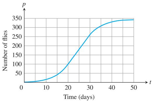
b. During what days does the population seem to be increasing fastest? Slowest?
- Temperature The given graph shows the temperature
𝑇 ∘ C
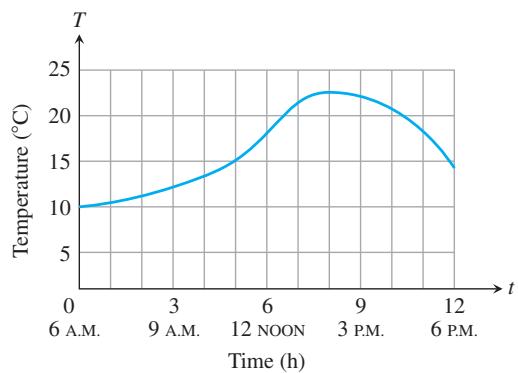
a. Estimate the rate of temperature change at the times i) 7 A.M. ii) 9 A.M. iii) 2 P.M. iv) 4 P.M.
b. At what time does the temperature increase most rapidly? Decrease most rapidly? What is the rate for each of those times?
c. Use the graphical technique of Example 3 to graph the derivative of temperature T versus time t.
- Average single-family home prices P (in thousands of dollars) in Sacramento, California, are shown in the accompanying figure from the beginning of 2006 through the end of 2015.
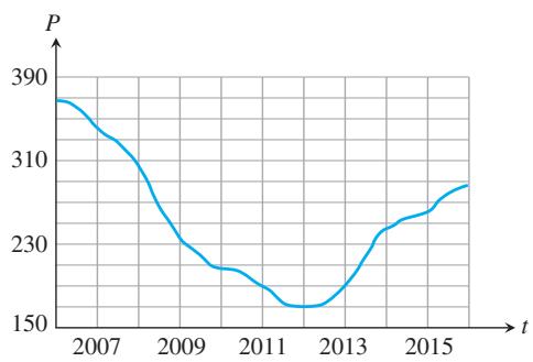
a. During what years did home prices decrease? increase? b. Estimate home prices at the end of i) 2007 ii) 2012 iii) 2015
c. Estimate the rate of change of home prices at the beginning of i) 2007 ii) 2010 iii) 2014
d. During what year did home prices drop most rapidly and what is an estimate of this rate?
e. During what year did home prices rise most rapidly and what is an estimate of this rate?
f. Use the graphical technique of Example 3 to graph the derivative of home price P versus time t.
One-Sided Derivatives
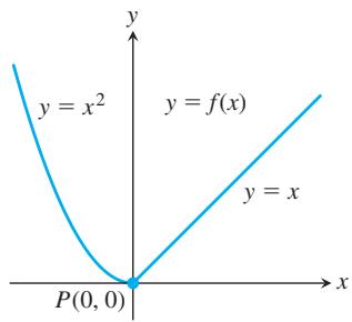
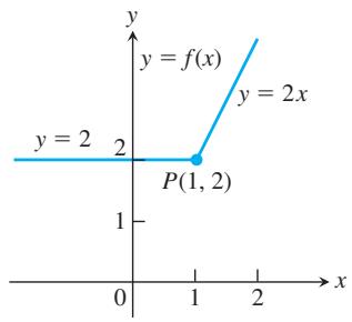
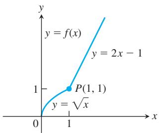
Compute the right-hand and left-hand derivatives as limits to show that the functions in Exercises 37–40 are not differentiable at the point P. 37. 38.
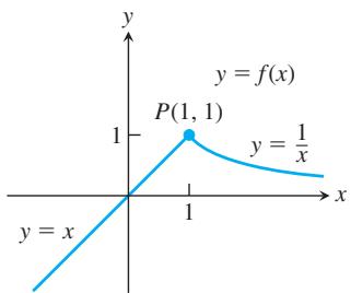
In Exercises 41–44, determine whether the piecewise-defined function is differentiable at x = 0.
-
𝑓 ( 𝑥 ) = { 2 𝑥 − 1 , 𝑥 ≥ 0 𝑥 2 + 2 𝑥 + 7 , 𝑥 < 0 -
𝑔 ( 𝑥 ) = { 𝑥 2 / 3 , 𝑥 ≥ 0 𝑥 1 / 3 , 𝑥 < 0 -
𝑓 ( 𝑥 ) = { 2 𝑥 + t a n 𝑥 , 𝑥 ≥ 0 𝑥 2 , 𝑥 < 0 -
𝑔 ( 𝑥 ) = { 2 𝑥 − 𝑥 3 − 1 , 𝑥 ≥ 0 𝑥 − 1 𝑥 + 1 , 𝑥 < 0
Differentiability and Continuity on an Interval
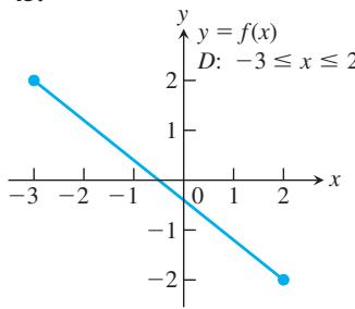
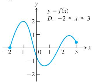
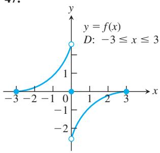
Each figure in Exercises 45–50 shows the graph of a function over a closed interval D. At what domain points does the function appear to be
a. differentiable?
b. continuous but not differentiable?
c. neither continuous nor differentiable?
Give reasons for your answers.
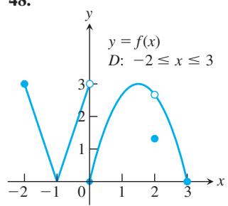
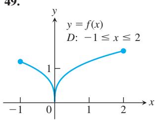
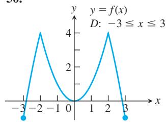
Theory and Examples
In Exercises 51–54,
a. Find the derivative
b. Graph
c. For what values of
d. Over what intervals of
-
𝑦 = − 𝑥 2 -
𝑦 = − 1 / 𝑥 -
𝑦 = 𝑥 3 / 3 -
𝑦 = 𝑥 4 / 4 -
Tangent line to a parabola Does the parabola
𝑦 = 2 𝑥 2 − 1 3 𝑥 + 5 -
Tangent line to
𝑦 = √ 𝑥 𝑦 = √ 𝑥 -
Derivative of
− 𝑓 𝑓 ( 𝑥 ) 𝑥 = 𝑥 0 − 𝑓 𝑥 = 𝑥 0 -
Derivative of multiples Does knowing that a function
𝑔 ( 𝑡 ) -
Limit of a quotient Suppose that functions
𝑔 ( 𝑡 ) ℎ ( 𝑡 ) 𝑡 𝑔 ( 0 ) = ℎ ( 0 ) = 0 l i m 𝑡 → 0 𝑔 ( 𝑡 ) / ℎ ( 𝑡 ) -
a. Let
𝑓 ( 𝑥 ) | 𝑓 ( 𝑥 ) | ≤ 𝑥 2 − 1 ≤ 𝑥 ≤ 1 𝑓 𝑥 = 0 𝑓 ′ ( 0 )
b. Show that
is differentiable at
T 61. Graph
for
- Graph
𝑦 = 3 𝑥 2 − 2 ≤ 𝑥 ≤ 2 , 0 ≤ 𝑦 ≤ 3
for
-
Derivative of
𝑦 = | 𝑥 | 𝑓 ( 𝑥 ) = | 𝑥 | 𝑦 = ( | 𝑥 | − 0 ) / ( 𝑥 − 0 ) = | 𝑥 | / 𝑥 -
Weierstrass’s nowhere differentiable continuous function The sum of the first eight terms of the Weierstrass function
𝑓 ( 𝑥 ) = ∑ ∞ 𝑛 = 0 ( 2 / 3 ) 𝑛 c o s ( 9 𝑛 𝜋 𝑥 )
Graph this sum. Zoom in several times. How wiggly and bumpy is this graph? Specify a viewing window in which the displayed portion of the graph is smooth.
COMPUTER EXPLORATIONS
Use a CAS to perform the following steps for the functions in Exercises 65–70.
a. Plot
b. Define the difference quotient q at a general point x, with general step size h.
c. Take the limit as
d. Substitute the value
e. Substitute various values for
f. Graph the formula obtained in part (c). What does it mean when its values are negative? Zero? Positive? Does this make sense with your plot from part (a)? Give reasons for your answer.
-
𝑓 ( 𝑥 ) = 𝑥 3 + 𝑥 2 − 𝑥 , 𝑥 0 = 1 -
𝑓 ( 𝑥 ) = 𝑥 1 / 3 + 𝑥 2 / 3 , 𝑥 0 = 1
𝑓 ( 𝑥 ) = 4 𝑥 𝑥 2 + 1 , 𝑥 0 = 2
3.3 Differentiation Rules
This section introduces several rules that allow us to differentiate constant functions, power functions, polynomials, exponential functions, rational functions, and certain combinations of them, simply and directly, without having to take limits each time.
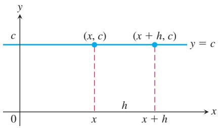
A basic rule of differentiation is that the derivative of every constant function is zero.
Powers, Multiples, Sums, and Differences
FIGURE 3.10 The rule
Derivative of a Constant Function
If
To know more, visit the companion Website.
Proof We apply the definition of the derivative to
We now consider powers of
From Example 2 of the last section we also know that
These two examples illustrate a general rule for differentiating a power
Derivative of a Positive Integer Power
If
HISTORICAL BIOGRAPHY
Courant obtained a PhD from Göttingen in 1910. He founded Göttingen’s Mathematics Institute and was its director from 1920 until 1933. His research work focused on mathematical physics.
Richard Courant (1888–1972)
Proof of the Positive Integer Power Rule The formula
can be verified by multiplying out the right-hand side. Then, from the alternative formula for the definition of the derivative,
The Power Rule is actually valid for all real numbers n, not just for positive integers. We have seen examples for a negative integer and fractional power, but n could be an irrational number as well. Here we state the general version of the rule, but postpone its proof until Section 3.8.
Power Rule (General Version)
If
for all
EXAMPLE 1 Differentiate the following powers of x.
(a)
Applying the Power Rule
Solution
Subtract 1 from the exponent and multiply the result by the original exponent.
(a)
The next rule says that when a differentiable function is multiplied by a constant, its derivative is multiplied by the same constant.
Derivative Constant Multiple Rule
If u is a differentiable function of x, and c is a constant, then
Proof
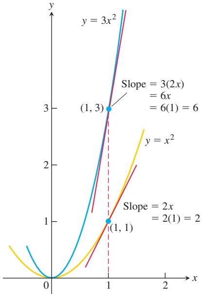
FIGURE 3.11 The graphs of
Denoting Functions by 𝑢 𝜐
The functions we are working with when we need a differentiation formula are likely to be denoted by letters like f and g. We do not want to use these same letters when stating general differentiation rules, so instead we use letters like u and v that are not likely to be already in use.
EXAMPLE 2
(a) The derivative formula
says that if we rescale the graph of
(b) Negative of a function
The derivative of the negative of a differentiable function
The next rule says that the derivative of the sum of two differentiable functions is the sum of their derivatives.
Derivative Sum Rule
If u and v are differentiable functions of x, then their sum
Proof We apply the definition of the derivative to
Combining the Sum Rule with the Constant Multiple Rule gives the Difference Rule, which says that the derivative of a difference of differentiable functions is the difference of their derivatives:
The Sum Rule also extends to finite sums of more than two functions. If
A proof by mathematical induction for any finite number of terms is given in Appendix A.3.
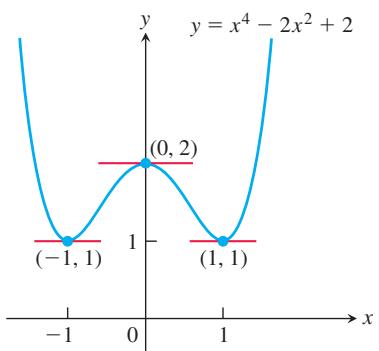
FIGURE 3.12 The curve in Example 4 and its horizontal tangent lines.
EXAMPLE 3 Find the derivative of the polynomial
Solution
We can differentiate any polynomial term by term, the way we differentiated the polynomial in Example 3. All polynomials are differentiable at all values of x.
EXAMPLE 4 Does the curve
Solution The horizontal tangent lines, if any, occur where the slope dy/dx is zero. We have
Now solve the equation
The curve
Derivatives of Exponential Functions
We briefly reviewed exponential functions in Section 1.4. When we apply the definition of the derivative to
Thus we see that the derivative of
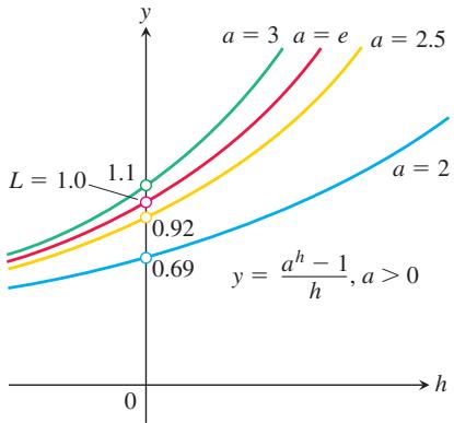
FIGURE 3.13 The position of the curve
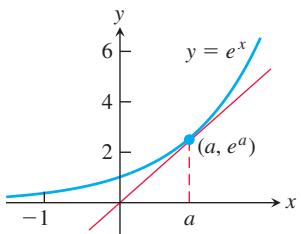
FIGURE 3.14 The line through the origin is tangent to the graph of
The limit L is therefore the slope of the graph of
Figure 3.13 shows the graphs of
because it is the exponential function whose graph has slope 1 when it crosses the y-axis. That the limit is 1 implies an important relationship between the natural exponential function
Therefore the natural exponential function is its own derivative.
Derivative of the Natural Exponential Function
EXAMPLE 5 Find an equation for a line that is tangent to the graph of
Solution Since the line passes through the origin, its equation is of the form y = mx, where m is the slope. If it is tangent to the graph at the point
We might ask if there are functions other than the natural exponential function that are their own derivatives. The answer is that the only functions that satisfy the property that
Products and Quotients
While the derivative of the sum of two functions is the sum of their derivatives, the derivative of the product of two functions is not the product of their derivatives. For instance,
The derivative of a product of two functions is the sum of two products, as we now explain.
Derivative Product Rule
If u and v are differentiable at x, then so is their product uv, and
The derivative of the product uv is u times the derivative of v plus the derivative of u times v. In prime notation,
EXAMPLE 6 Find the derivative of (a)
Solution
(a) We apply the Product Rule with
Picturing the Product Rule
Suppose
Division by
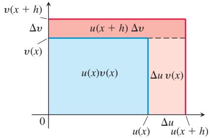
Then the change in the product uv is the difference in areas of the larger and smaller “boxes,” which is the sum of the areas of the upper and right-hand reddish-shaded rectangles. That is,
The limit as
Proof of the Derivative Product Rule
To change this fraction into an equivalent one that contains difference quotients for the derivatives of u and v, we subtract and add
As h approaches zero,
The derivative of the quotient of two functions is given by the Quotient Rule.
Derivative Quotient Rule
If u and v are differentiable at x and if
In function notation,
EXAMPLE 7 Find the derivative of (a)
Solution
(a) We apply the Quotient Rule with
Proof of the Derivative Quotient Rule
To change the last fraction into an equivalent one that contains the difference quotients for the derivatives of
Taking the limits in the numerator and denominator now gives the Quotient Rule. Exercise 76 outlines another proof.
The choice of which rules to use in solving a differentiation problem can make a difference in how much work you have to do. Here is an example.
EXAMPLE 8 Find the derivative of
HISTORICAL BIOGRAPHY
Maria Gaetana Agnesi (1718–1799)
Agnesi was a well-published scientist by age 20 and an honorary faculty member of the University of Bologna by age 30. Today, Agnesi is remembered chiefly for a bell-shaped curve called the “Witch of Agnesi.”
To know more, visit the companion Website.
How to Read the Symbols for Derivatives
y’ “y prime”
y” “y double prime”
y''' “y triple prime”
Solution Using the Quotient Rule here will result in a complicated expression with many terms. Instead, use some algebra to simplify the expression. First expand the numerator and divide by
Then use the Sum, Constant Multiple, and Power Rules:
Second- and Higher-Order Derivatives
If
The symbol
If
Thus
If
denoting the nth derivative of y with respect to x for any positive integer n.
We can interpret the second derivative as the rate of change of the slope of the tangent line to the graph of
EXAMPLE 9 The first four derivatives of
First derivative:
Second derivative:
Third derivative:
Fourth derivative:
All polynomial functions have derivatives of all orders. In this example, the fifth and later derivatives are all zero.
Exercises 3.3
Derivative Calculations
In Exercises 1–12, find the first and second derivatives.
-
𝑦 = − 𝑥 2 + 3 -
𝑦 = 𝑥 2 + 𝑥 + 8 -
𝑠 = 5 𝑡 3 − 3 𝑡 5 -
𝑤 = 3 𝑧 7 − 7 𝑧 3 + 2 1 𝑧 2 -
𝑦 = 4 𝑥 3 3 − 𝑥 + 2 𝑒 𝑥 -
𝑦 = 𝑥 3 3 + 𝑥 2 2 + 𝑒 − 𝑥 -
𝑤 = 3 𝑧 − 2 − 1 𝑧 -
𝑠 = − 2 𝑡 − 1 + 4 𝑡 2 -
𝑦 = 6 𝑥 2 − 1 0 𝑥 − 5 𝑥 − 2 -
𝑦 = 4 − 2 𝑥 − 𝑥 − 3 -
𝑟 = 1 3 𝑠 2 − 5 2 𝑠 -
𝑟 = 1 2 𝜃 − 4 𝜃 3 + 1 𝜃 4
In Exercises 13–16, find
-
𝑦 = ( 3 − 𝑥 2 ) ( 𝑥 3 − 𝑥 + 1 ) -
𝑦 = ( 2 𝑥 + 3 ) ( 5 𝑥 2 − 4 𝑥 ) -
𝑦 = ( 𝑥 2 + 1 ) ( 𝑥 + 5 + 1 𝑥 ) -
𝑦 = ( 1 + 𝑥 2 ) ( 𝑥 3 / 4 − 𝑥 − 3 )
Find the derivatives of the functions in Exercises 17–40.
-
𝑦 = 2 𝑥 + 5 3 𝑥 − 2 -
𝑧 = 4 − 3 𝑥 3 𝑥 2 + 𝑥 -
𝑔 ( 𝑥 ) = 𝑥 2 − 4 𝑥 + 0 . 5 -
𝑓 ( 𝑡 ) = 𝑡 2 − 1 𝑡 2 + 𝑡 − 2 -
𝑣 = ( 1 − 𝑡 ) ( 1 + 𝑡 2 ) − 1 -
𝑤 = ( 2 𝑥 − 7 ) − 1 ( 𝑥 + 5 ) -
𝑓 ( 𝑠 ) = √ 𝑠 − 1 √ 𝑠 + 1 -
𝑢 = 5 𝑥 + 1 2 √ 𝑥 -
𝑣 = 1 + 𝑥 − 4 √ 𝑥 𝑥 -
𝑟 = 2 ( 1 √ 𝜃 + √ 𝜃 ) -
𝑦 = 1 ( 𝑥 2 − 1 ) ( 𝑥 2 + 𝑥 + 1 ) -
𝑦 = ( 𝑥 + 1 ) ( 𝑥 + 2 ) ( 𝑥 − 1 ) ( 𝑥 − 2 ) -
𝑦 = 2 𝑒 − 𝑥 + 𝑒 3 𝑥 -
𝑦 = 𝑥 2 + 3 𝑒 𝑥 2 𝑒 𝑥 − 𝑥 -
𝑦 = 𝑥 3 𝑒 𝑥 -
𝑤 = 𝑟 𝑒 − 𝑟 -
𝑦 = 𝑥 9 / 4 + 𝑒 − 2 𝑥 -
𝑦 = 𝑥 − 3 / 5 + 𝜋 3 / 2 -
𝑠 = 2 𝑡 3 / 2 + 3 𝑒 2 -
𝑤 = 1 𝑧 1 . 4 + 𝜋 √ 𝑧 -
𝑦 = 7 √ 𝑥 2 − 𝑥 𝑒 -
𝑦 = 3 √ 𝑥 9 . 6 + 2 𝑒 1 . 3 -
𝑟 = 𝑒 𝑠 𝑠 -
𝑟 = 𝑒 𝜃 ( 1 𝜃 2 + 𝜃 − 𝜋 / 2 )
Find the derivatives of all orders of the functions in Exercises 41-44.
-
𝑦 = 𝑥 4 2 − 3 2 𝑥 2 − 𝑥 -
𝑦 = 𝑥 5 1 2 0 -
𝑦 = ( 𝑥 − 1 ) ( 𝑥 + 2 ) ( 𝑥 + 3 ) -
𝑦 = ( 4 𝑥 2 + 3 ) ( 2 − 𝑥 ) 𝑥
Find the first and second derivatives of the functions in Exercises 45–52.
-
𝑦 = 𝑥 3 + 7 𝑥 -
𝑠 = 𝑡 2 + 5 𝑡 − 1 𝑡 2 -
𝑟 = ( 𝜃 − 1 ) ( 𝜃 2 + 𝜃 + 1 ) 𝜃 3 -
𝑢 = ( 𝑥 2 + 𝑥 ) ( 𝑥 2 − 𝑥 + 1 ) 𝑥 4 -
𝑤 = ( 1 + 3 𝑧 3 𝑧 ) ( 3 − 𝑧 ) -
𝑝 = 𝑞 2 + 3 ( 𝑞 − 1 ) 3 + ( 𝑞 + 1 ) 3 -
𝑤 = 3 𝑧 2 𝑒 2 𝑧 -
𝑤 = 𝑒 𝑧 ( 𝑧 − 1 ) ( 𝑧 2 + 1 ) -
Suppose
𝑢 𝑣 𝑥 𝑥 = 0
Find the values of the following derivatives at
a.
- Suppose u and v are differentiable functions of x and that
Find the values of the following derivatives at x = 1.
a.
Slopes and Tangent Lines
- a. Normal line to a curve Find an equation for the line perpendicular to the tangent line to the curve
𝑦 = 𝑥 3 − 4 𝑥 + 1
b. Smallest slope What is the smallest slope on the curve? At what point on the curve does the curve have this slope?
c. Tangent lines having specified slope Find equations for the tangent lines to the curve at the points where the slope of the curve is 8.
- a. Horizontal tangent lines Find equations for the horizontal tangent lines to the curve
𝑦 = 𝑥 3 − 3 𝑥 − 2
b. Smallest slope What is the smallest slope on the curve? At what point on the curve does the curve have this slope? Find an equation for the line that is perpendicular to the curve’s tangent line at this point.
- Find the tangent lines to Newton’s serpentine (graphed here) at the origin and the point
( 1 , 2 )
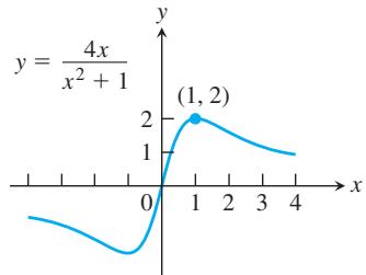
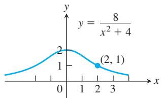
- Find the tangent line to the Witch of Agnesi (graphed here) at the point
( 2 , 1 )
-
Quadratic tangent to identity function The curve
𝑦 = 𝑎 𝑥 2 + 𝑏 𝑥 + 𝑐 -
Quadratics having a common tangent line The curves
𝑦 = 𝑥 2 + 𝑎 𝑥 + 𝑏 𝑦 = 𝑐 𝑥 − 𝑥 2 𝑎 , 𝑏 , 𝑐 -
Find all points
( 𝑥 , 𝑦 ) 𝑓 ( 𝑥 ) = 3 𝑥 2 − 4 𝑥 𝑦 = 8 𝑥 + 5 -
Find all points
( 𝑥 , 𝑦 ) 𝑔 ( 𝑥 ) = 1 3 𝑥 3 − 3 2 𝑥 2 + 1 -
Find all points
( 𝑥 , 𝑦 ) 𝑦 = 𝑥 / ( 𝑥 − 2 ) 𝑦 = 2 𝑥 + 3 -
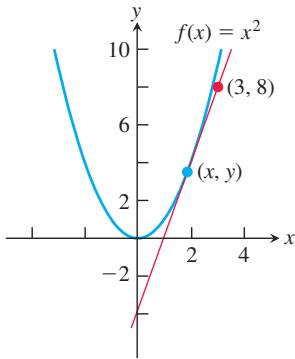
Find all points
( 𝑥 , 𝑦 ) 𝑓 ( 𝑥 ) = 𝑥 2 ( 3 , 8 )
-
Assume that functions f and g are differentiable with
𝑓 ( 1 ) = 2 𝑓 ′ ( 1 ) = − 3 𝑔 ( 1 ) = 4 𝑔 ′ ( 1 ) = − 2 𝐹 ( 𝑥 ) = 𝑓 ( 𝑥 ) 𝑔 ( 𝑥 ) -
Assume that functions
𝑓 𝑔 𝑓 ( 2 ) = 3 𝑓 ′ ( 2 ) = − 1 𝑔 ( 2 ) = − 4 𝑔 ′ ( 2 ) = 1 𝐹 ( 𝑥 ) = 𝑓 ( 𝑥 ) + 3 𝑥 − 𝑔 ( 𝑥 ) 𝑥 = 2 -
a. Find an equation for the line that is tangent to the curve
𝑦 = 𝑥 3 − 𝑥 ( − 1 , 0 )
T b. Graph the curve and tangent line together. The tangent line intersects the curve at another point. Use Zoom and Trace to estimate the point’s coordinates.
T c. Confirm your estimates of the coordinates of the second intersection point by solving the equations for the curve and tangent line simultaneously.
- a. Find an equation for the line that is tangent to the curve
𝑦 = 𝑥 3 − 6 𝑥 2 + 5 𝑥
T b. Graph the curve and tangent line together. The tangent line intersects the curve at another point. Use Zoom and Trace to estimate the point’s coordinates.
T c. Confirm your estimates of the coordinates of the second intersection point by solving the equations for the curve and tangent line simultaneously.
Theory and Examples
For Exercises 69 and 70, evaluate each limit by first converting each to a derivative at a particular x-value.
-
l i m 𝑥 → 1 𝑥 5 0 − 1 𝑥 − 1 -
l i m 𝑥 → − 1 𝑥 2 / 9 − 1 𝑥 + 1 -
Find the value of a that makes the following function differentiable for all x-values.
where
- The body’s reaction to medicine The reaction of the body to a dose of medicine can sometimes be represented by an equation of the form
where C is a positive constant and M is the amount of medicine absorbed in the blood. If the reaction is a change in blood pressure, R is measured in millimeters of mercury. If the reaction is a change in temperature, R is measured in degrees, and so on.
Find
-
Suppose that the function v in the Derivative Product Rule has a constant value c. What does the Derivative Product Rule then say? What does this say about the Derivative Constant Multiple Rule?
-
The Reciprocal Rule
a. The Reciprocal Rule says that at any point where the function
Show that the Reciprocal Rule is a special case of the Derivative Quotient Rule.
b. Show that the Reciprocal Rule and the Derivative Product Rule together imply the Derivative Quotient Rule.
- Generalizing the Product Rule The Derivative Product Rule gives the formula
for the derivative of the product uv of two differentiable functions of x.
a. What is the analogous formula for the derivative of the product uvw of three differentiable functions of x?
b. What is the formula for the derivative of the product
c. What is the formula for the derivative of a product
- Power Rule for negative integers Use the Derivative Quotient Rule to prove the Power Rule for negative integers, that is,
where m is a positive integer.
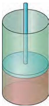
- Cylinder pressure If gas in a cylinder is maintained at a constant temperature T, the pressure P is related to the volume V by a formula of the form
in which a, b, n, and R are constants. Find dP/dV. (See accompanying figure.)
- The best quantity to order One of the formulas for inventory management says that the average weekly cost of ordering, paying for, and holding merchandise is
where q is the quantity you order when things run low (shoes, TVs, brooms, or whatever the item might be); k is the cost of placing an order (the same, no matter how often you order); c is the cost of one item (a constant); m is the number of items sold each week (a constant); and h is the weekly holding cost per item (a constant that takes into account things such as space, utilities, insurance, and security). Find dA/dq and
3.4 The Derivative as a Rate of Change
In this section we study applications where derivatives model the rates at which things change. It is natural to think of a quantity changing with respect to time, but other variables can be treated in the same way. For example, an economist may want to study how the cost of producing steel varies with the number of tons produced, or an engineer may want to know how the power output of a generator varies with its temperature.
Instantaneous Rates of Change
If we interpret the difference quotient
DEFINITION The instantaneous rate of change of f with respect to x at
is the derivative 𝑥 0 𝑓 ′ ( 𝑥 0 ) = l i m ℎ → 0 𝑓 ( 𝑥 0 + ℎ ) − 𝑓 ( 𝑥 0 ) ℎ , provided the limit exists.
Thus, instantaneous rates are limits of average rates.
It is conventional to use the word instantaneous even when x does not represent time. The word is, however, frequently omitted. When we say rate of change, we mean instantaneous rate of change.
EXAMPLE 1 The area A of a circle is related to its diameter by the equation
How fast does the area change with respect to the diameter when the diameter is 10 m?
Solution The rate of change of the area with respect to the diameter is
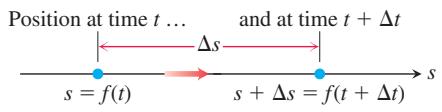
FIGURE 3.15 The positions of a body moving along a coordinate line at time t and shortly later at time
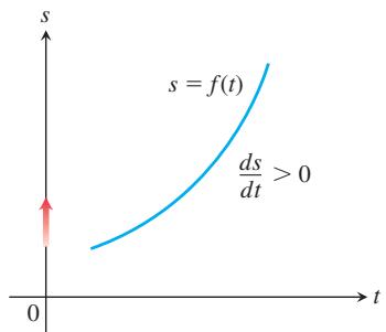
(a) s increasing: positive slope so moving upward
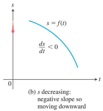
FIGURE 3.16 For motion
When D = 10 m, the area is changing with respect to the diameter at the rate of
Motion Along a Line: Displacement, Velocity, Speed, Acceleration, and Jerk
Suppose that an object (or body, considered as a whole mass) is moving along a coordinate line (an s-axis), usually horizontal or vertical, so that we know its position s on that line as a function of time t:
The displacement of the object over the time interval from t to
and the average velocity of the object over that time interval is
To find the body’s velocity at the exact instant
DEFINITION Velocity (instantaneous velocity) is the derivative of position with respect to time. If a body’s position at time
is 𝑡 , then the body’s velocity at time 𝑠 = 𝑓 ( 𝑡 ) is 𝑡 𝑣 ( 𝑡 ) = 𝑑 𝑠 𝑑 𝑡 = l i m Δ 𝑡 → 0 𝑓 ( 𝑡 + Δ 𝑡 ) − 𝑓 ( 𝑡 ) Δ 𝑡 .
Besides telling how fast an object is moving along the horizontal line in Figure 3.15, its velocity tells the direction of motion. When the object is moving forward (s increasing), the velocity is positive; when the object is moving backward (s decreasing), the velocity is negative. If the coordinate line is vertical, the object moves upward for positive velocity and downward for negative velocity. The blue curves in Figure 3.16 represent position along the line over time; they do not portray the path of motion, which lies along the vertical s-axis.
If we drive to a friend’s house and back at
DEFINITION Speed is the absolute value of velocity.
S p e e d = | 𝑣 ( 𝑡 ) | = ∣ 𝑑 𝑠 𝑑 𝑡 ∣
EXAMPLE 2 Figure 3.17 shows the graph of the velocity
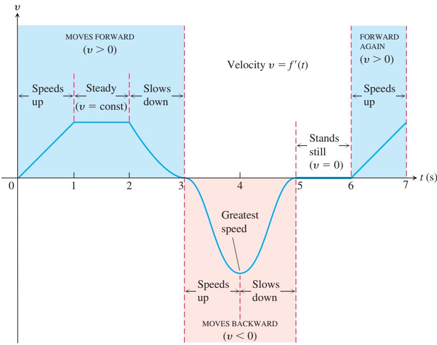
FIGURE 3.17 The velocity graph of a particle moving along a horizontal line, discussed in Example 2.
HISTORICAL BIOGRAPHY Bernard Bolzano (1781–1848) Bolzano was born in Prague, Czechoslovakia. He studied at the University of Prague, where he took courses in philosophy, physics, and mathematics.
To know more, visit the companion Website.
slope of the curve that tells us whether the particle is moving forward or backward along the line (which is not shown in the figure), but rather the sign of the velocity. Figure 3.17 shows that the particle moves forward for the first 3 s (when the velocity is positive), moves backward for the next 2 s (the velocity is negative), stands motionless for a full second, and then moves forward again. The particle is speeding up when its positive velocity increases during the first second, moves at a steady speed during the next second, and then slows down as the velocity decreases to zero during the third second. It stops for an instant at t = 3 s (when the velocity is zero) and reverses direction as the velocity starts to become negative. The particle is now moving backward and gaining in speed until t = 4 s, at which time it achieves its greatest speed during its backward motion. Continuing its backward motion at time t = 4, the particle starts to slow down again until it finally stops at time t = 5 (when the velocity is once again zero). The particle now remains motionless for one full second, and then moves forward again at t = 6 s, speeding up during the final second of the forward motion indicated in the velocity graph.
The rate at which a body’s velocity changes is the body’s acceleration. The acceleration measures how quickly the body picks up or loses speed. In Chapter 12 we will study motion in the plane and in space, where acceleration of an object may also lead to a change in direction.
A sudden change in acceleration is called a jerk. When a ride in a car or a bus is jerky, it is not that the accelerations involved are necessarily large but that the changes in acceleration are abrupt.
DEFINITIONS Acceleration is the derivative of velocity with respect to time. If a body’s position at time
is 𝑡 , then the body’s acceleration at time 𝑠 = 𝑓 ( 𝑡 ) is 𝑡 𝑎 ( 𝑡 ) = 𝑑 𝑣 𝑑 𝑡 = 𝑑 2 𝑠 𝑑 𝑡 2 . Jerk is the derivative of acceleration with respect to time:
𝑗 ( 𝑡 ) = 𝑑 𝑎 𝑑 𝑡 = 𝑑 3 𝑠 𝑑 𝑡 3 .
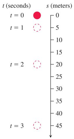
FIGURE 3.18 A ball bearing falling from rest (Example 3).
Near the surface of Earth, all bodies fall with the same constant acceleration. Galileo’s experiments with free fall (see Section 2.1) lead to the equation
where
The value of
The jerk associated with the constant acceleration of gravity (
An object does not exhibit jerkiness during free fall.
EXAMPLE 3 Figure 3.18 shows the free fall of a heavy ball bearing released from rest at time t = 0 s.
(a) How many meters does the ball fall in the first 3 s?
(b) What are its velocity, speed, and acceleration when t = 3?
Solution
(a) The metric free-fall equation is
(b) At any time t, velocity is the derivative of position:
At
in the downward (increasing s) direction. The speed at t = 3 is
The acceleration at any time t is
At t = 3, the acceleration is
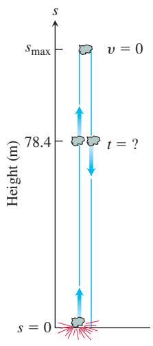
EXAMPLE 4 A dynamite blast blows a heavy rock straight up with a launch velocity of 49 m/s (176.4 km/h) (Figure 3.19a). It reaches a height of
(a) How high does the rock go?
(b) What are the velocity and speed of the rock when it is 78.4 m above the ground on the way up? On the way down?
(c) What is the acceleration of the rock at any time t during its flight (after the blast)?
(d) When does the rock hit the ground again?
(a)
(b)
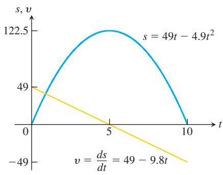
FIGURE 3.19 (a) The rock in Example 4. (b) The graphs of
Solution
(a) In the coordinate system we have chosen, s measures height from the ground up, so the velocity is positive on the way up and negative on the way down. The instant the rock is at its highest point is the one instant during the flight when the velocity is 0. To find the maximum height, all we need to do is to find when v = 0 and evaluate s at this time.
At any time
The velocity is zero when
The rock’s height at
See Figure 3.19b.
(b) To find the rock’s velocity at
To solve this equation, we write
The rock is
At both instants, the rock’s speed is
(c) At any time during its flight following the explosion, the rock’s acceleration is a constant
The acceleration is always downward and is the effect of gravity on the rock. As the rock rises, it slows down; as it falls, it speeds up.
(d) The rock hits the ground at the positive time t for which s = 0. The equation
Derivatives in Economics and Biology
Economists have a specialized vocabulary for rates of change and derivatives. They call them marginals. In a manufacturing operation, the cost of production
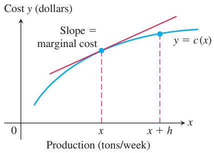
FIGURE 3.20 Weekly steel production:
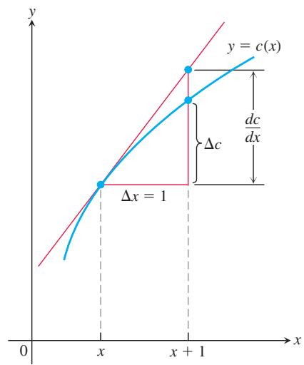
FIGURE 3.21 The marginal cost dc/dx is approximately the extra cost
Suppose that
The limit of this ratio as
Sometimes the marginal cost of production is loosely defined to be the extra cost of producing one additional unit:
which is approximated by the value of dc/dx at x. This approximation is acceptable if the slope of the graph of c does not change quickly near x. Then the difference quotient will be close to its limit dc/dx, which is the rise in the tangent line if
Economists often represent a total cost function by a cubic polynomial
where
EXAMPLE 5 Suppose that it costs
dollars to produce x radiators when 8 to 30 radiators are produced and that
gives the dollar revenue from selling x radiators. Your shop currently produces 10 radiators a day. About how much extra will it cost to produce one more radiator a day, and what is your estimated increase in revenue and increase in profit for selling 11 radiators a day?
Solution The cost of producing one more radiator a day when 10 are produced is about
The additional cost will be about $195. The marginal revenue is
The marginal revenue function estimates the increase in revenue that will result from selling one additional unit. If you currently sell 10 radiators a day, you can expect your revenue to increase by about
if you increase sales to 11 radiators a day. The estimated increase in profit is obtained by subtracting the increased cost of
(a)
EXAMPLE 6 Marginal rates frequently arise in discussions of tax rates. If your marginal income tax rate is 28% and your income increases by
Sensitivity to Change
When a small change in x produces a large change in the value of a function
EXAMPLE 7 Genetic Data and Sensitivity to Change
The Austrian monk Gregor Johann Mendel (1822–1884), working with garden peas and other plants, provided the first scientific explanation of hybridization.
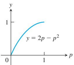
His careful records showed that if p (a number between 0 and 1) is the frequency of the gene for smooth skin in peas (dominant) and
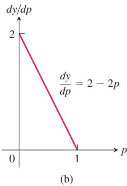
The graph of y versus p in Figure 3.22a suggests that the value of y is more sensitive to a change in p when p is small than when p is large. Indeed, this fact is borne out by the derivative graph in Figure 3.22b, which shows that dy/dp is close to 2 when p is near 0 and close to 0 when p is near 1.
FIGURE 3.22 (a) The graph of
The implication for genetics is that introducing a few more smooth skin genes into a population where the frequency of wrinkled-skin peas is large will have a more dramatic effect on later generations than will a similar increase when the population has a large proportion of smooth-skin peas.
EXERCISES 3.4
Motion Along a Coordinate Line
Exercises 1–6 give the positions
a. Find the body’s displacement and average velocity for the given time interval.
b. Find the body’s speed and acceleration at the endpoints of the interval.
c. When, if ever, during the interval does the body change direction?
-
𝑠 = 𝑡 2 − 3 𝑡 + 2 , 0 ≤ 𝑡 ≤ 2 -
𝑠 = 6 𝑡 − 𝑡 2 , 0 ≤ 𝑡 ≤ 6 -
𝑠 = − 𝑡 3 + 3 𝑡 2 − 3 𝑡 , 0 ≤ 𝑡 ≤ 3 -
𝑠 = ( 𝑡 4 / 4 ) − 𝑡 3 + 𝑡 2 , 0 ≤ 𝑡 ≤ 3 -
𝑠 = 2 5 𝑡 2 − 5 𝑡 , 1 ≤ 𝑡 ≤ 5 𝟔 . 𝑠 = 2 5 𝑡 + 5 , − 4 ≤ 𝑡 ≤ 0 -
Particle motion At time t, the position of a body moving along the s-axis is
𝑠 = 𝑡 3 − 6 𝑡 2 + 9 𝑡
a. Find the body’s acceleration each time the velocity is zero.
b. Find the body’s speed each time the acceleration is zero.
c. Find the total distance traveled by the body from t = 0 to t = 2.
- Particle motion At time
𝑡 ≥ 0 𝑣 = 𝑡 2 − 4 𝑡 + 3
a. Find the body’s acceleration each time the velocity is zero.
b. When is the body moving forward? Backward?
c. When is the body’s velocity increasing? Decreasing?
Free-Fall Applications
-
Free fall on Mars and Jupiter The equations for free fall at the surfaces of Mars and Jupiter (s in meters, t in seconds) are
𝑠 = 1 . 8 6 𝑡 2 𝑠 = 1 1 . 4 4 𝑡 2 -
Lunar projectile motion A rock thrown vertically upward from the surface of the moon at a velocity of 24 m/s (about 86 km/h) reaches a height of s = 24t - 0.8t
2
a. Find the rock’s velocity and acceleration at time
b. How long does it take the rock to reach its highest point?
c. How high does the rock go?
d. How long does it take the rock to reach half its maximum height?
e. How long is the rock aloft?
-
Finding
𝑔 1 5 m / s 𝑔 𝑠 m / s 2 𝑠 = 1 5 𝑡 − ( 1 / 2 ) 𝑔 𝑠 𝑡 2 m 𝑡 2 0 s 𝑔 𝑠 -
Speeding bullet A 45-caliber bullet shot straight up from the surface of the moon would reach a height of
𝑠 = 2 5 0 𝑡 − 0 . 8 𝑡 2 𝑠 = 2 5 0 𝑡 − 4 . 9 𝑡 2 -
Free fall from the Tower of Pisa Had Galileo dropped a cannonball from the Tower of Pisa, 56 m above the ground, the ball’s height above the ground t seconds into the fall would have been
𝑠 = 5 6 − 4 . 9 𝑡 2
a. What would have been the ball’s velocity, speed, and acceleration at time
b. About how long would it have taken the ball to hit the ground?
c. What would have been the ball’s velocity at the moment of impact?
- Galileo’s free-fall formula Galileo developed a formula for a body’s velocity during free fall by rolling balls from rest down increasingly steep inclined planks and looking for a limiting formula that would predict a ball’s behavior when the plank was vertical and the ball fell freely; see part (a) of the accompanying figure. He found that, for any given angle of the plank, the ball’s velocity
𝑡 𝑡 𝑣 = 𝑘 𝑡 𝑘
In modern notation—part (b) of the figure—with distance in meters and time in seconds, what Galileo determined by experiment was that, for any given angle
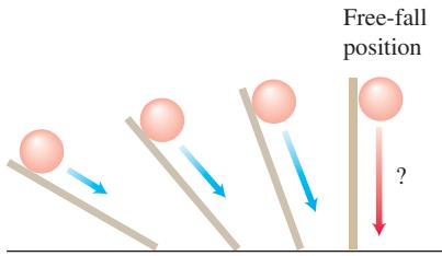
(a)
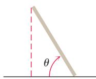
(b)
a. What is the equation for the ball’s velocity during free fall?
b. Building on your work in part (a), what constant acceleration does a freely falling body experience near the surface of Earth?
Understanding Motion from Graphs
- The accompanying figure shows the velocity
𝑣 = 𝑑 𝑠 / 𝑑 𝑡 = 𝑓 ( 𝑡 )
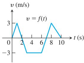
a. When does the body reverse direction?
b. When (approximately) is the body moving at a constant speed?
c. Graph the body’s speed for
d. Graph the acceleration, where defined.
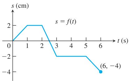
- A particle
𝑃 𝑃 𝑡
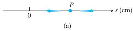
(b)
a. When is
b. Graph the particle’s velocity and speed (where defined).
- Launching a rocket When a model rocket is launched, the propellant burns for a few seconds, accelerating the rocket upward. After burnout, the rocket coasts upward for a while and then begins to fall. A small explosive charge pops out a parachute shortly after the rocket starts down. The parachute slows the rocket to keep it from breaking when it lands.
The figure here shows velocity data from the flight of the model rocket. Use the data to answer the following.
a. How fast was the rocket climbing when the engine stopped?
b. For how many seconds did the engine burn?
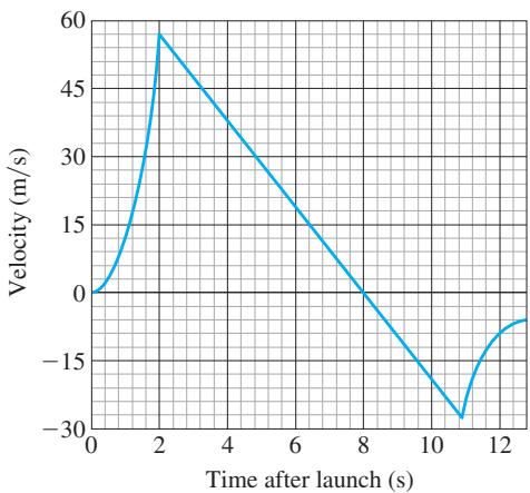
c. When did the rocket reach its highest point? What was its velocity then?
d. When did the parachute pop out? How fast was the rocket falling then?
e. How long did the rocket fall before the parachute opened?
f. When was the rocket’s acceleration greatest?
g. When was the acceleration constant? What was its value then (to the nearest integer)?
- The accompanying figure shows the velocity
𝑣 = 𝑓 ( 𝑡 )
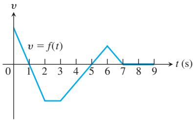
a. When does the particle move forward? Move backward? Speed up? Slow down?
b. When is the particle’s acceleration positive? Negative? Zero?
c. When does the particle move at its greatest speed?
d. When does the particle stand still for more than an instant?
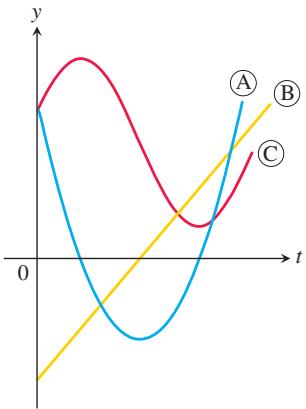
- The graphs in the accompanying figure show the position s, velocity
𝑣 = 𝑑 𝑠 / 𝑑 𝑡 𝑎 = 𝑑 2 𝑠 / 𝑑 𝑡 2
- The graphs in the accompanying figure show the position
𝑠 𝑣 = 𝑑 𝑠 / 𝑑 𝑡 𝑎 = 𝑑 2 𝑠 / 𝑑 𝑡 2 𝑡
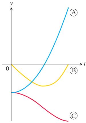
Economics
- Marginal cost Suppose that the dollar cost of producing
𝑥 𝑐 ( 𝑥 ) = 2 0 0 0 + 1 0 0 𝑥 − 0 . 1 𝑥 2
a. Find the average cost per machine of producing the first 100 washing machines.
b. Find the marginal cost when 100 washing machines are produced.
c. Show that the marginal cost when 100 washing machines are produced is approximately the cost of producing one more washing machine after the first 100 have been made, by calculating the latter cost directly.
- Marginal revenue Suppose that the revenue from selling x washing machines is
dollars.
a. Find the marginal revenue when 100 machines are produced.
b. Use the function
c. Find the limit of
Additional Applications
- Bacterium population When a bactericide was added to a nutrient broth in which bacteria were growing, the bacterium population continued to grow for a while, but then stopped growing and began to decline. The size of the population at time t (hours) was
𝑏 = 1 0 6 + 1 0 4 𝑡 − 1 0 3 𝑡 2
a. t = 0 hours.
b. t = 5 hours.
c. t = 10 hours.
-
Body surface area A typical male’s body surface area S in square meters is often modeled by the formula
𝑆 = 1 6 0 √ 𝑤 ℎ -
Draining a tank It takes 12 hours to drain a storage tank by opening the valve at the bottom. The depth y of fluid in the tank t hours after the valve is opened is given by the formula
a. Find the rate
b. When is the fluid level in the tank falling fastest? Slowest? What are the values of
c. Graph y and dy/dt together and discuss the behavior of y in relation to the signs and values of dy/dt.
-
Draining a tank The number of liters of water in a tank t minutes after the tank has started to drain is
𝑄 ( 𝑡 ) = 2 0 0 ( 3 0 − 𝑡 ) 2 -
Vehicular stopping distance Based on data from the U.S. Bureau of Public Roads, a model for the total stopping distance of a moving car in terms of its speed is
where s is measured in meters and v is measured in km/h. The linear term 0.21v models the distance the car travels during the time the driver perceives a need to stop until the brakes are applied, and the quadratic term
- Inflating a balloon The volume
𝑉 = ( 4 / 3 ) 𝜋 𝑟 3
a. At what rate
b. By approximately how much does the volume increase when the radius changes from 2 to 2.2 m?
-
Airplane takeoff Suppose that the distance an aircraft travels along a runway before takeoff is given by
𝐷 = ( 1 0 / 9 ) 𝑡 2 -
Volcanic lava fountains Although the November 1959 Kilauea Iki eruption on the island of Hawaii began with a line of fountains along the wall of the crater, activity was later confined to a single vent in the crater’s floor, which at one point shot lava
5 8 0 m 𝜐 0 𝑠 = 𝑣 0 𝑡 − 4 . 9 𝑡 2
Analyzing Motion Using Graphs
T Exercises 31–34 give the position function
a. When is the object momentarily at rest?
b. When does it move to the left (down) or to the right (up)?
c. When does it change direction?
d. When does it speed up and slow down?
e. When is it moving fastest (highest speed)? Slowest?
f. When is it farthest from the axis origin?
-
𝑠 = 6 0 𝑡 − 4 . 9 𝑡 2 0 ≤ 𝑡 ≤ 1 2 . 5 6 0 m / s -
𝑠 = 𝑡 2 − 3 𝑡 + 2 , 0 ≤ 𝑡 ≤ 5 -
𝑠 = 𝑡 3 − 6 𝑡 2 + 7 𝑡 , 0 ≤ 𝑡 ≤ 4 -
𝑠 = 4 − 7 𝑡 + 6 𝑡 2 − 𝑡 3 , 0 ≤ 𝑡 ≤ 4
3.5 Derivatives of Trigonometric Functions
Many phenomena of nature are approximately periodic (electromagnetic fields, heart rhythms, tides, weather). The derivatives of sines and cosines play a key role in describing periodic changes. This section shows how to differentiate the six basic trigonometric functions.
Derivative of the Sine Function
To calculate the derivative of
If
The derivative of the sine function is the cosine function:
EXAMPLE 1 We find derivatives of a difference, a product, and a quotient, each of which involves the sine function.
Derivative of the Cosine Function
With the help of the angle sum formula for the cosine function (see Figure 1.46),
we can compute the limit of the difference quotient:
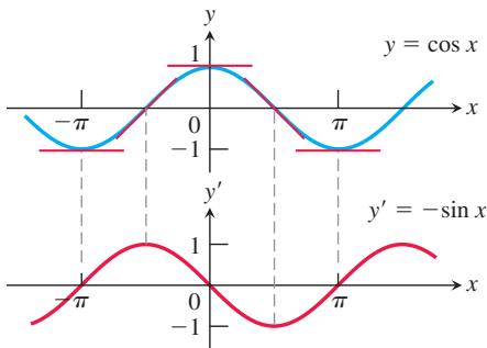
The derivative of the cosine function is the negative of the sine function:
FIGURE 3.23 The curve
Figure 3.23 shows a way to visualize this result by graphing the slopes of the tangent lines to the curve
EXAMPLE 2 We find derivatives of the cosine function in combinations with other functions.
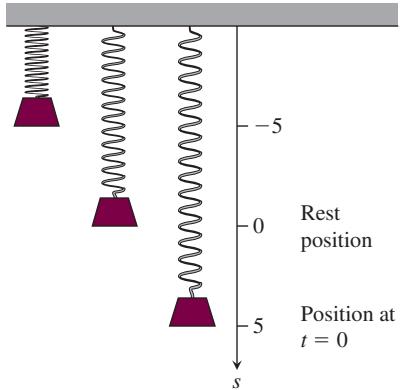
FIGURE 3.24 A weight hanging from a vertical spring and then displaced oscillates above and below its rest position (Example 3).
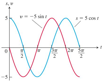
FIGURE 3.25 The graphs of the position and velocity of the weight in Example 3.
(b)
Simple Harmonic Motion
Simple harmonic motion models the motion of an object or weight bobbing freely up and down on the end of a spring, with no resistance. The motion is periodic and repeats indefinitely, so we represent it using trigonometric functions. The next example models motion with no opposing forces (such as friction).
EXAMPLE 3 A weight hanging from a spring (Figure 3.24) is stretched down 5 units beyond its rest position and released at time t = 0 to bob up and down. Its position at any later time t is
What are its velocity and acceleration at time t?
Solution We have
Position:
Velocity:
Acceleration:
Notice how much we can learn from these equations:
-
As time passes, the weight moves down and up between s = -5 and s = 5 on the s-axis. The amplitude of the motion is 5. The period of the motion is
2 𝜋 -
The velocity
𝑣 = − 5 s i n 𝑡 c o s 𝑡 = 0 | 𝑣 | = 5 | s i n 𝑡 | c o s 𝑡 = 0 s i n 𝑡 = 0 𝑠 = 5 c o s 𝑡 = ± 5 -
The weight is acted on by the spring and by gravity. When the weight is below the rest position, the combined forces pull it up, and when it is above the rest position, they pull it down. The weight’s acceleration is always proportional to the negative of its displacement. This property of springs is called Hooke’s Law, and is studied further in Section 6.5.
-
The acceleration,
𝑎 = − 5 c o s 𝑡 c o s 𝑡 = 0 c o s 𝑡 = ± 1
EXAMPLE 4 The jerk associated with the simple harmonic motion in Example 3 is
It has its greatest magnitude when
Derivatives of the Other Basic Trigonometric Functions
Because
are differentiable at every value of x at which they are defined. Their derivatives are given by the following formulas. Notice the negative signs in the derivative formulas for the cofunctions.
The derivatives of the other trigonometric functions:
To show a typical calculation, we find the derivative of the tangent function. The other derivations are left for Exercise 54.
EXAMPLE 5 Find
Solution We use the Derivative Quotient Rule to calculate the derivative:
EXAMPLE 6 Find
Solution Finding the second derivative involves a combination of trigonometric derivatives.
Derivative rule for secant function
EXERCISES 3.5
Derivatives
In Exercises 1–18, find dy/dx.
-
𝑦 = − 1 0 𝑥 + 3 c o s 𝑥 -
𝑦 = 3 𝑥 + 5 s i n 𝑥 -
𝑦 = 𝑥 2 c o s 𝑥 -
𝑦 = √ 𝑥 s e c 𝑥 + 3 -
𝑦 = c s c 𝑥 − 4 √ 𝑥 + 7 𝑒 𝑥 -
𝑦 = 𝑥 2 c o t 𝑥 − 1 𝑥 2 -
𝑓 ( 𝑥 ) = s i n 𝑥 t a n 𝑥 -
𝑔 ( 𝑥 ) = c o s 𝑥 s i n 2 𝑥 -
𝑦 = 𝑥 𝑒 − 𝑥 s e c 𝑥 -
𝑦 = ( s i n 𝑥 + c o s 𝑥 ) s e c 𝑥 -
𝑦 = c o t 𝑥 1 + c o t 𝑥 -
𝑦 = c o s 𝑥 1 + s i n 𝑥 -
𝑦 = 4 c o s 𝑥 + 1 t a n 𝑥 -
𝑦 = c o s 𝑥 𝑥 + 𝑥 c o s 𝑥 -
𝑦 = ( s e c 𝑥 + t a n 𝑥 ) ( s e c 𝑥 − t a n 𝑥 ) -
𝑦 = 𝑥 2 c o s 𝑥 − 2 𝑥 s i n 𝑥 − 2 c o s 𝑥 -
𝑓 ( 𝑥 ) = 𝑥 3 s i n 𝑥 c o s 𝑥 -
𝑔 ( 𝑥 ) = ( 2 − 𝑥 ) t a n 2 𝑥
In Exercises 19–22, find ds/dt.
-
𝑠 = t a n 𝑡 − 𝑒 − 𝑡 -
𝑠 = 𝑡 2 − s e c 𝑡 + 5 𝑒 𝑡 -
𝑠 = 1 + c s c 𝑡 1 − c s c 𝑡 -
𝑠 = s i n 𝑡 1 − c o s 𝑡
In Exercises 23–26, find dr/dθ.
-
𝑟 = 4 − 𝜃 2 s i n 𝜃 -
𝑟 = 𝜃 s i n 𝜃 + c o s 𝜃 -
𝑟 = s e c 𝜃 c s c 𝜃 -
𝑟 = ( 1 + s e c 𝜃 ) s i n 𝜃
In Exercises 27–32, find dp/dq.
-
𝑝 = 5 + 1 c o t 𝑞 -
𝑝 = ( 1 + c s c 𝑞 ) c o s 𝑞 -
𝑝 = s i n 𝑞 + c o s 𝑞 c o s 𝑞 -
𝑝 = t a n 𝑞 1 + t a n 𝑞 -
𝑝 = 𝑞 s i n 𝑞 𝑞 2 − 1 -
𝑝 = 3 𝑞 + t a n 𝑞 𝑞 s e c 𝑞 -
Find
𝑦 ″ 𝑦 = c s c 𝑥 𝑦 = s e c 𝑥 -
Find
𝑦 ( 4 ) = 𝑑 4 𝑦 / 𝑑 𝑥 4 𝑦 = − 2 s i n 𝑥 𝑦 = 9 c o s 𝑥
Tangent Lines
In Exercises 35–38, graph the curves over the given intervals, together with their tangent lines at the given values of x. Label each curve and tangent line with its equation.
-
𝑦 = s i n 𝑥 , − 3 𝜋 / 2 ≤ 𝑥 ≤ 2 𝜋 𝑥 = − 𝜋 , 0 , 3 𝜋 / 2 -
𝑦 = t a n 𝑥 , − 𝜋 / 2 < 𝑥 < 𝜋 / 2 𝑥 = − 𝜋 / 3 , 0 , 𝜋 / 3 -
𝑦 = s e c 𝑥 , − 𝜋 / 2 < 𝑥 < 𝜋 / 2 𝑥 = − 𝜋 / 3 , 𝜋 / 4 -
𝑦 = 1 + c o s 𝑥 , − 3 𝜋 / 2 ≤ 𝑥 ≤ 2 𝜋 𝑥 = − 𝜋 / 3 , 3 𝜋 / 2
Do the graphs of the functions in Exercises 39–44 have any horizontal tangent lines in the interval
-
𝑦 = 𝑥 + s i n 𝑥 -
𝑦 = 2 𝑥 + s i n 𝑥 -
𝑦 = 𝑥 − c o t 𝑥 -
𝑦 = 𝑥 + 2 c o s 𝑥 -
𝑦 = s e c 𝑥 3 + s e c 𝑥 -
𝑦 = c o s 𝑥 3 − 4 s i n 𝑥 -
Find all points on the curve
𝑦 = t a n 𝑥 , − 𝜋 / 2 < 𝑥 < 𝜋 / 2 -
Find all points on the curve
𝑦 = c o t 𝑥 , 0 < 𝑥 < 𝜋
In Exercises 47 and 48, find an equation for (a) the tangent line to the curve at P and (b) the horizontal tangent line to the curve at Q.
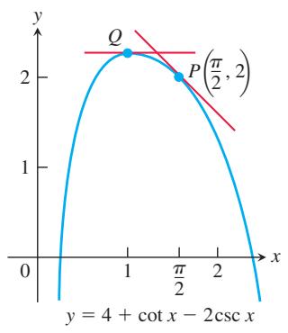
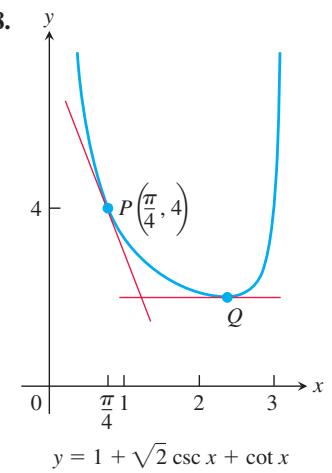
Theory and Examples
The equations in Exercises 49 and 50 give the position
-
𝑠 = 2 − 2 s i n 𝑡 -
𝑠 = s i n 𝑡 + c o s 𝑡 -
Is there a value of c that will make
continuous at
- Is there a value of b that will make
continuous at
- By computing the first few derivatives and looking for a pattern, find the following derivatives.
- Derive the formula for the derivative with respect to
𝑥
a.
- A weight is attached to a spring and reaches its equilibrium position (x = 0). It is then set in motion resulting in a displacement of
where x is measured in centimeters and t is measured in seconds. See the accompanying figure.
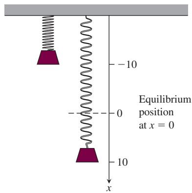
a. Find the spring’s displacement when
b. Find the spring’s velocity when
- Assume that a particle’s position on the
𝑥
where
a. Find the particle’s position when
b. Find the particle’s velocity when
T 57. Graph
for h = 1, 0.5, 0.3, and 0.1. Then, in a new window, try h = -1, -0.5, and -0.3. What happens as
T 58. Graph
for
T 59. Centered difference quotients The centered difference quotient
is used to approximate
See the accompanying figure.
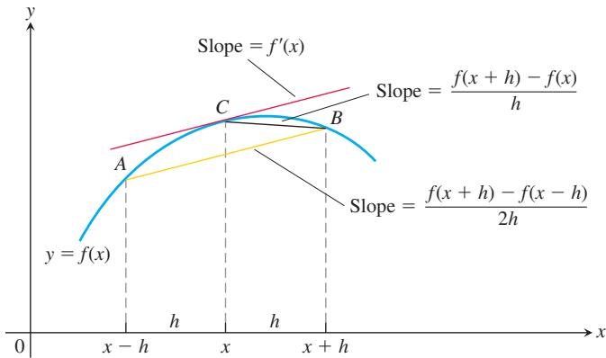
a. To see how rapidly the centered difference quotient for
over the interval
b. To see how rapidly the centered difference quotient for
over the interval
- A caution about centered difference quotients (Continuation of Exercise 59.) The quotient
may have a limit as
As you will see, the limit exists even though
-
Slopes on the graph of the tangent function Graph
𝑦 = t a n 𝑥 ( − 𝜋 / 2 , 𝜋 / 2 ) -
Exploring
( s i n 𝑘 𝑥 ) / 𝑥 𝑦 = ( s i n 𝑥 ) / 𝑥 𝑦 = ( s i n 2 𝑥 ) / 𝑥 𝑦 = ( s i n 4 𝑥 ) / 𝑥 − 2 ≤ 𝑥 ≤ 2 𝑦 = ( s i n 5 𝑥 ) / 𝑥 𝑦 = ( s i n ( − 3 𝑥 ) ) / 𝑥 𝑥 → 0 𝑦 = ( s i n 𝑘 𝑥 ) / 𝑥
3.6 The Chain Rule
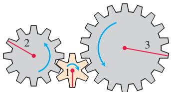
C: y turns B: u turns A: x turns
FIGURE 3.26 When gear A makes
How do we differentiate
Derivative of a Composite Function
The function
Since
If we think of the derivative as a rate of change, this relationship is intuitively reasonable. If
EXAMPLE 1 The function
is obtained by composing the functions
Calculating the derivative from the expanded formula
The derivative of the composite function
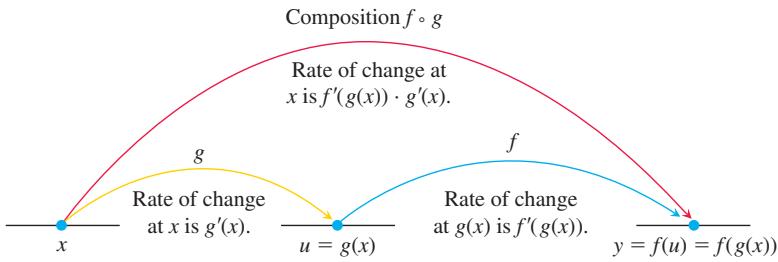
FIGURE 3.27 Rates of change multiply: The derivative of
THEOREM 2—The Chain Rule If
In Leibniz’s notation, if
where
A Proof of One Case of the Chain Rule: Let
Then the corresponding change in
If
and take the limit as
The problem with this argument is that if the function
EXAMPLE 2 An object moves along the x-axis so that its position at any time
Solution We know that the velocity is dx/dt. In this instance, x is a composition of two functions:
Ways to Write the Chain Rule
By the Chain Rule,
“Outside-Inside” Rule
A difficulty with the Leibniz notation is that it doesn’t state specifically where the derivatives in the Chain Rule are supposed to be evaluated. So it sometimes helps to write the Chain Rule using functional notation. If
In words, differentiate the “outside” function f and evaluate this derivative at the “inside” function
EXAMPLE 3 Differentiate
Solution We apply the Chain Rule directly and find
EXAMPLE 4 Differentiate
Solution Here the inside function is
Generalizing Example 4, we see that the Chain Rule gives the formula
For example,
and
Repeated Use of the Chain Rule
We sometimes have to use the Chain Rule two or more times to find a derivative.
HISTORICAL BIOGRAPHY
Johann Bernoulli (1667–1748)
Johann Bernoulli was born in Switzerland and attended the University of Basel. His doctoral dissertation was in mathematics despite its medical title, which was used to hide his mathematical work from his father who wanted Johann to become a doctor.
To know more, visit the companion Website.
EXAMPLE 5 Find the derivative of
Solution Notice here that the tangent is a function of
The Chain Rule with Powers of a Function
If n is any real number and f is a power function,
EXAMPLE 6 The Power Chain Rule simplifies computing the derivative of a power of an expression.
In part (b) we could also find the derivative with the Quotient Rule.
Power Chain Rule with
because
EXAMPLE 7 In Example 4 of Section 3.2 we saw that the absolute value function
Derivative of the Absolute Value Function
EXAMPLE 8 Show that the slope of every line tangent to the curve
Solution We find the derivative:
At any point
which is the quotient of two positive numbers.
EXAMPLE 9 The formulas for the derivatives of both
By the Chain Rule,
See Figure 3.28. Similarly, the derivative of
The factor
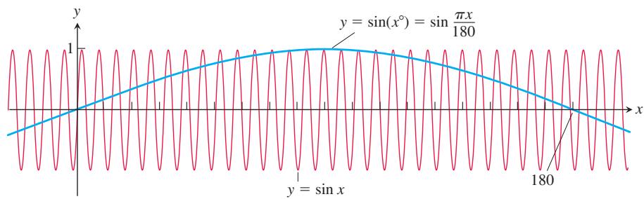
FIGURE 3.28 The function
EXERCISES 3.6
Derivative Calculations
In Exercises 1–8, given
-
𝑦 = 6 𝑢 − 9 , 𝑢 = ( 1 / 2 ) 𝑥 4 -
𝑦 = 2 𝑢 3 , 𝑢 = 8 𝑥 − 1 -
𝑦 = s i n 𝑢 , 𝑢 = 3 𝑥 + 1 -
𝑦 = c o s 𝑢 , 𝑢 = 𝑒 − 𝑥 -
𝑦 = √ 𝑢 , 𝑢 = s i n 𝑥 -
𝑦 = s i n 𝑢 , 𝑢 = 𝑥 − c o s 𝑥 -
𝑦 = t a n 𝑢 , 𝑢 = 𝜋 𝑥 2 -
𝑦 = − s e c 𝑢 , 𝑢 = 1 𝑥 + 7 𝑥
In Exercises 9–22, write the function in the form
-
𝑦 = ( 2 𝑥 + 1 ) 5 -
𝑦 = ( 4 − 3 𝑥 ) 9 -
𝑦 = ( 1 − 𝑥 7 ) − 7 -
𝑦 = ( √ 𝑥 2 − 1 ) − 1 0 -
𝑦 = ( 𝑥 2 8 + 𝑥 − 1 𝑥 ) 4 -
𝑦 = √ 3 𝑥 2 − 4 𝑥 + 6 -
𝑦 = s e c ( t a n 𝑥 ) -
𝑦 = c o t ( 𝜋 − 1 𝑥 ) -
𝑦 = t a n 3 𝑥 -
𝑦 = 5 c o s − 4 𝑥 -
𝑦 = 𝑒 − 5 𝑥 -
𝑦 = 𝑒 2 𝑥 / 3 -
𝑦 = 𝑒 ( 4 √ 𝑥 + 𝑥 2 )
Find the derivatives of the functions in Exercises 23–50.
-
𝑠 = 4 3 𝜋 s i n 3 𝑡 + 4 5 𝜋 c o s 5 𝑡 -
𝑠 = s i n ( 3 𝜋 𝑡 2 ) + c o s ( 3 𝜋 𝑡 2 ) -
𝑟 = ( c s c 𝜃 + c o t 𝜃 ) − 1 -
𝑟 = 6 ( s e c 𝜃 − t a n 𝜃 ) 3 / 2 -
𝑦 = 𝑥 2 s i n 4 𝑥 + 𝑥 c o s − 2 𝑥 -
𝑦 = 1 𝑥 s i n − 5 𝑥 − 𝑥 3 c o s 3 𝑥 -
𝑦 = 1 1 8 ( 3 𝑥 − 2 ) 6 + ( 4 − 1 2 𝑥 2 ) − 1 -
𝑦 = ( 5 − 2 𝑥 ) − 3 + 1 8 ( 2 𝑥 + 1 ) 4 -
𝑦 = ( 4 𝑥 + 3 ) 4 ( 𝑥 + 1 ) − 3 -
𝑦 = ( 2 𝑥 − 5 ) − 1 ( 𝑥 2 − 5 𝑥 ) 6 -
𝑦 = 𝑥 𝑒 − 𝑥 + 𝑒 𝑥 3 -
𝑦 = ( 1 + 2 𝑥 ) 𝑒 − 2 𝑥 -
𝑦 = ( 𝑥 2 − 2 𝑥 + 2 ) 𝑒 5 𝑥 / 2 -
𝑦 = ( 9 𝑥 2 − 6 𝑥 + 2 ) 𝑒 𝑥 3 -
ℎ ( 𝑥 ) = 𝑥 t a n ( 2 √ 𝑥 ) + 7 -
𝑘 ( 𝑥 ) = 𝑥 2 s e c ( 1 𝑥 ) -
𝑓 ( 𝑥 ) = √ 7 + 𝑥 s e c 𝑥 -
𝑔 ( 𝑥 ) = t a n 3 𝑥 ( 𝑥 + 7 ) 4 -
𝑓 ( 𝜃 ) = ( s i n 𝜃 1 + c o s 𝜃 ) 2 -
𝑔 ( 𝑡 ) = ( 1 + s i n 3 𝑡 3 − 2 𝑡 ) − 1 -
𝑟 = s i n ( 𝜃 2 ) c o s ( 2 𝜃 ) -
𝑟 = s e c √ 𝜃 t a n ( 1 𝜃 ) -
𝑞 = s i n ( 𝑡 √ 𝑡 + 1 ) -
𝑞 = c o t ( s i n 𝑡 𝑡 ) -
𝑦 = c o s ( 𝑒 − 𝜃 2 ) -
𝑦 = 𝜃 3 𝑒 − 2 𝜃 c o s 5 𝜃
In Exercises 51–70, find dy/dt.
-
𝑦 = s i n 2 ( 𝜋 𝑡 − 2 ) -
𝑦 = s e c 2 𝜋 𝑡 -
𝑦 = ( 1 + c o s 2 𝑡 ) − 4 -
𝑦 = ( 1 + c o t ( 𝑡 / 2 ) ) − 2 -
𝑦 = ( 𝑡 t a n 𝑡 ) 1 0 -
𝑦 = ( 𝑡 − 3 / 4 s i n 𝑡 ) 4 / 3 -
𝑦 = 𝑒 c o s 2 ( 𝜋 𝑡 − 1 ) -
𝑦 = ( 𝑒 s i n ( 𝑡 / 2 ) ) 3 -
𝑦 = ( 𝑡 2 𝑡 3 − 4 𝑡 ) 3 -
𝑦 = ( 3 𝑡 − 4 5 𝑡 + 2 ) − 5 -
𝑦 = s i n ( c o s ( 2 𝑡 − 5 ) ) -
𝑦 = c o s ( 5 s i n ( 𝑡 3 ) ) -
𝑦 = ( 1 + t a n 4 ( 𝑡 1 2 ) ) 3 -
𝑦 = 1 6 ( 1 + c o s 2 ( 7 𝑡 ) ) 3 -
𝑦 = √ 1 + c o s ( 𝑡 2 ) -
𝑦 = 4 s i n ( √ 1 + √ 𝑡 ) -
𝑦 = t a n 2 ( s i n 3 𝑡 ) -
𝑦 = c o s 4 ( s e c 2 3 𝑡 ) -
𝑦 = 3 𝑡 ( 2 𝑡 2 − 5 ) 4 -
𝑦 = √ 3 𝑡 + √ 2 + √ 1 − 𝑡
Second Derivatives
Find
-
𝑦 = ( 1 + 1 𝑥 ) 3 -
𝑦 = ( 1 − √ 𝑥 ) − 1 -
𝑦 = 1 9 c o t ( 3 𝑥 − 1 ) -
𝑦 = 9 t a n ( 𝑥 3 ) -
𝑦 = 𝑥 ( 2 𝑥 + 1 ) 4 -
𝑦 = 𝑥 2 ( 𝑥 3 − 1 ) 5 -
𝑦 = 𝑒 𝑥 2 + 5 𝑥 -
𝑦 = s i n ( 𝑥 2 𝑒 𝑥 )
For each of the following functions, solve both
-
𝑓 ( 𝑥 ) = 𝑥 ( 𝑥 − 4 ) 3 -
𝑓 ( 𝑥 ) = s e c 2 𝑥 − 2 t a n 𝑥 0 ≤ 𝑥 ≤ 2 𝜋
Finding Derivative Values
In Exercises 81–86, find the value of
-
𝑓 ( 𝑢 ) = 𝑢 5 + 1 , 𝑢 = 𝑔 ( 𝑥 ) = √ 𝑥 , 𝑥 = 1 -
𝑓 ( 𝑢 ) = 1 − 1 𝑢 , 𝑢 = 𝑔 ( 𝑥 ) = 1 1 − 𝑥 , 𝑥 = − 1 -
𝑓 ( 𝑢 ) = c o t 𝜋 𝑢 1 0 , 𝑢 = 𝑔 ( 𝑥 ) = 5 √ 𝑥 , 𝑥 = 1 -
𝑓 ( 𝑢 ) = 𝑢 + 1 c o s 2 𝑢 , 𝑢 = 𝑔 ( 𝑥 ) = 𝜋 𝑥 , 𝑥 = 1 / 4 -
𝑓 ( 𝑢 ) = 2 𝑢 𝑢 2 + 1 , 𝑢 = 𝑔 ( 𝑥 ) = 1 0 𝑥 2 + 𝑥 + 1 , 𝑥 = 0 -
𝑓 ( 𝑢 ) = ( 𝑢 − 1 𝑢 + 1 ) 2 , 𝑢 = 𝑔 ( 𝑥 ) = 1 𝑥 2 − 1 , 𝑥 = − 1 -
Assume that
𝑓 ′ ( 3 ) = − 1 𝑔 ′ ( 2 ) = 5 𝑔 ( 2 ) = 3 𝑦 = 𝑓 ( 𝑔 ( 𝑥 ) ) 𝑦 ′ 𝑥 = 2 -
If
𝑟 = s i n ( 𝑓 ( 𝑡 ) ) 𝑓 ( 0 ) = 𝜋 / 3 𝑓 ′ ( 0 ) = 4 𝑑 𝑟 / 𝑑 𝑡 𝑡 = 0 -
Suppose that functions
𝑓 𝑔 𝑥 𝑥 = 2 𝑥 = 3
| x | f(x) | g(x) | f'(x) | g'(x) |
| 2 | 8 | 2 | 1/3 | -3 |
| 3 | 3 | -4 | 2π | 5 |
Find the derivatives with respect to
a.
b.
c.
d.
e.
f.
g.
h.
- Suppose that the functions
𝑓 𝑔 𝑥 𝑥 = 0 𝑥 = 1
| x | f(x) | g(x) | f'(x) | g'(x) |
| 0 | 1 | 1 | 5 | 1/3 |
| 1 | 3 | -4 | -1/3 | -8/3 |
Find the derivatives with respect to x of the following combinations at the given value of x.
a.
c.
d.
e.
f.
g.
-
Find
𝑑 𝑠 / 𝑑 𝑡 𝜃 = 3 𝜋 / 2 𝑠 = c o s 𝜃 𝑑 𝜃 / 𝑑 𝑡 = 5 -
Find dy/dt when x = 1 if
𝑦 = 𝑥 2 + 7 𝑥 − 5
Theory and Examples
What happens if you can write a function as a composition in different ways? Do you get the same derivative each time? The Chain Rule says you should. Try it with the functions in Exercises 93 and 94.
- Find
𝑑 𝑦 / 𝑑 𝑥 𝑦 = 𝑥 𝑦
a.
b.
- Find
𝑑 𝑦 / 𝑑 𝑥 𝑦 = 𝑥 3 / 2 𝑦
a.
b.
-
Find the tangent line to
𝑦 = ( ( 𝑥 − 1 ) / ( 𝑥 + 1 ) ) 2 -
Find the tangent line to
𝑦 = √ 𝑥 2 − 𝑥 + 7 𝑥 = 2 -
a. Find the tangent line to the curve
𝑦 = 2 t a n ( 𝜋 𝑥 / 4 ) 𝑥 = 1
b. Slopes on a tangent curve What is the smallest value the slope of the curve can ever have on the interval
- Slopes on sine curves
a. Find equations for the tangent lines to the curves
b. Can anything be said about the tangent lines to the curves
c. For a given
d. The function
- Running machinery too fast Suppose that a piston is moving straight up and down and that its position at time t seconds is
with
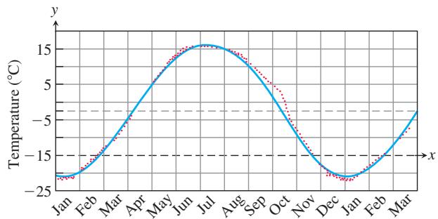
- Temperatures in Fairbanks, Alaska The graph in the accompanying figure shows the average Celsius temperature in Fairbanks, Alaska, during a typical 365-day year. The equation that approximates the temperature on day x is
and is graphed in the accompanying figure.
a. On what day is the temperature increasing the fastest?
b. About how many degrees per day is the temperature increasing when it is increasing at its fastest?
-
Particle motion The position of a particle moving along a coordinate line is
𝑠 = √ 1 + 4 𝑡 -
Constant acceleration Suppose that the velocity of a falling body is
𝑣 = 𝑘 √ 𝑠 m / s 𝑘 𝑠 -
Falling meteorite The velocity of a heavy meteorite entering Earth’s atmosphere is inversely proportional to
√ 𝑠 𝑠 𝑠 2 -
Particle acceleration A particle moves along the
𝑥 𝑑 𝑥 / 𝑑 𝑡 = 𝑓 ( 𝑥 ) 𝑓 ( 𝑥 ) 𝑓 ′ ( 𝑥 ) -
Temperature and the period of a pendulum For oscillations of small amplitude (short swings), we may safely model the relationship between the period T and the length L of a simple pendulum with the equation
where g is the constant acceleration of gravity at the pendulum’s location. If we measure g in centimeters per second squared, we measure L in centimeters and T in seconds. If the pendulum is made of metal, its length will vary with temperature, either increasing or decreasing at a rate that is roughly proportional to L. In symbols, with u being temperature and k the proportionality constant,
Assuming this to be the case, show that the rate at which the period changes with respect to temperature is kT/2.
- Chain Rule Suppose that
𝑓 ( 𝑥 ) = 𝑥 2 𝑔 ( 𝑥 ) = | 𝑥 |
are both differentiable at x = 0 even though g itself is not differentiable at x = 0. Does this contradict the Chain Rule? Explain.
- The derivative of
s i n 2 𝑥 𝑦 = 2 c o s 2 𝑥 − 2 ≤ 𝑥 ≤ 3 . 5
for h = 1.0, 0.5, and 0.2. Experiment with other values of h, including negative values. What do you see happening as
- The derivative of
c o s ( 𝑥 2 ) 𝑦 = − 2 𝑥 s i n ( 𝑥 2 ) − 2 ≤ 𝑥 ≤ 3
for
Using the Chain Rule, show that the Power Rule
a. Show that
b. Determine
c. Show that f is not differentiable at x = 0.
- Consider the function
a. Show that
b. Determine
c. Show that f is not differentiable at x = 0.
d. Show that
- Verify each of the following statements.
a. If
b. If
COMPUTER EXPLORATIONS
Trigonometric Polynomials
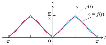
- As the accompanying figure shows, the trigonometric “polynomial”
gives a good approximation of the sawtooth function
a. Graph dg/dt (where defined) over
b. Find
c. Graph df/dt. Where does the approximation of dg/dt by df/dt seem to be best? Least good? Approximations by trigonometric polynomials are important in the theories of heat and oscillation, but we must not expect too much of them, as we see in the next exercise.
- (Continuation of Exercise 114.) In Exercise 114, the trigonometric polynomial
𝑓 ( 𝑡 ) 𝑔 ( 𝑡 ) [ − 𝜋 , 𝜋 ]
graphed in the accompanying figure approximates the step function
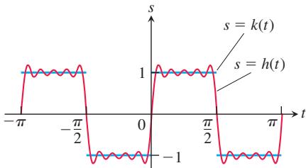
a. Graph dk/dt (where defined) over
b. Find dh/dt.
c. Graph
3.7 Implicit Differentiation
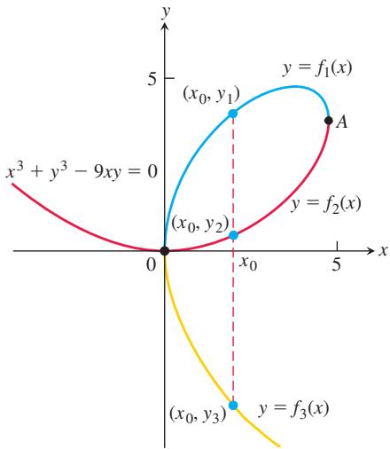
Most of the functions we have dealt with so far have been described by an equation of the form
(See Figures 3.29, 3.30, and 3.31.) Each of these equations defines an implicit relation between the variables x and y, meaning that a value of x may determine more than one value of y, even though we do not have a simple formula for the y-values. In some cases we may be able to solve such an equation for y as an explicit function (or even several functions) of x. When we cannot put an equation
Implicitly Defined Functions
We begin with examples involving familiar equations that we can solve for y as a function of x and then calculate dy/dx in the usual way. Then we differentiate the equations implicitly, and find the derivative. We will see that the two methods give the same answer. Following the examples, we summarize the steps involved in the new method. In the examples and exercises, it is always assumed that the given equation determines y implicitly as a differentiable function of x so that dy/dx exists.
Solution The equation
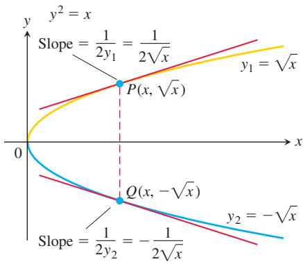
FIGURE 3.30 The equation
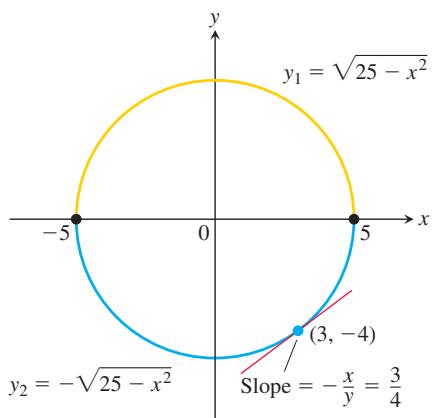
FIGURE 3.31 The circle combines the graphs of two functions. The graph of
But suppose that we knew only that the equation
The answer is yes. To find
This one formula gives the derivatives we calculated for both explicit solutions
EXAMPLE 2 Find the slope of the circle
Solution The circle is not the graph of a single function of x. Rather, it is the combined graphs of two differentiable functions,
We can solve this problem more easily by differentiating the given equation of the circle implicitly with respect to
The slope at
Notice that unlike the slope formula for
To calculate the derivatives of other implicitly defined functions, we proceed as in Examples 1 and 2: We treat y as a differentiable implicit function of x and apply the usual rules to differentiate both sides of the defining equation.
Implicit Differentiation
-
Differentiate both sides of the equation with respect to x, treating y as a differentiable function of x.
-
Collect the terms with dy/dx on one side of the equation and solve for dy/dx.
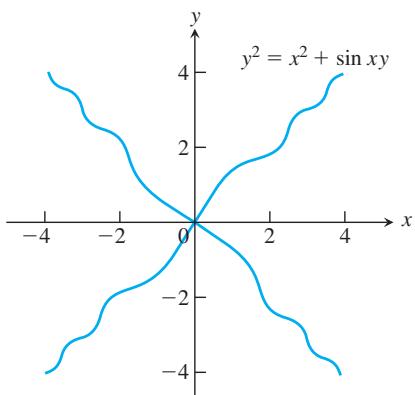
FIGURE 3.32 The graph of the equation in Example 3.
EXAMPLE 3 Find dy/dx if
Solution We differentiate the equation implicitly.
Notice that the formula for dy/dx applies everywhere that the implicitly defined curve has a slope. Notice again that the derivative involves both variables x and y, not just the independent variable x.
Derivatives of Higher Order
Implicit differentiation can also be used to find higher derivatives.
EXAMPLE 4 Find
Solution To start, we differentiate both sides of the equation with respect to x in order to find
We now apply the Quotient Rule to find
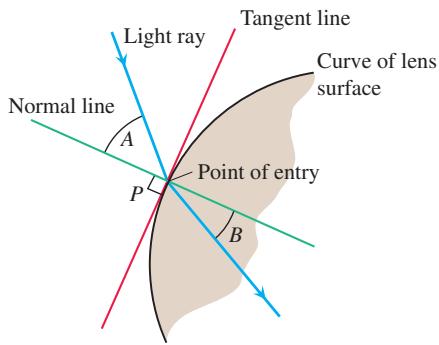
FIGURE 3.33 The profile of a lens, showing the bending (refraction) of a ray of light as it passes through the lens surface.
Finally, we substitute
Lenses, Tangent Lines, and Normal Lines
In the law that describes how light changes direction as it enters a lens, the important angles are the angles the light makes with the line perpendicular to the surface of the lens at the point of entry (angles A and B in Figure 3.33). This line is called the normal line to the surface at the point of entry. In a profile view of a lens like the one in Figure 3.33, the normal line is the line perpendicular (also said to be orthogonal) to the tangent line of the profile curve at the point of entry.
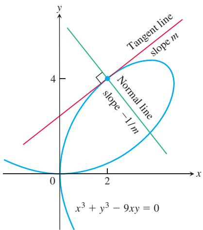
FIGURE 3.34 Example 5 shows how to find equations for the tangent line and normal line to the folium of Descartes at (2, 4).
EXAMPLE 5 Show that the point
Solution The point
To find the slope of the curve at (2,4), we first use implicit differentiation to find a formula for
Differentiate both sides with respect to
Treat xy as a product and y as a function of x.
Solve for dy/dx.
We then evaluate the derivative at
The tangent line at
The normal line to the curve at
Slopes of two nonvertical perpendicular lines are negative reciprocals of each other (see Appendix A.4).
EXERCISES
Differentiating Implicitly
Use implicit differentiation to find
-
𝑥 2 𝑦 + 𝑥 𝑦 2 = 6 -
𝑥 3 + 𝑦 3 = 1 8 𝑥 𝑦 -
2 𝑥 𝑦 + 𝑦 2 = 𝑥 + 𝑦 -
𝑥 3 − 𝑥 𝑦 + 𝑦 3 = 1 -
𝑥 2 ( 𝑥 − 𝑦 ) 2 = 𝑥 2 − 𝑦 2 -
( 3 𝑥 𝑦 + 7 ) 2 = 6 𝑦 -
𝑦 2 = 𝑥 − 1 𝑥 + 1 -
𝑥 3 = 2 𝑥 − 𝑦 𝑥 + 3 𝑦 -
𝑥 = s e c 𝑦 -
𝑥 𝑦 = c o t ( 𝑥 𝑦 ) -
𝑥 + t a n ( 𝑥 𝑦 ) = 0 -
𝑥 4 + s i n 𝑦 = 𝑥 3 𝑦 2 -
𝑦 s i n ( 1 𝑦 ) = 1 − 𝑥 𝑦 -
𝑥 c o s ( 2 𝑥 + 3 𝑦 ) = 𝑦 s i n 𝑥 -
𝑒 2 𝑥 = s i n ( 𝑥 + 3 𝑦 ) -
𝑒 𝑥 2 𝑦 = 2 𝑥 + 2 𝑦
Find
-
𝜃 1 / 2 + 𝑟 1 / 2 = 1 -
𝑟 − 2 √ 𝜃 = 3 2 𝜃 2 / 3 + 4 3 𝜃 3 / 4 -
s i n ( 𝑟 𝜃 ) = 1 2 -
c o s 𝑟 + c o t 𝜃 = 𝑒 𝑟 𝜃
Second Derivatives
In Exercises 21–28, use implicit differentiation to find dy/dx and then
-
𝑥 2 + 𝑦 2 = 1 -
𝑥 2 / 3 + 𝑦 2 / 3 = 1 -
𝑦 2 = 𝑒 𝑥 2 + 2 𝑥 -
𝑦 2 − 2 𝑥 = 1 − 2 𝑦 -
2 √ 𝑦 = 𝑥 − 𝑦 -
𝑥 𝑦 + 𝑦 2 = 1 -
3 + s i n 𝑦 = 𝑦 − 𝑥 3 -
s i n 𝑦 = 𝑥 c o s 𝑦 − 2 -
If
𝑥 3 + 𝑦 3 = 1 6 𝑑 2 𝑦 / 𝑑 𝑥 2 -
If
𝑥 𝑦 + 𝑦 2 = 1 𝑑 2 𝑦 / 𝑑 𝑥 2 ( 0 , − 1 )
In Exercises 31 and 32, find the slope of the curve at the given points.
-
𝑦 2 + 𝑥 2 = 𝑦 4 − 2 𝑥 ( − 2 , 1 ) ( − 2 , − 1 ) -
( 𝑥 2 + 𝑦 2 ) 2 = ( 𝑥 − 𝑦 ) 2 ( 1 , 0 ) ( 1 , − 1 )
Slopes, Tangent Lines, and Normal Lines
In Exercises 33–42, verify that the given point is on the curve and find the lines that are (a) tangent and (b) normal to the curve at the given point.
-
𝑥 2 + 𝑥 𝑦 − 𝑦 2 = 1 , ( 2 , 3 ) -
𝑥 2 + 𝑦 2 = 2 5 -
𝑥 2 𝑦 2 = 9 ( − 1 , 3 ) -
𝑦 2 − 2 𝑥 − 4 𝑦 − 1 = 0 , ( − 2 , 1 ) -
6 𝑥 2 + 3 𝑥 𝑦 + 2 𝑦 2 + 1 7 𝑦 − 6 = 0 , ( − 1 , 0 ) -
𝑥 2 − √ 3 𝑥 𝑦 + 2 𝑦 2 = 5 , ( √ 3 , 2 ) -
2 𝑥 𝑦 + 𝜋 s i n 𝑦 = 2 𝜋 , ( 1 , 𝜋 / 2 ) -
𝑥 s i n 2 𝑦 = 𝑦 c o s 2 𝑥 , ( 𝜋 / 4 , 𝜋 / 2 ) -
𝑦 = 2 s i n ( 𝜋 𝑥 − 𝑦 ) -
𝑥 2 c o s 2 𝑦 − s i n 𝑦 = 0 , ( 0 , 𝜋 ) -
Parallel tangent lines Find the two points where the curve
𝑥 2 + 𝑥 𝑦 + 𝑦 2 = 7 -
Normal lines parallel to a line Find the normal lines to the curve
𝑥 𝑦 + 2 𝑥 − 𝑦 = 0 2 𝑥 + 𝑦 = 0 -
The eight curve Find the slopes of the curve
𝑦 4 = 𝑦 2 − 𝑥 2
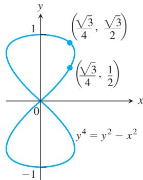
- The cissoid of Diocles (from about 200 B.C.) Find equations for the tangent line and normal line to the cissoid of Diocles
𝑦 2 ( 2 − 𝑥 ) = 𝑥 3
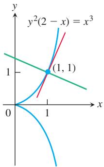
- The devil’s curve (Gabriel Cramer, 1750) Find the slopes of the devil’s curve
𝑦 4 − 4 𝑦 2 = 𝑥 4 − 9 𝑥 2
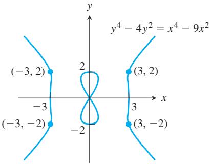
- The folium of Descartes (See Figure 3.29)
a. Find the slope of the folium of Descartes
b. At what point other than the origin does the folium have a horizontal tangent line?
c. Find the coordinates of the point
Theory and Examples
-
Intersecting normal line The line that is normal to the curve
𝑥 2 + 2 𝑥 𝑦 − 3 𝑦 2 = 0 -
Power rule for rational exponents Let
𝑝 𝑞 𝑞 > 0 𝑦 = 𝑥 𝑝 / 𝑞 𝑦 𝑞 = 𝑥 𝑝 𝑦 ≠ 0
- Normal lines to a parabola Show that if it is possible to draw three normal lines from the point
( 𝑎 , 0 ) 𝑥 = 𝑦 2
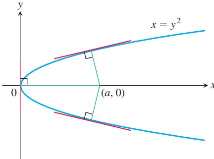
- Is there anything special about the tangent lines to the curves
𝑦 2 = 𝑥 3 2 𝑥 2 + 3 𝑦 2 = 5 ( 1 , ± 1 )
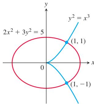
- Verify that the following pairs of curves meet orthogonally.
a.
b.
- The graph of
𝑦 2 = 𝑥 3 𝑏 𝑦 = − 1 3 𝑥 + 𝑏
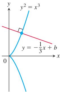
In Exercises 55 and 56, find both dy/dx (treating y as a differentiable function of x) and dx/dy (treating x as a differentiable function of y). How do dy/dx and dx/dy seem to be related?
-
𝑥 𝑦 3 + 𝑥 2 𝑦 = 6 -
𝑥 3 + 𝑦 2 = s i n 2 𝑦 -
Derivative of arcsine Assume that
𝑦 = s i n − 1 𝑥 𝑥 𝑥 = s i n 𝑦 𝑑 𝑦 / 𝑑 𝑥 = 1 / √ 1 − 𝑥 2 -
Use the formula in Exercise 57 to find dy/dx if
a.
b.
COMPUTER EXPLORATIONS
Use a CAS to perform the following steps in Exercises 59–66.
a. Plot the equation with the implicit plotter of a CAS. Check to see that the given point
b. Using implicit differentiation, find a formula for the derivative
c. Use the slope found in part (b) to find an equation for the tangent line to the curve at P. Then plot the implicit curve and tangent line together on a single graph.
-
𝑥 3 − 𝑥 𝑦 + 𝑦 3 = 7 , 𝑃 ( 2 , 1 ) -
𝑥 5 + 𝑦 3 𝑥 + 𝑦 𝑥 2 + 𝑦 4 = 4 , 𝑃 ( 1 , 1 ) -
𝑦 2 + 𝑦 = 2 + 𝑥 1 − 𝑥 , 𝑃 ( 0 , 1 ) -
𝑦 3 + c o s 𝑥 𝑦 = 𝑥 2 , 𝑃 ( 1 , 0 ) -
𝑥 + t a n ( 𝑦 𝑥 ) = 2 , 𝑃 ( 1 , 𝜋 4 ) -
𝑥 𝑦 3 + t a n ( 𝑥 + 𝑦 ) = 1 , 𝑃 ( 𝜋 4 , 0 ) -
2 𝑦 2 + ( 𝑥 𝑦 ) 1 / 3 = 𝑥 2 + 2 , 𝑃 ( 1 , 1 ) -
𝑥 √ 1 + 2 𝑦 + 𝑦 = 𝑥 2 , 𝑃 ( 1 , 0 )
3.8 Derivatives of Inverse Functions and Logarithms
In Section 1.5 we saw how the inverse of a function undoes, or inverts, the effect of that function. We defined there the natural logarithm function
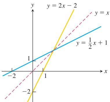
FIGURE 3.35 Graphing a line and its inverse together shows the graphs’ symmetry with respect to the line y = x. The slopes are reciprocals of each other.
Derivatives of Inverses of Differentiable Functions
We calculated the inverse of the function
The derivatives are reciprocals of one another, so the slope of one line is the reciprocal of the slope of its inverse line. (See Figure 3.35.)
This is not a special case. Reflecting any nonhorizontal or nonvertical line across the line y = x always inverts the line’s slope. If the original line has slope
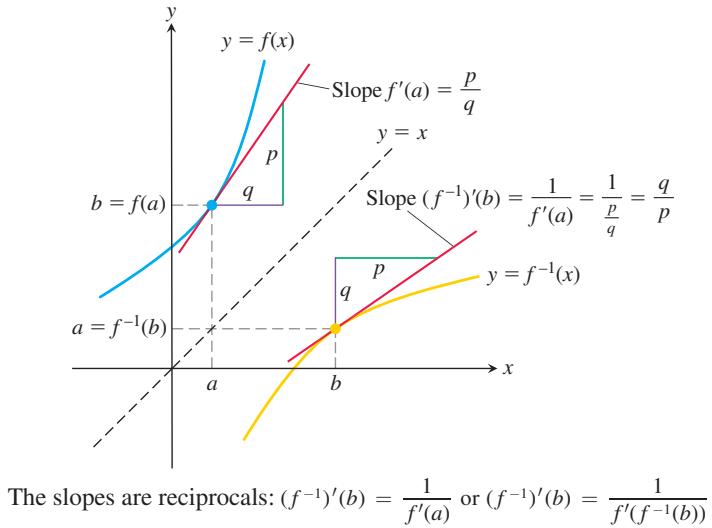
FIGURE 3.36 The graphs of inverse functions have recip-
rocal slopes at corresponding points.
The reciprocal relationship between the slopes of f and
If
THEOREM 3—The Derivative Rule for Inverses
If
or
Theorem 3 makes two assertions. The first of these has to do with the conditions under which
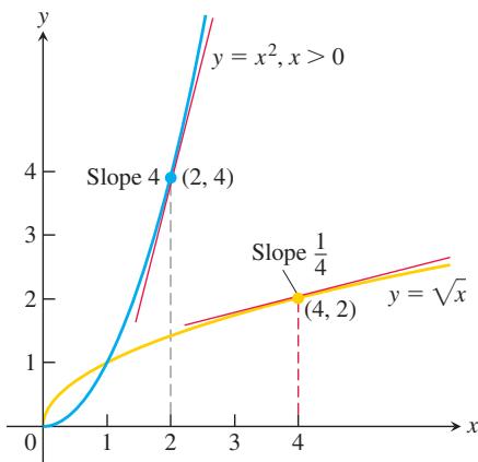
FIGURE 3.37 The derivative of
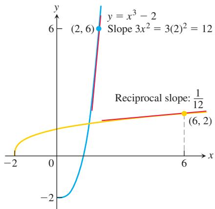
FIGURE 3.38 The derivative of
EXAMPLE 1 The function
Let’s verify that Theorem 3 gives the same formula for the derivative of
Theorem 3 gives a derivative that agrees with the known derivative of the square root function.
Let’s examine Theorem 3 at a specific point. We pick
See Figure 3.37.
We will use the procedure illustrated in Example 1 to calculate formulas for the derivatives of many inverse functions throughout this chapter. Equation (1) sometimes enables us to find specific values of
EXAMPLE 2 Let
Solution We apply Theorem 3 to obtain the value of the derivative of
Derivative of the Natural Logarithm Function
Since we know that the exponential function
Alternative Derivation Instead of applying Theorem 3 directly, we can find the derivative of
No matter which derivation we use, the derivative of
The Chain Rule extends this formula to positive differentiable functions
EXAMPLE 3 We use Equations (2) and (3) to find derivatives.
(b) Equation (3) with
(c) Using the Chain Rule and Equation (2), we find
(d) Equation (3) with
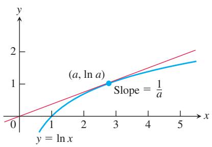
FIGURE 3.39 The tangent line meets the curve at some point
So
Notice from Example 3a that the function
EXAMPLE 4 A line with slope m passes through the origin and is tangent to the graph of
Solution Suppose the point of tangency occurs at the unknown point x = a > 0. Then we know that the point
Setting these two formulas for m equal to each other, we have
The Derivatives of 𝑎 𝑥 l o g 𝑎 𝑥
We start with the equation
That is, if a > 0, then
This equation shows why
If a > 0 and u is a differentiable function of x, then by the Chain Rule,
EXAMPLE 5 Here are some derivatives of general exponential functions.
In Section 3.3 we looked at the derivative
In particular, when
However, we have not fully justified that these limits actually exist. While all of the arguments given in deriving the derivatives of the exponential and logarithmic functions are correct, they do assume the existence of these limits. In Chapter 7 we will give another development of the theory of logarithmic and exponential functions which fully justifies that both limits do in fact exist and have the values derived above.
To find the derivative of
Then we take derivatives
which yields
If
Logarithmic Differentiation
The derivatives of positive functions given by formulas that involve products, quotients, and powers can often be found more quickly if we take the natural logarithm of both sides before differentiating. This enables us to use the laws of logarithms to simplify the formulas before differentiating. The process, called logarithmic differentiation, is illustrated in the next example.
EXAMPLE 6 Find dy/dx if
Solution We take the natural logarithm of both sides and simplify the result with the algebraic properties of logarithms from Theorem 1 in Section 1.5:
We then take derivatives of both sides with respect to x, using Equation (3):
Next we solve for
Finally, we substitute for y:
The computation in Example 6 would be much longer if we used the product, quotient, and power rules.
Irrational Exponents and the Power Rule (General Version)
The natural logarithm and the exponential function will be defined precisely in Chapter 7. We can use the exponential function to define the general exponential function, which enables us to raise any positive number to any real power n, rational or irrational. That is, we can define the power function
DEFINITION For any x > 0 and for any real number n,
𝑥 𝑛 = 𝑒 𝑛 l n 𝑥 .
Because the logarithm and exponential functions are inverses of each other, the definition gives
That is, the rule for taking the natural logarithm of a power holds for all real exponents
The definition of the power function also enables us to establish the derivative Power Rule for any real power n, as stated in Section 3.3.
General Power Rule for Derivatives
For x > 0 and any real number n,
Proof Differentiating 𝑥 𝑛
In short, whenever x > 0,
For
Using implicit differentiation (which assumes the existence of the derivative
Solving for the derivative, we find that
It can be shown directly from the definition of the derivative that the derivative equals 0 when x = 0 and n > 1 (see Exercise 107). This completes the proof of the general version of the Power Rule for all values of x.
EXAMPLE 7 Differentiate
Solution The Power Rule tells us how to differentiate a function of the form
We can also find the derivative of
The Number e Expressed as a Limit
In Section 1.4 we defined the number e as the base value for which the exponential function
We now prove that
THEOREM 4—The Number
Proof If
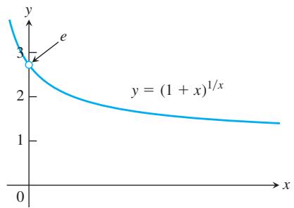
FIGURE 3.40 The number e is the limit of the function graphed here as
Because
Therefore, exponentiating both sides, we get
See Figure 3.40.
Approximating the limit in Theorem 4 by taking x very small gives approximations to e. Its value is
Exercises 3.8
Derivatives of Inverse Functions
In Exercises 1–4:
a. Find
b. Graph
c. Evaluate
-
𝑓 ( 𝑥 ) = 2 𝑥 + 3 , 𝑎 = − 1 -
𝑓 ( 𝑥 ) = 𝑥 + 2 1 − 𝑥 , 𝑎 = 1 2 -
𝑓 ( 𝑥 ) = 5 − 4 𝑥 , 𝑎 = 1 / 2 -
𝑓 ( 𝑥 ) = 2 𝑥 2 , 𝑥 ≥ 0 , 𝑎 = 5 -
a. Show that
𝑓 ( 𝑥 ) = 𝑥 3 𝑔 ( 𝑥 ) = 3 √ 𝑥
b. Graph f and g over an x-interval large enough to show the graphs intersecting at
c. Find the slopes of the tangent lines to the graphs of
d. What lines are tangent to the curves at the origin?
- a. Show that
ℎ ( 𝑥 ) = 𝑥 3 / 4 𝑘 ( 𝑥 ) = ( 4 𝑥 ) 1 / 3
b. Graph h and k over an x-interval large enough to show the graphs intersecting at
c. Find the slopes of the tangent lines to the graphs at h and k at
d. What lines are tangent to the curves at the origin?
-
Let
𝑓 ( 𝑥 ) = 𝑥 3 − 3 𝑥 2 − 1 𝑥 ≥ 2 𝑑 𝑓 − 1 / 𝑑 𝑥 𝑥 = − 1 = 𝑓 ( 3 ) -
Let
𝑓 ( 𝑥 ) = 𝑥 2 − 4 𝑥 − 5 𝑥 > 2 𝑑 𝑓 − 1 / 𝑑 𝑥 𝑥 = 0 = 𝑓 ( 5 ) -
Suppose that the differentiable function
𝑦 = 𝑓 ( 𝑥 ) 𝑑 𝑓 − 1 / 𝑑 𝑥 -
Suppose that the differentiable function
𝑦 = 𝑔 ( 𝑥 ) 𝑔 − 1 -
The accompanying figure shows the graph of the function f.
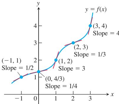
Assuming the inverse function
a.
- The accompanying figure shows the graph of the function g.
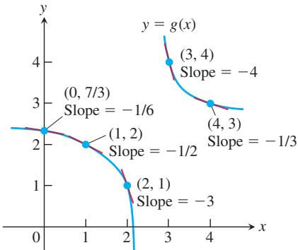
Assuming the inverse function
a.
- Suppose that the function f and its derivative with respect to x have the following values at x = 0, 1, 2, 3, and 4.
| x | 0 | 1 | 2 | 3 | 4 |
| f(x) | 3 | 6 | 0 | 1 | 2 |
| f'(x) | 4/3 | 5 | 4 | 1/2 | 1/7 |
Assuming the inverse function
a.
- Suppose that the function
𝑔 𝑥 𝑥 = 0 , 1 , 2 , 3
| x | 0 | 1 | 2 | 3 | 4 |
| g(x) | -4 | -1 | 1 | 2 | 3 |
| g'(x) | 3 | 2 | 5/4 | 2/3 | 1/5 |
Assuming the inverse function
a.
Derivatives of Logarithms
In Exercises 15–44, find the derivative of y with respect to x, t, or
-
𝑦 = l n 3 𝑥 + 𝑥 -
𝑦 = l n ( 𝑡 2 )
-
𝑦 = l n ( 𝑡 3 / 2 ) + √ 𝑡 -
𝑦 = l n 3 𝑥 -
𝑦 = l n ( s i n 𝑥 ) -
𝑦 = l n ( 𝜃 + 1 ) − 𝑒 𝜃 -
𝑦 = ( c o s 𝜃 ) l n ( 2 𝜃 + 2 ) -
𝑦 = l n 𝑥 3 -
𝑦 = ( l n 𝑥 ) 3 -
𝑦 = 𝑡 ( l n 𝑡 ) 2 -
𝑦 = 𝑡 l n √ 𝑡 -
𝑦 = 𝑥 4 4 l n 𝑥 − 𝑥 4 1 6 -
𝑦 = ( 𝑥 2 l n 𝑥 ) 4 -
𝑦 = l n 𝑡 𝑡 -
𝑦 = 𝑡 √ l n 𝑡 -
𝑦 = l n 𝑥 1 + l n 𝑥 -
𝑦 = 𝑥 l n 𝑥 1 + l n 𝑥 -
𝑦 = l n ( l n 𝑥 ) -
𝑦 = l n ( l n ( l n 𝑥 ) ) -
𝑦 = 𝜃 ( s i n ( l n 𝜃 ) + c o s ( l n 𝜃 ) ) -
𝑦 = l n ( s e c 𝜃 + t a n 𝜃 ) -
𝑦 = l n 1 𝑥 √ 𝑥 + 1 -
𝑦 = 1 2 l n 1 + 𝑥 1 − 𝑥 -
𝑦 = 1 + l n 𝑡 1 − l n 𝑡 -
𝑦 = √ l n √ 𝑡 -
𝑦 = l n ( s e c ( l n 𝜃 ) ) -
𝑦 = l n ( √ s i n 𝜃 c o s 𝜃 1 + 2 l n 𝜃 ) -
𝑦 = l n ( ( 𝑥 2 + 1 ) 5 √ 1 − 𝑥 ) -
𝑦 = l n √ ( 𝑥 + 1 ) 5 ( 𝑥 + 2 ) 2 0
Logarithmic Differentiation
In Exercises 45–58, use logarithmic differentiation to find the derivative of y with respect to the given independent variable.
-
𝑦 = √ 𝑥 ( 𝑥 + 1 ) -
𝑦 = √ ( 𝑥 2 + 1 ) ( 𝑥 − 1 ) 2 -
𝑦 = √ 𝑡 𝑡 + 1 -
𝑦 = √ 1 𝑡 ( 𝑡 + 1 ) -
𝑦 = ( s i n 𝜃 ) √ 𝜃 + 3 -
𝑦 = ( t a n 𝜃 ) √ 2 𝜃 + 1 -
𝑦 = 𝑡 ( 𝑡 + 1 ) ( 𝑡 + 2 ) -
𝑦 = 1 𝑡 ( 𝑡 + 1 ) ( 𝑡 + 2 ) -
𝑦 = 𝜃 + 5 𝜃 c o s 𝜃 -
𝑦 = 𝜃 s i n 𝜃 √ s e c 𝜃 -
𝑦 = 𝑥 √ 𝑥 2 + 1 ( 𝑥 + 1 ) 2 / 3 -
𝑦 = √ ( 𝑥 + 1 ) 1 0 ( 2 𝑥 + 1 ) 5 -
𝑦 = 3 √ 𝑥 ( 𝑥 − 2 ) 𝑥 2 + 1 -
𝑦 = 3 √ 𝑥 ( 𝑥 + 1 ) ( 𝑥 − 2 ) ( 𝑥 2 + 1 ) ( 2 𝑥 + 3 )
Finding Derivatives
In Exercises 59–70, find the derivative of y with respect to x, t, or
-
𝑦 = l n ( c o s 2 𝜃 ) -
𝑦 = l n ( 3 𝜃 𝑒 − 𝜃 ) -
𝑦 = l n ( 3 𝑡 𝑒 − 𝑡 ) -
𝑦 = l n ( 2 𝑒 − 𝑡 s i n 𝑡 ) -
𝑦 = l n ( 𝑒 𝜃 1 + 𝑒 𝜃 ) -
𝑦 = l n ( √ 𝜃 1 + √ 𝜃 ) -
𝑦 = 𝑒 ( c o s 𝑡 + l n 𝑡 ) -
𝑦 = 𝑒 s i n 𝑡 ( l n 𝑡 2 + 1 )
In Exercises 67–70, find dy/dx.
-
l n 𝑦 = 𝑒 𝑦 s i n 𝑥 -
l n 𝑥 𝑦 = 𝑒 𝑥 + 𝑦 -
𝑥 𝑦 = 𝑦 𝑥 -
t a n 𝑦 = 𝑒 𝑥 + l n 𝑥
In Exercises 71–92, find the derivative of y with respect to the given independent variable.
-
𝑦 = 2 𝑥 -
𝑦 = 3 − 𝑥 -
𝑦 = 5 √ 𝑠 -
𝑦 = 2 ( 𝑠 2 ) -
𝑦 = 𝑥 𝜋 -
𝑦 = 𝑡 1 − 𝑒 -
𝑦 = l o g 2 5 𝜃 -
𝑦 = l o g 3 ( 1 + 𝜃 l n 3 ) -
𝑦 = l o g 4 𝑥 + l o g 4 𝑥 2 -
𝑦 = l o g 2 5 𝑒 𝑥 − l o g 5 √ 𝑥 -
𝑦 = l o g 2 𝑟 ⋅ l o g 4 𝑟 -
𝑦 = l o g 3 𝑟 ⋅ l o g 9 𝑟 -
𝑦 = l o g 3 ( ( 𝑥 + 1 𝑥 − 1 ) l n 3 ) -
𝑦 = l o g 5 √ ( 7 𝑥 3 𝑥 + 2 ) l n 5 -
𝑦 = 𝜃 s i n ( l o g 7 𝜃 ) -
𝑦 = l o g 7 ( s i n 𝜃 c o s 𝜃 𝑒 𝜃 2 𝜃 ) -
𝑦 = l o g 5 𝑒 𝑥 -
𝑦 = l o g 2 ( 𝑥 2 𝑒 2 2 √ 𝑥 + 1 ) -
𝑦 = 3 l o g 2 𝑡 -
𝑦 = 3 l o g 8 ( l o g 2 𝑡 ) -
𝑦 = l o g 2 ( 8 𝑡 l n 2 ) -
𝑦 = 𝑡 l o g 3 ( 𝑒 ( s i n 𝑡 ) ( l n 3 ) )
Powers with Variable Bases and Exponents
In Exercises 93–104, use logarithmic differentiation or the method in Example 7 to find the derivative of y with respect to the given independent variable.
-
𝑦 = ( 𝑥 + 1 ) 𝑥 -
𝑦 = 𝑥 ( 𝑥 + 1 ) -
𝑦 = ( √ 𝑡 ) 𝑡 -
𝑦 = 𝑡 √ 𝑡 -
𝑦 = ( s i n 𝑥 ) 𝑥 -
𝑦 = 𝑥 s i n 𝑥 -
𝑦 = 𝑥 l n 𝑥 -
𝑦 = ( l n 𝑥 ) l n 𝑥 -
𝑦 𝑥 = 𝑥 3 𝑦 -
𝑥 s i n 𝑦 = l n 𝑦 -
𝑥 = 𝑦 𝑥 𝑦 -
𝑒 𝑦 = 𝑦 l n 𝑥
Theory and Applications
- If we write
𝑔 ( 𝑥 ) 𝑓 − 1 ( 𝑥 )
If we then write
The latter equation may remind you of the Chain Rule, and indeed there is a connection.
Assume that
-
Show that
l i m 𝑛 → ∞ ( 1 + 𝑥 𝑛 ) 𝑛 = 𝑒 𝑥 𝑥 > 0 -
If
𝑓 ( 𝑥 ) = 𝑥 𝑛 𝑛 > 1 𝑓 ′ ( 0 ) = 0 -
Using mathematical induction, show that for
𝑛 > 1
COMPUTER EXPLORATIONS
In Exercises 109–116, you will explore some functions and their inverses together with their derivatives and tangent line approximations at specified points. Perform the following steps using your CAS:
a. Plot the function
b. Solve the equation
c. Find an equation for the tangent line to
d. Find an equation for the tangent line to
e. Plot the functions f and g, the identity, the two tangent lines, and the line segment joining the points
-
𝑦 = √ 3 𝑥 − 2 , 2 3 ≤ 𝑥 ≤ 4 , 𝑥 0 = 3 -
𝑦 = 3 𝑥 + 2 2 𝑥 − 1 1 , − 2 ≤ 𝑥 ≤ 2 , 𝑥 0 = 1 / 2 -
𝑦 = 4 𝑥 𝑥 2 + 1 , − 1 ≤ 𝑥 ≤ 1 , 𝑥 0 = 1 / 2 -
𝑦 = 𝑥 3 𝑥 2 + 1 , − 1 ≤ 𝑥 ≤ 1 , 𝑥 0 = 1 / 2 -
𝑦 = 𝑥 3 − 3 𝑥 2 − 1 , 2 ≤ 𝑥 ≤ 5 , 𝑥 0 = 2 7 1 0 -
𝑦 = 2 − 𝑥 − 𝑥 3 , − 2 ≤ 𝑥 ≤ 2 , 𝑥 0 = 3 2 -
𝑦 = 𝑒 𝑥 , − 3 ≤ 𝑥 ≤ 5 , 𝑥 0 = 1 -
𝑦 = s i n 𝑥 , − 𝜋 2 ≤ 𝑥 ≤ 𝜋 2 , 𝑥 0 = 1
In Exercises 117 and 118, repeat the steps above to solve for the functions
-
𝑦 1 / 3 − 1 = ( 𝑥 + 2 ) 3 , − 5 ≤ 𝑥 ≤ 5 , 𝑥 0 = − 3 / 2 -
c o s 𝑦 = 𝑥 1 / 5 0 ≤ 𝑥 ≤ 1 𝑥 0 = 1 / 2
3.9 Inverse Trigonometric Functions
We introduced the six basic inverse trigonometric functions in Section 1.5 but focused there on the arcsine and arccosine functions. Here we complete the study of how all six basic inverse trigonometric functions are defined, graphed, and evaluated, and how their derivatives are computed.
Inverses of t a n 𝑥 c o t 𝑥 s e c 𝑥 c s c 𝑥
The graphs of these four basic inverse trigonometric functions are shown in Figure 3.41. We obtain these graphs by reflecting the graphs of the restricted trigonometric functions (as discussed in Section 1.5) through the line
Domain:
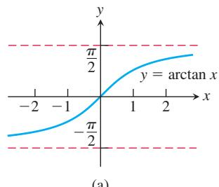
(a)
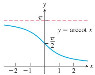
(b)
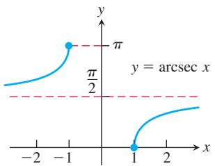
(c)
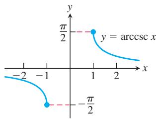
(d)
FIGURE 3.41 Graphs of the arctangent, arccotangent, arcsecant, and arccosecant functions.
The arctangent of x is a radian angle whose tangent is x. The arcotangent of x is an angle whose cotangent is x, and so forth. The angles belong to the restricted domains of the tangent, cotangent, secant, and cosecant functions.
DEFINITIONS
y = arctan x is the number in
for which tan y = x. ( − 𝜋 / 2 , 𝜋 / 2 )
is the number in 𝑦 = a r c c o t 𝑥 for which ( 0 , 𝜋 ) . c o t 𝑦 = 𝑥 y = arcsec x is the number in
for which sec y = x. [ 0 , 𝜋 / 2 ) ∪ ( 𝜋 / 2 , 𝜋 ]
is the number in 𝑦 = a r c c s c 𝑥 for which [ − 𝜋 / 2 , 0 ) ∪ ( 0 , 𝜋 / 2 ] . c s c 𝑦 = 𝑥
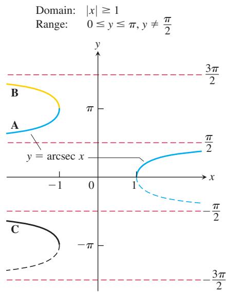
FIGURE 3.42 There are several logical choices for the left-hand branch of
We use open or half-open intervals to avoid values for which the tangent, cotangent, secant, and cosecant functions are undefined. (See Figure 3.41.)
As we discussed in Section 1.5, the arcsine and arccosine functions are often written as
The graph of
the arctangent is an odd function. The graph of y = arccot x has no such symmetry (Figure 3.41b). Notice from Figure 3.41a that the graph of the arctangent function has two horizontal asymptotes: one at
The inverses of the restricted forms of sec x and csc x are chosen to be the functions graphed in Figures 3.41c and 3.41d.
Caution There is no general agreement about how to define arcsec x for negative values of x. We chose angles in the second quadrant between
by applying Equation (5) in Section 1.5.
EXAMPLE 1 The accompanying figures show two values of arctan x.
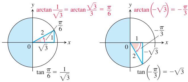
| x | arctan x |
| 1 | |
| 0 | 0 |
| -1 | |
The angles come from the first and fourth quadrants because the range of
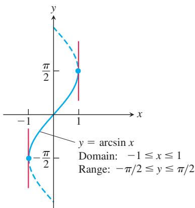
FIGURE 3.43 The graph of
The Derivative of 𝑦 = a r c s i n 𝑢
We know that the function
We find the derivative of
For
If
EXAMPLE 2 Using the Chain Rule, we calculate the derivative
The Derivative of 𝑦 = a r c t a n 𝑢
We find the derivative of
The derivative is defined for all real numbers:
The derivative is defined for all real numbers. If
The Chain Rule can also be combined with the arctangent function in other ways, as illustrated by the following example.
EXAMPLE 3
The Derivative of
Theorem 3 does not apply to the function
To express the result in terms of x, we use the relationships
to get
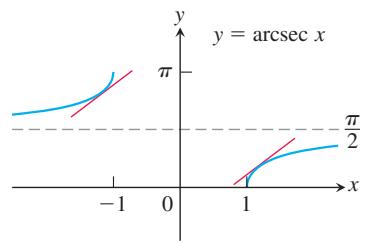
FIGURE 3.44 The slope of the curve
Can we do anything about the
With the absolute value symbol, we can write a single expression that eliminates the “±” ambiguity:
If u is a differentiable function of x with
EXAMPLE 4 Using the Chain Rule and derivative of the arcsecant function, we find
Derivatives of the Other Three Inverse Trigonometric Functions
We could use the same techniques to find the derivatives of the other three inverse trigonometric functions—arccosine, arccotangent, and arccosecant—but there is an easier way, thanks to the following identities.
Inverse Function–Inverse Cofunction Identities
We saw the first of these identities in Equation (5) of Section 1.5. The others are derived in a similar way. It follows easily that the derivatives of the inverse cofunctions are the negatives of the derivatives of the corresponding inverse functions. For example, the derivative of
The derivatives of the inverse trigonometric functions are summarized in Table 3.1.
TABLE 3.1 Derivatives of the inverse trigonometric functions
EXERCISES 3.9
Remember that arcsin and
Common Values
Use reference triangles in an appropriate quadrant, as in Example 1, to find the angles in Exercises 1–8.
-
a. arctan 1 b. arctan
( − √ 3 ) − 1 ( 1 √ 3 ) -
a. arctan
( − 1 ) − 1 √ 3 ( − 1 √ 3 ) -
a. arcsin
( − 1 2 ) ( 1 √ 2 ) − 1 ( − √ 3 2 ) -
a. sin
− 1 ( 1 2 ) ( − 1 √ 2 ) ( √ 3 2 ) -
a. arccos
( 1 2 ) − 1 ( − 1 √ 2 ) ( √ 3 2 ) -
a. csc
− 1 √ 2 ( − 2 √ 3 ) -
a.
s e c − 1 ( − √ 2 ) a r c s e c ( 2 √ 3 ) a r c s e c ( − 2 ) -
a.
a r c c o t ( − 1 ) a r c c o t ( √ 3 ) c o t − 1 ( − 1 √ 3 )
Evaluations
Find the values in Exercises 9–12.
9.
-
s e c ( a r c c o s 1 2 ) -
t a n ( a r c s i n ( − 1 2 ) ) -
c o t ( s i n − 1 ( − √ 3 2 ) )
Limits
Find the limits in Exercises 13–20. (If in doubt, look at the function’s graph.)
13.
-
l i m 𝑥 → − 1 + c o s − 1 𝑥 -
l i m 𝑥 → ∞ t a n − 1 𝑥 -
l i m 𝑥 → − ∞ a r c t a n 𝑥 -
l i m 𝑥 → ∞ a r c s e c 𝑥 -
l i m 𝑥 → − ∞ s e c − 1 𝑥 -
l i m 𝑥 → ∞ c s c − 1 𝑥 -
l i m 𝑥 → − ∞ a r c c s c 𝑥
Finding Derivatives
In Exercises 21–48, find the derivative of y with respect to the appropriate variable.
-
𝑦 = c o s − 1 ( 𝑥 2 ) -
𝑦 = a r c c o s ( 1 / 𝑥 ) -
𝑦 = a r c s i n √ 2 𝑡 -
𝑦 = s i n − 1 ( 1 − 𝑡 ) -
𝑦 = a r c s e c ( 2 𝑠 + 1 ) -
𝑦 = s e c − 1 5 𝑠 -
𝑦 = c s c − 1 ( 𝑥 2 + 1 ) , 𝑥 > 0 -
𝑦 = a r c c s c 𝑥 2 -
𝑦 = s e c − 1 1 𝑡 , 0 < 𝑡 < 1 -
𝑦 = a r c s i n 3 𝑡 2 -
𝑦 = a r c c o t √ 𝑡 -
𝑦 = c o t − 1 √ 𝑡 − 1 -
𝑦 = l n ( t a n − 1 𝑥 ) -
𝑦 = t a n − 1 ( l n 𝑥 ) -
𝑦 = a r c c s c ( 𝑒 𝑡 ) -
𝑦 = a r c c o s ( 𝑒 − 𝑡 ) -
𝑦 = 𝑠 √ 1 − 𝑠 2 + c o s − 1 𝑠 -
𝑦 = √ 𝑠 2 − 1 − s e c − 1 𝑠 -
𝑦 = t a n − 1 √ 𝑥 2 − 1 + c s c − 1 𝑥 , 𝑥 > 1 -
𝑦 = c o t − 1 1 𝑥 − t a n − 1 𝑥 -
𝑦 = 𝑥 a r c s i n 𝑥 + √ 1 − 𝑥 2 -
𝑦 = l n ( 𝑥 2 + 4 ) − 𝑥 a r c t a n ( 𝑥 2 ) -
𝑦 = √ a r c s i n 𝑥 -
𝑦 = 𝑒 a r c s e c 𝑥 -
𝑦 = c o s ( 𝑥 − a r c c o s 𝑥 ) -
𝑦 = 𝑥 1 + a r c t a n 𝑥 -
𝑦 = ( a r c c o t ( 𝑥 3 ) ) 3 -
𝑦 = l o g 2 a r c c s c √ 𝑥
For problems 49–52 use implicit differentiation to find
-
3 arctan
𝑥 + a r c s i n 𝑦 = 𝜋 4 𝑃 ( 1 , − 1 ) -
a r c s i n ( 𝑥 + 𝑦 ) + a r c c o s ( 𝑥 − 𝑦 ) = 5 𝜋 6 ; 𝑃 ( 0 , 1 2 ) -
𝑦 c o s − 1 ( 𝑥 𝑦 ) = − 3 √ 2 4 𝜋 ; 𝑃 ( 1 2 , − √ 2 ) -
1 6 ( t a n − 1 3 𝑦 ) 2 + 9 ( t a n − 1 2 𝑥 ) 2 = 2 𝜋 2 ; 𝑃 ( √ 3 2 , 1 3 )
Theory and Examples
- You are sitting in a classroom next to the wall looking at the blackboard at the front of the room. The blackboard is 4 m long and starts 1 m from the wall you are sitting next to. Show that your viewing angle is
if you are x meters from the front wall.
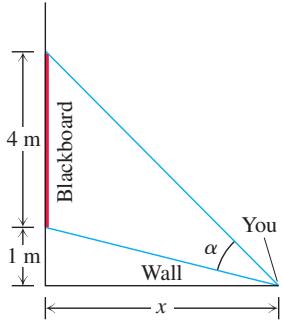
- Find the angle
𝛼
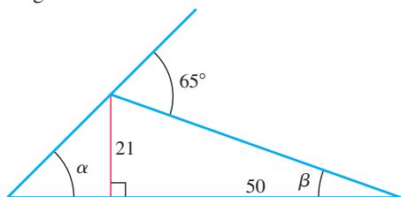
- Here is an informal proof that
t a n − 1 1 + t a n − 1 2 + t a n − 1 3 = 𝜋
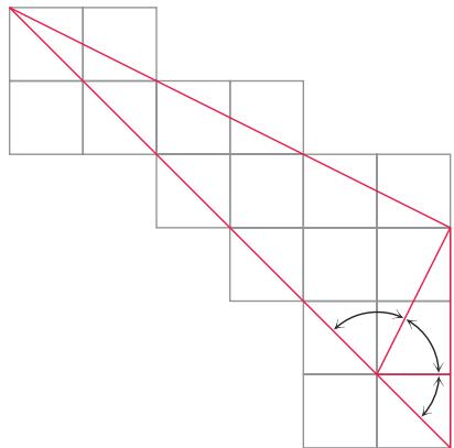
- Two derivations of the identity
s e c − 1 ( − 𝑥 ) = 𝜋 − s e c − 1 𝑥
a. (Geometric) Here is a pictorial proof that
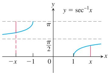
b. (Algebraic) Derive the identity
Which of the expressions in Exercises 57–60 are defined, and which are not? Give reasons for your answers.
- a. arctan 2
b.
-
a.
a r c c s c ( 1 / 2 ) -
a.
s e c − 1 0
b.
- a.
c o t − 1 ( − 1 / 2 )
b. arcsin
b.
- Use the identity
to derive the formula for the derivative of
- Derive the formula
for the derivative of
- Use the Derivative Rule in Section 3.8, Theorem 3, to derive
to derive the formula for the derivative of
- What is special about the functions
Explain.
- What is special about the functions
Explain.
T 67. Find the values of
T 68. Find the values of a.
In Exercises 69–71, find the domain and range of each composite function. Then graph the composition of the two functions on separate screens. Do the graphs make sense in each case? Give reasons for your answers. Comment on any differences you see.
-
a.
𝑦 = a r c t a n ( t a n 𝑥 ) 𝑦 = t a n ( a r c t a n 𝑥 ) -
a.
𝑦 = a r c s i n ( s i n 𝑥 ) 𝑦 = s i n ( a r c s i n 𝑥 ) -
a.
𝑦 = a r c c o s ( c o s 𝑥 ) 𝑦 = c o s ( a r c c o s 𝑥 )
T Use your graphing utility for Exercises 72–76.
-
Graph
𝑦 = s e c ( s e c − 1 𝑥 ) = s e c ( c o s − 1 ( 1 / 𝑥 ) ) -
Newton’s serpentine Graph Newton’s serpentine,
𝑦 = 4 𝑥 / ( 𝑥 2 + 1 ) 𝑦 = 2 s i n ( 2 t a n − 1 𝑥 ) -
Graph the rational function
𝑦 = ( 2 − 𝑥 2 ) / 𝑥 2 𝑦 = c o s ( 2 s e c − 1 𝑥 ) -
Graph
𝑓 ( 𝑥 ) = a r c s i n 𝑥 𝑓 ′ 𝑓 ″ -
Graph
𝑓 ( 𝑥 ) = a r c t a n 𝑥 𝑓 ′ 𝑓 ″
3.10 Related Rates
In this section we look at questions that arise when two or more related quantities are changing. The problem of determining how the rate of change of one of them affects the rates of change of the others is called a related rates problem.
Related Rates Equations
Suppose we are pumping air into a spherical balloon. Both the volume and radius of the balloon are increasing over time. If V is the volume and r is the radius of the balloon at an instant of time, then
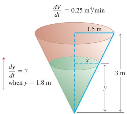
FIGURE 3.45 The geometry of the conical tank and the rate at which water fills the tank determine how fast the water level rises (Example 1).
Using the Chain Rule, we differentiate both sides with respect to t to find an equation relating the rates of change of V and r,
So if we know the radius r of the balloon and the rate dV/dt at which the volume is increasing at a given instant of time, then we can solve this last equation for dr/dt to find how fast the radius is increasing at that instant. Note that it is easier to directly measure the rate of increase of the volume (the rate at which air is being pumped into the balloon) than it is to measure the increase in the radius. The related rates equation allows us to calculate dr/dt from dV/dt.
Very often the key to relating the variables in a related rates problem is drawing a picture that shows the geometric relations between them, as illustrated in the following example.
EXAMPLE 1 Water runs into a conical tank at the rate of
Solution Figure 3.45 shows a partially filled conical tank. The variables in the problem are
x = radius (m) of the surface of the water at time t
We assume that
The water forms a cone with volume
This equation involves x as well as V and y. Because no information is given about x and dx/dt at the time in question, we need to eliminate x. The similar triangles in Figure 3.45 give us a way to express x in terms y:
Therefore, we find
to give the derivative
Finally, use y = 1.8 and dV/dt = 0.25 to solve for dy/dt.
At the moment in question, the water level is rising at about 0.098 m/min.
Related Rates Problem Strategy
-
Let t denote time, and choose names for all of the variables that change over time (we will assume that those variables are differentiable functions of t). Identify any quantities that remain constant (these do not need to be given names). In most problems it will be very helpful to draw a picture that depicts the setup of the problem.
-
Write an equation that relates the variables (and any constants that are present). You may have to combine two or more equations to get a single equation that relates the variable whose rate you want to the variables whose rates or values you know.
-
Differentiate with respect to t to obtain a related rates equation.
-
Substitute all of the numerical values provided in the problem into the related rates equation. You may need to use the equation(s) relating the variables (which you obtained in Step 2), or use other relationships (such as trigonometric identities), until you reach the point at which the only remaining unknown quantity is the rate of change that you are asked to find. Solve for this unknown.
EXAMPLE 2 A hot air balloon rising straight up from a level field is tracked by a range finder
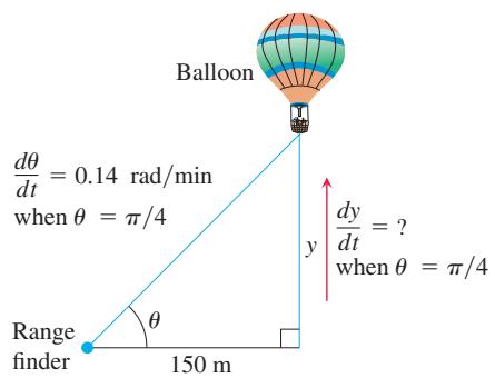
FIGURE 3.46 The rate of change of the balloon’s height is related to the rate of change of the angle the range finder makes with the ground (Example 2).
Solution We draw a picture (Figure 3.46) and name the variables that appear in the problem (which we assume are differentiable functions of t, where time is measured in minutes):
y = the height in meters of the balloon above the ground.
One constant in the picture is the distance from the range finder to the liftoff point (150m). There is no need to give this distance a special symbol.
FIGURE 3.47 The speed of the car is related to the speed of the police cruiser and the rate of change of the distance s between them (Example 3).
Trigonometry (Section 1.3) yields
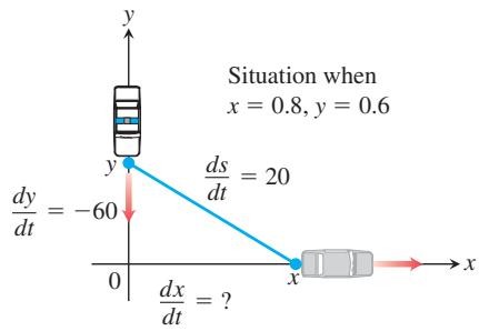
Equation relating the variables
By differentiating with respect to t using the Chain Rule, we obtain
Related rates equation
Substituting the known values
Thus, at the moment in question, the balloon is rising at the rate of 42 m/min.
EXAMPLE 3 A police cruiser, approaching a right-angled intersection from the north, is chasing a speeding car that has turned the corner and is now moving straight east. When the cruiser is 0.6 km north of the intersection and the car is 0.8 km to the east, the police determine with radar that the distance between them and the car is increasing at 30 km/h. If the cruiser is moving at 100 km/h at the instant of measurement, what is the speed of the car?
Solution We picture the car and cruiser in the coordinate plane, using the positive x-axis as the eastbound highway and the positive y-axis as the southbound highway (Figure 3.47). We let t represent time and set
s = distance between car and cruiser at time t
We assume that x, y, and s are differentiable functions of t.
We want to find
Note that dy/dt is negative because y is decreasing.
We differentiate the distance equation between the car and the cruiser,
(we could also use
Finally, we use
At the moment in question, the car’s speed is
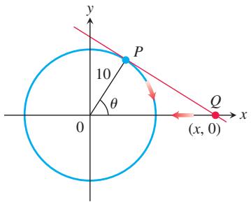
FIGURE 3.48 The particle P travels clockwise along the circle (Example 4).
EXAMPLE 4 A particle
Solution We picture the situation in the coordinate plane with the circle centered at the origin (see Figure 3.48). We let t represent time and let
Setting
Equation relating the variables
Differentiation with respect to t gives
We want to find
Note that
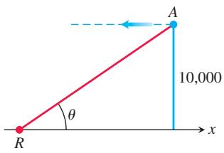
EXAMPLE 5 A jet airliner is flying at a constant altitude of 10,000 m above sea level as it approaches a Pacific island. The aircraft comes within the direct line of sight of a radar station located on the island, and the radar indicates the initial angle between sea level and its line of sight to the aircraft is
FIGURE 3.49 Jet airliner A traveling at constant altitude toward radar station R (Example 5).
Solution The aircraft A and radar station R are pictured in the coordinate plane, using the positive x-axis as the horizontal distance at sea level from R to A, and the positive y-axis as the vertical altitude above sea level. We let t represent time and observe that y = 10,000 is a constant. The general situation and line-of-sight angle
From Figure 3.49, we see that
Using kilometers instead of meters for our distance units, the last equation translates to
Differentiation with respect to t gives
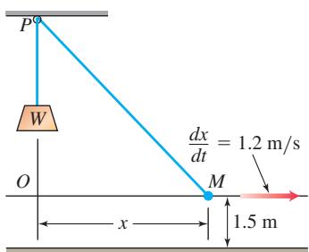
(a)
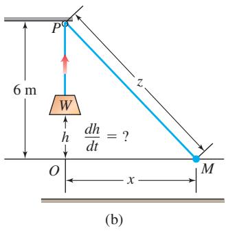
FIGURE 3.50 A worker at M walks to the right, pulling the weight W upward as the rope moves through the pulley P (Example 6).
When
Substitution into the equation for dx/dt then gives
The negative sign appears because the distance x is decreasing, so the aircraft is approaching the island at a speed of approximately 838 km/h when first detected by the radar.
Note that the solution of Example 5 involved several unit conversions: from seconds to hours and from degrees to radians. When solving related rates problems, we should check that consistent units are used.
EXAMPLE 6 Figure 3.50a shows a rope running through a pulley at P and bearing a weight W at one end. The other end is held 1.5 m above the ground in the hand M of a worker. Suppose the pulley is 7.5 m above ground, the rope is 13.5 m long, and the worker is walking rapidly away from the vertical line PW at the rate of 1.2 m/s. How fast is the weight being raised when the worker’s hand is 6.3 m away from PW?
Solution We let
At any instant of time t, we have the following relationships (see Figure 3.50b):
If we solve for
Differentiating both sides with respect to t gives
and solving this last equation for dh/dt we find
Since we know
so that
Equation (2) now gives
as the rate at which the weight is being raised when
EXERCISES 3.10
-
Area Suppose that the radius
𝑟 𝐴 = 𝜋 𝑟 2 𝑡 𝑑 𝐴 / 𝑑 𝑡 𝑑 𝑟 / 𝑑 𝑡 -
Surface area Suppose that the radius r and surface area
𝑆 = 4 𝜋 𝑟 2 -
Assume that
𝑦 = 5 𝑥 𝑑 𝑥 / 𝑑 𝑡 = 2 𝑑 𝑦 / 𝑑 𝑡 -
Assume that
2 𝑥 + 3 𝑦 = 1 2 -
If
𝑦 = 𝑥 2 𝑑 𝑥 / 𝑑 𝑡 = 3 𝑑 𝑦 / 𝑑 𝑡 𝑥 = − 1 -
If
𝑥 = 𝑦 3 − 𝑦 -
If
𝑥 2 + 𝑦 2 = 2 5 𝑑 𝑥 / 𝑑 𝑡 = − 2 𝑑 𝑦 / 𝑑 𝑡 𝑥 = 3 𝑦 = − 4 -
If
𝑥 2 𝑦 3 = 4 / 2 7 -
If
𝐿 = √ 𝑥 2 + 𝑦 2 𝑑 𝑥 / 𝑑 𝑡 = − 1 𝑑 𝑦 / 𝑑 𝑡 = 3 𝑑 𝐿 / 𝑑 𝑡 𝑥 = 5 𝑦 = 1 2 -
If
𝑟 + 𝑠 2 + 𝑣 3 = 1 2 -
If the original 24 m edge length x of a cube decreases at the rate of 5 m/min, when x = 3 m at what rate does the cube’s a. surface area change? b. volume change?
-
A cube’s surface area increases at the rate of
7 2 c m 2 / s 𝑥 = 3 c m -
Volume The radius
𝑟 ℎ 𝑉 𝑉 = 𝜋 𝑟 2 ℎ
a. How is
b. How is
c. How is
- Volume The radius
𝑟 ℎ 𝑉 𝑉 = ( 1 / 3 ) 𝜋 𝑟 2 ℎ
a. How is
b. How is
c. How is
- Changing voltage The voltage V (volts), current I (amperes), and resistance R (ohms) of an electric circuit like the one shown here are related by the equation V = IR. Suppose that V is increasing at the rate of 1 volt/s while I is decreasing at the rate of 1/3 amp/s. Let t denote time in seconds.
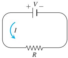
a. What is the value of
b. What is the value of
c. What equation relates
d. Find the rate at which R is changing when V = 12 volts and I = 2 amps. Is R increasing, or decreasing?
- Electrical power The power
𝑃 𝑅 𝐼 𝑃 = 𝑅 𝐼 2
a. How are
b. How is
- Distance Let
𝑥 𝑦 𝑡 𝑠 = √ 𝑥 2 + 𝑦 2 ( 𝑥 , 0 ) ( 0 , 𝑦 ) 𝑥 𝑦
a. How is ds/dt related to dx/dt if y is constant?
b. How is ds/dt related to dx/dt and dy/dt if neither x nor y is constant?
c. How is
- Diagonals If
𝑥 , 𝑦 𝑧 𝑠 = √ 𝑥 2 + 𝑦 2 + 𝑧 2
a. Assuming that
b. How is ds/dt related to dy/dt and dz/dt if x is constant?
c. How are
- Area The area A of a triangle with sides of lengths a and b enclosing an angle of measure
𝜃
a. How is dA/dt related to
b. How is dA/dt related to
c. How is
-
Heating a plate When a circular plate of metal is heated in an oven, its radius increases at the rate of
0 . 0 1 c m / m i n 5 0 c m -
Changing dimensions in a rectangle The length l of a rectangle is decreasing at the rate of 2 cm/s while the width w is increasing at the rate of 2 cm/s. When l = 12 cm and w = 5 cm, find the rates of change of (a) the area, (b) the perimeter, and (c) the lengths of the diagonals of the rectangle. Which of these quantities are decreasing, and which are increasing?
-
Changing dimensions in a rectangular box Suppose that the edge lengths x, y, and z of a closed rectangular box are changing at the following rates:
Find the rates at which the box’s (a) volume, (b) surface area, and (c) diagonal length
- A sliding ladder A 3.9-m ladder is leaning against a house when its base starts to slide away (see accompanying figure). By the time the base is 3.6 m from the house, the base is moving at the rate of 1.5 m/s.
a. How fast is the top of the ladder sliding down the wall then?
b. At what rate is the area of the triangle formed by the ladder, wall, and ground changing then?
c. At what rate is the angle
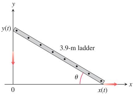
-
Commercial air traffic Two commercial airplanes are flying at an altitude of 12,000 m along straight-line courses that intersect at right angles. Plane A is approaching the intersection point at a speed of 442 knots (nautical miles per hour; a nautical mile is 1852 m). Plane B is approaching the intersection at 481 knots. At what rate is the distance between the planes changing when A is 5 nautical miles from the intersection point, and B is 12 nautical miles from the intersection point?
-
Flying a kite A girl flies a kite at a height of 90 m, the wind carrying the kite horizontally away from her at a rate of 7.5 m/s. How fast must she let out the string when the kite is 150 m away from her?
-
Boring a cylinder The mechanics at Lincoln Automotive are reboring a 15-cm-deep cylinder to fit a new piston. The machine they are using increases the cylinder’s radius one-thousandth of a centimeter every 3 min. How rapidly is the cylinder volume increasing when the bore (diameter) is 10 cm?
-
A growing sand pile Sand falls from a conveyor belt at the rate of
1 0 𝑚 3 / 𝑚 𝑖 𝑛 -
A draining conical reservoir Water is flowing at the rate of
5 0 𝑚 3 / 𝑚 𝑖 𝑛
a. How fast (in centimeters per minute) is the water level falling when the water is 5 m deep?
b. How fast is the radius of the water’s surface changing then? Answer in centimeters per minute.
- A draining hemispherical reservoir Water is flowing at the rate of
6 𝑚 3 / 𝑚 𝑖 𝑛 𝑉 = ( 𝜋 / 3 ) 𝑦 2 ( 3 𝑅 − 𝑦 )
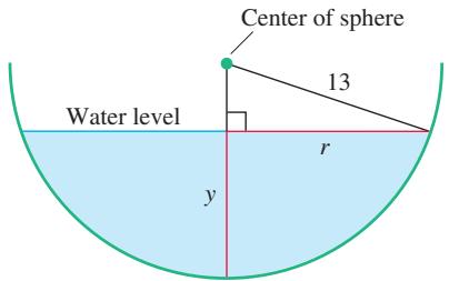
a. At what rate is the water level changing when the water is 8 m deep?
b. What is the radius
c. At what rate is the radius r changing when the water is 8 m deep?
-
A growing raindrop Suppose that a drop of mist is a perfect sphere and that, through condensation, the drop picks up moisture at a rate proportional to its surface area. Show that under these circumstances the drop’s radius increases at a constant rate.
-
The radius of an inflating balloon A spherical balloon is inflated with helium at the rate of
1 0 0 𝜋 m 3 / m i n 5 m -
Hauling in a dinghy A dinghy is pulled toward a dock by a rope from the bow through a ring on the dock 2 m above the bow. The rope is hauled in at the rate of 0.5 m/s.
a. How fast is the boat approaching the dock when 3 m of rope are out?
b. At what rate is the angle
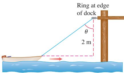
- A balloon and a bicycle A balloon is rising vertically above a level, straight road at a constant rate of 0.3 m/s. Just when the balloon is 20 m above the ground, a bicycle moving at a constant rate of 5 m/s passes under it. How fast is the distance
𝑠 ( 𝑡 )
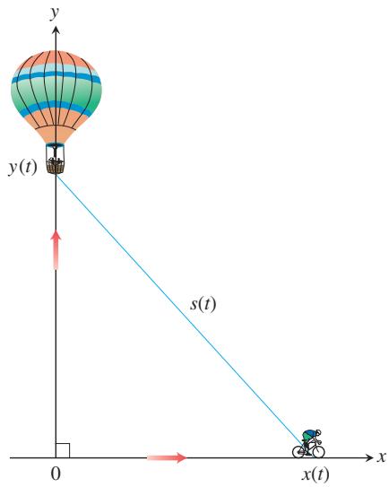
- Making coffee Coffee is draining from a conical filter into a cylindrical coffeepot at the rate of
1 6 0 c m 3 / m i n
a. How fast is the level in the pot rising when the coffee in the cone is 12 cm deep?
b. How fast is the level in the cone falling then?
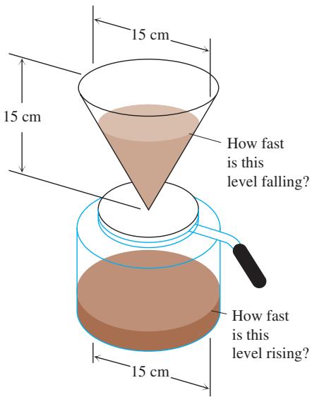
- Cardiac output In the late 1860s, Adolf Fick, a professor of physiology in the Faculty of Medicine in Würzberg, Germany, developed one of the methods we use today for measuring how much blood your heart pumps in a minute. Your cardiac output as you read this sentence is probably about 7 L/min. At rest it is likely to be a bit under 6 L/min. If you are a trained marathon runner running a marathon, your cardiac output can be as high as 30 L/min.
Your cardiac output can be calculated with the formula
where Q is the number of milliliters of
fairly close to the 6 L/min that most people have at basal (resting) conditions. (Data courtesy of J. Kenneth Herd, M.D., Quillan College of Medicine, East Tennessee State University.)
Suppose that when Q = 233 and D = 41, we also know that D is decreasing at the rate of 2 units a minute but that Q remains unchanged. What is happening to the cardiac output?
-
Moving along a parabola A particle moves along the parabola
𝑦 = 𝑥 2 𝜃 -
Motion in the plane The coordinates of a particle in the metric xy-plane are differentiable functions of time t with dx/dt = -1 m/s and dy/dt = -5 m/s. How fast is the particle’s distance from the origin changing as it passes through the point
( 5 , 1 2 ) -
Videotaping a moving car You are videotaping a race from a stand 40 m from the track, following a car that is moving at 288 km/h (80 m/s), as shown in the accompanying figure. How fast will your camera angle
𝜃
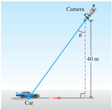
- A moving shadow A light shines from the top of a pole
1 5 m 9 m 1 / 2 s 𝑠 = 4 . 9 𝑡 2 m 𝑡
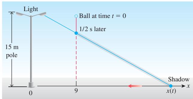
- A building’s shadow On a morning of a day when the sun will pass directly overhead, the shadow of a 24 m building on level ground is 18 m long. At the moment in question, the angle
𝜃 0 . 2 7 ∘ / m i n
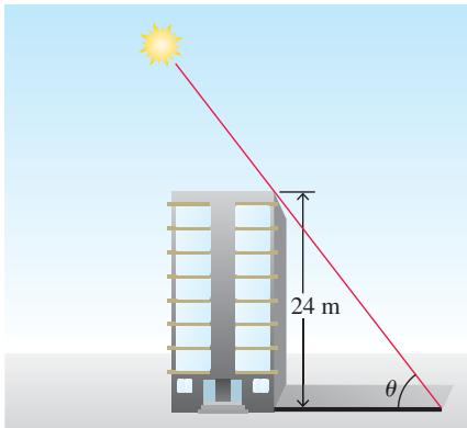
-
A melting ice layer A spherical iron ball 8 cm in diameter is coated with a layer of ice of uniform thickness. If the ice melts at the rate of
1 0 𝑐 𝑚 3 / 𝑚 𝑖 𝑛 -
Highway patrol A highway patrol plane flies
3 k m 1 2 0 k m / h 5 k m 1 6 0 k m / h -
Baseball players A baseball diamond is a square 27 m on a side. A player runs from first base to second at a rate of 5 m/s.
a. At what rate is the player’s distance from third base changing when the player is
b. At what rates are angles
c. The player slides into second base at the rate of 4.5 m/s. At what rates are angles
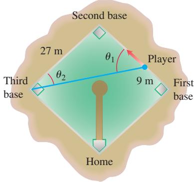
-
Ships Two ships are steaming straight away from a point O along routes that make a
1 2 0 ∘ -
Clock’s moving hands At what rate is the angle between a clock’s minute and hour hands changing at 4 o’clock in the afternoon?
-
Oil spill An explosion at an oil rig located in gulf waters causes an elliptical oil slick to spread on the surface from the rig. The slick is a constant 20 cm thick. After several days, when the major axis of the slick is 2 km long and the minor axis is 3/4 km wide, it is determined that its length is increasing at the rate of 9 m/h, and its width is increasing at the rate of 3 m/h. At what rate (in cubic meters per hour) is oil flowing from the site of the rig at that time?
-
A lighthouse beam A lighthouse sits 1 km offshore, and its beam of light rotates counterclockwise at the constant rate of 3 full circles per minute. At what rate is the image of the beam moving down the shoreline when the image is 1 km from the spot on the shoreline nearest the lighthouse?
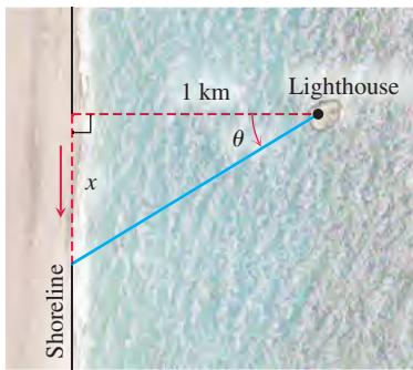
3.11 Linearization and Differentials
It is often useful to approximate complicated functions with simpler ones that give the accuracy we want for specific applications and, at the same time, are easier to work with than the original functions. The approximating functions discussed in this section are called linearizations, and they are based on tangent lines. Other approximating functions, such as polynomials, are discussed in Chapter 9.
We introduce new variables
Linearization
As you can see in Figure 3.51, the tangent line to the curve
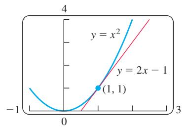
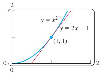
Tangent line and curve very close near
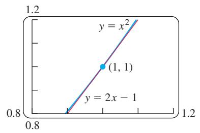
Tangent line and curve very close throughout entire x-interval shown.
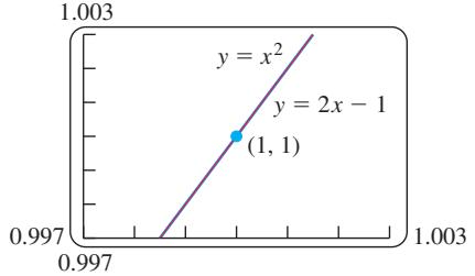
Tangent line and curve closer still. Computer screen cannot distinguish tangent line from curve on this x-interval.
FIGURE 3.51 The more we magnify the graph of a function near a point where the function is differentiable, the flatter the graph becomes and the more it resembles its tangent line.
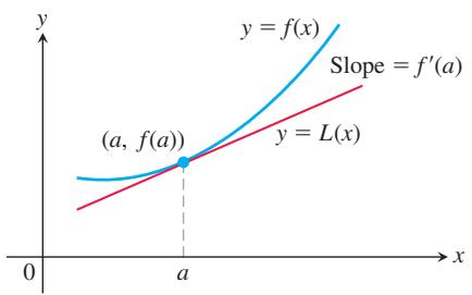
FIGURE 3.52 The tangent line to the curve
In general, the tangent line to
Thus, this tangent line is the graph of the linear function
As long as this line remains close to the graph of f as we move off the point of tangency,
DEFINITIONS If f is differentiable at x = a, then the approximating function
𝐿 ( 𝑥 ) = 𝑓 ( 𝑎 ) + 𝑓 ′ ( 𝑎 ) ( 𝑥 − 𝑎 ) is the linearization of f at a. The approximation
𝑓 ( 𝑥 ) ≈ 𝐿 ( 𝑥 )
of f by L is the standard linear approximation of f at a. The point x = a is the center of the approximation.
EXAMPLE 1 Find the linearization of
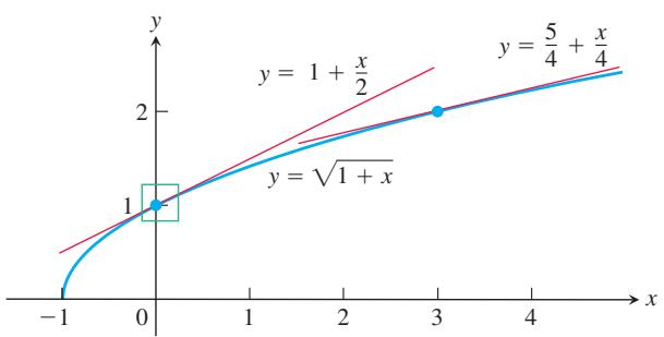
FIGURE 3.53 The graph of
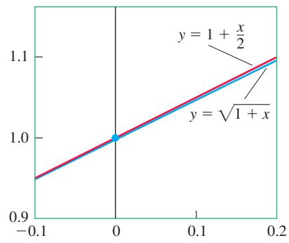
FIGURE 3.54 Magnified view of the window in Figure 3.53.
Solution Since
we have
See Figure 3.54.
The following table shows how accurate the approximation
| Approximation | True value | |True value - approximation| |
| 1.002497 | ||
| 1.024695 | ||
| 1.095445 |
Do not be misled by the preceding calculations into thinking that whatever we do with a linearization is better done with a calculator. In practice, we would never use a linearization to find a particular square root. The utility of a linearization is its ability to replace a complicated formula by a simpler one over an entire interval of values. If we have to work with
A linear approximation normally loses accuracy away from its center. As Figure 3.53 suggests, the approximation
EXAMPLE 2 Find the linearization of
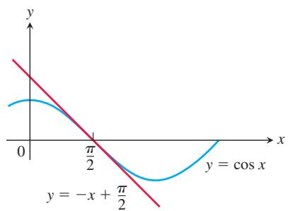
FIGURE 3.55 The graph of
we have
Approximations Near
Solution We evaluate the equation defining
At
which differs from the true value
a result that is off by more than 25%.
EXAMPLE 3 Find the linearization of
Solution Since
An important linear approximation for roots and powers is
(Exercise 15). This approximation, which is good for values of x sufficiently close to zero, has broad application. For example, when x is small,
Differentials
We sometimes use the Leibniz notation dy/dx to represent the derivative of y with respect to x. Contrary to its appearance, it is not a ratio. We now introduce two new variables dx and dy with the property that when their ratio exists, it is equal to the derivative.
DEFINITION Let
be a differentiable function. The differential dx is an independent variable. The differential dy is 𝑦 = 𝑓 ( 𝑥 ) 𝑑 𝑦 = 𝑓 ′ ( 𝑥 ) 𝑑 𝑥 .
Unlike the independent variable dx, the variable dy is always a dependent variable. It depends on both x and dx. If dx is given a specific value and x is a particular number in the domain of the function f, then these values determine the numerical value of dy. Often the variable dx is chosen to be
EXAMPLE 4
(a) Find dy if
(b) Find the value of dy when x = 1 and dx = 0.2.
Solution
(a)
(b) Substituting x = 1 and dx = 0.2 in the expression for dy, we have
The geometric meaning of differentials is shown in Figure 3.56. Let
The corresponding change in the tangent line L is
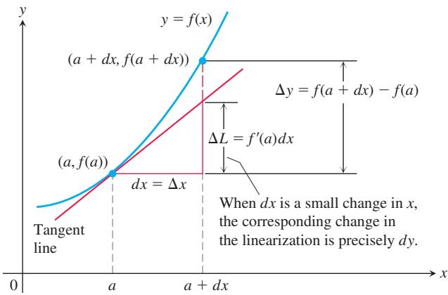
FIGURE 3.56 Geometrically, the differential dy is the change
That is, the change in the linearization of f is precisely the value of the differential dy when x = a and dx =
If
We sometimes write
in place of
Every differentiation formula like
has a corresponding differential form like
EXAMPLE 5 We can use the Chain Rule and other differentiation rules to find differentials of functions.
Estimating with Differentials
Suppose we know the value of a differentiable function
FIGURE 3.57 When dr is small compared with a, the differential dA gives the estimate
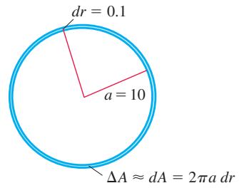
the differential approximation gives
when
EXAMPLE 6 The radius
Solution Since
Thus, since
The area of a circle of radius 10.1 m is approximately
The true area is
The error in our estimate is
When using differentials to estimate functions, our goal is to choose a nearby point x = a where both
EXAMPLE 7 Use differentials to estimate
Solution
(a) The differential associated with the cube root function
We set
This gives an approximation to the true value of
(b) The differential associated with
To estimate
For comparison, the true value of
The method in part (b) of Example 7 can be used in computer algorithms to give values of trigonometric functions. The algorithms store a large table of sine and cosine values between 0 and
Error in Differential Approximation
Let
The true change:
The differential estimate:
How well does
We measure the approximation error by subtracting df from
As
approaches
Although we do not know the exact size of the error, it is the product
Change in
in which
In Example 6 we found that
so the approximation error is
Proof of the Chain Rule
Equation (1) enables us to give a complete proof of the Chain Rule. Our goal is to show that if
Let
where
where
SO
Since
Sensitivity to Change
The equation
| True | Estimated | |
| Absolute change | ||
| Relative change | ||
| Percentage change |
EXAMPLE 8 You want to calculate the depth of a well from the equation
Solution The size of ds in the equation
depends on how big t is. If t = 2 s, the change caused by dt = 0.1 is about
Three seconds later at t = 5 s, the change caused by the same dt is
For a fixed error in the time measurement, the error in using ds to estimate the depth is larger when it takes a longer time before the stone splashes into the water. That is, the estimate is more sensitive to the effect of the error for larger values of t.
EXAMPLE 9 Newton’s second law,
is stated with the assumption that mass is constant, but we know this is not strictly true because the mass of an object increases with velocity. In Einstein’s corrected formula, mass has the value
where the “rest mass”
to estimate the increase
Solution When
to obtain
or
Equation (3) expresses the increase in mass that results from the added velocity v.
Converting Mass to Energy
Equation (3) derived in Example 9 has an important interpretation. In Newtonian physics,
we see that
or
So the change in kinetic energy
Exercises 3.11
Finding Linearizations
In Exercises 1–5, find the linearization
Applications
-
𝑓 ( 𝑥 ) = 𝑥 3 − 2 𝑥 + 3 , 𝑎 = 2 -
𝑓 ( 𝑥 ) = √ 𝑥 2 + 9 , 𝑎 = − 4 -
𝑓 ( 𝑥 ) = 𝑥 + 1 𝑥 , 𝑎 = 1 -
𝑓 ( 𝑥 ) = 3 √ 𝑥 , 𝑎 = − 8 -
𝑓 ( 𝑥 ) = t a n 𝑥 , 𝑎 = 𝜋 -
Common linear approximations at
𝑥 = 0 𝑥 = 0
a.
Linearization for Approximation
In Exercises 7–14, find a linearization at a suitably chosen integer near
-
𝑓 ( 𝑥 ) = 𝑥 2 + 2 𝑥 , 𝑎 = 0 . 1 -
𝑓 ( 𝑥 ) = 𝑥 − 1 𝑎 = 0 . 9 -
𝑓 ( 𝑥 ) = 2 𝑥 2 + 3 𝑥 − 3 , 𝑎 = − 0 . 9 -
𝑓 ( 𝑥 ) = 1 + 𝑥 , 𝑎 = 8 . 1 -
𝑓 ( 𝑥 ) = 3 √ 𝑥 , 𝑎 = 8 . 5 -
𝑓 ( 𝑥 ) = 𝑥 𝑥 + 1 , 𝑎 = 1 . 3 -
𝑓 ( 𝑥 ) = 𝑒 − 𝑥 𝑎 = − 0 . 1 -
𝑓 ( 𝑥 ) = s i n − 1 𝑥 , 𝑎 = 𝜋 / 1 2 -
Show that the linearization of
𝑓 ( 𝑥 ) = ( 1 + 𝑥 ) 𝑘 𝑥 = 0 𝐿 ( 𝑥 ) = 1 + 𝑘 𝑥 -
Use the linear approximation
( 1 + 𝑥 ) 𝑘 ≈ 1 + 𝑘 𝑥 𝑓 ( 𝑥 ) 𝑓 ( 𝑥 ) = ( 1 − 𝑥 ) 6 𝑓 ( 𝑥 ) = 2 1 − 𝑥 𝑓 ( 𝑥 ) = 1 √ 1 + 𝑥 𝑓 ( 𝑥 ) = √ 2 + 𝑥 2 𝑓 ( 𝑥 ) = ( 4 + 3 𝑥 ) 1 / 3 𝑓 ( 𝑥 ) = 3 √ ( 1 − 𝑥 2 + 𝑥 ) 2 -
Faster than a calculator Use the approximation
( 1 + 𝑥 ) 𝑘 ≈ 1 + 𝑘 𝑥 ( 1 . 0 0 0 2 ) 5 0 3 √ 1 . 0 0 9 -
Find the linearization of
𝑓 ( 𝑥 ) = √ 𝑥 + 1 + s i n 𝑥 √ 𝑥 + 1 s i n 𝑥
Derivatives in Differential Form
In Exercises 19–38, find dy.
-
𝑦 = 𝑥 3 − 3 √ 𝑥 -
𝑦 = 𝑥 √ 1 − 𝑥 2 -
𝑦 = 2 𝑥 1 + 𝑥 2 -
𝑦 = 2 √ 𝑥 3 ( 1 + √ 𝑥 ) -
2 𝑦 3 / 2 + 𝑥 𝑦 − 𝑥 = 0 -
𝑥 𝑦 2 − 4 𝑥 3 / 2 − 𝑦 = 0 -
𝑦 = s i n ( 5 √ 𝑥 ) -
𝑦 = c o s ( 𝑥 2 ) -
𝑦 = 4 t a n ( 𝑥 3 / 3 ) -
𝑦 = s e c ( 𝑥 2 − 1 ) -
𝑦 = 3 c s c ( 1 − 2 √ 𝑥 ) -
𝑦 = 2 c o t ( 1 √ 𝑥 ) -
𝑦 = 𝑒 √ 𝑥 -
𝑦 = 𝑥 𝑒 − 𝑥 -
𝑦 = l n ( 1 + 𝑥 2 ) -
𝑦 = l n ( 𝑥 + 1 √ 𝑥 − 1 ) -
𝑦 = t a n − 1 ( 𝑒 𝑥 2 ) -
𝑦 = c o t − 1 ( 1 𝑥 2 ) + c o s − 1 2 𝑥 -
𝑦 = s e c − 1 ( 𝑒 − 𝑥 ) -
𝑦 = 𝑒 t a n − 1 √ 𝑥 2 + 1
Approximation Error
In Exercises 39–44, each function
a. the change
b. the value of the estimate
c. the approximation error
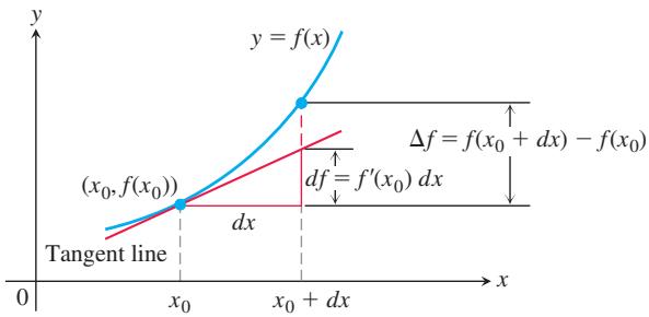
-
𝑓 ( 𝑥 ) = 𝑥 2 + 2 𝑥 , 𝑥 0 = 1 , 𝑑 𝑥 = 0 . 1 -
𝑓 ( 𝑥 ) = 2 𝑥 2 + 4 𝑥 − 3 , 𝑥 0 = − 1 , 𝑑 𝑥 = 0 . 1 -
𝑓 ( 𝑥 ) = 𝑥 3 − 𝑥 , 𝑥 0 = 1 , 𝑑 𝑥 = 0 . 1 -
𝑓 ( 𝑥 ) = 𝑥 4 𝑥 0 = 1 -
𝑓 ( 𝑥 ) = 𝑥 − 1 𝑥 0 = 0 . 5 𝑑 𝑥 = 0 . 1 -
𝑓 ( 𝑥 ) = 𝑥 3 − 2 𝑥 + 3 , 𝑥 0 = 2 , 𝑑 𝑥 = 0 . 1
Differential Estimates of Change
In Exercises 45–50, write a differential formula that estimates the given change in volume or surface area.
-
The change in the volume
𝑉 = ( 4 / 3 ) 𝜋 𝑟 3 𝑟 0 𝑟 0 + 𝑑 𝑟 -
The change in the volume
𝑉 = 𝑥 3 𝑥 0 𝑥 0 + 𝑑 𝑥 -
The change in the surface area
𝑆 = 6 𝑥 2 𝑥 0 𝑥 0 + 𝑑 𝑥 -
The change in the lateral surface area
𝑆 = 𝜋 𝑟 √ 𝑟 2 + ℎ 2 𝑟 0 𝑟 0 + 𝑑 𝑟 -
The change in the volume
𝑉 = 𝜋 𝑟 2 ℎ 𝑟 0 𝑟 0 + 𝑑 𝑟 -
The change in the lateral surface area
𝑆 = 2 𝜋 𝑟 ℎ ℎ 0 ℎ 0 + 𝑑 ℎ -
The radius of a circle is increased from 2.00 to 2.02 m.
a. Estimate the resulting change in area.
b. Express the estimate as a percentage of the circle’s original area.
-
The diameter of a tree was 25 cm. During the following year, the circumference increased 5 cm. About how much did the tree’s diameter increase? What is the tree’s cross-sectional area?
-
Estimating volume Estimate the volume of material in a cylindrical shell with length 30 cm, radius 6 cm, and shell thickness 0.5 cm.
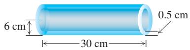
-
Estimating height of a building A surveyor, standing 9 m from the base of a building, measures the angle of elevation to the top of the building to be
7 5 ∘ -
The radius
𝑟 2 % -
The edge
𝑥 0 . 5 % -
Tolerance The height and radius of a right circular cylinder are equal, so the cylinder’s volume is
𝑉 = 𝜋 ℎ 3 -
Tolerance
a. About how accurately must the interior diameter of a 10-m-high cylindrical storage tank be measured to calculate the tank’s volume to within
b. About how accurately must the tank’s exterior diameter be measured to calculate the amount of paint it will take to paint the side of the tank to within
-
The diameter of a sphere is measured as
1 0 0 ± 1 -
Estimate the allowable percentage error in measuring the diameter D of a sphere if the volume is to be calculated correctly to within 3%.
-
The effect of flight maneuvers on the heart The amount of work done by the heart’s main pumping chamber, the left ventricle, is given by the equation
where W is the work per unit time, P is the average blood pressure, V is the volume of blood pumped out during the unit of time,
When
As a member of NASA’s medical team, you want to know how sensitive
- Drug concentration The concentration
𝐶 𝑡
Estimate the change in concentration when t changes from 20 to 30 min.
-
Unclogging arteries The formula
𝑉 = 𝑘 𝑟 4 -
Measuring acceleration of gravity When the length L of a clock pendulum is held constant by controlling its temperature, the pendulum’s period T depends on the acceleration of gravity g. The period will therefore vary slightly as the clock is moved from place to place on Earth’s surface, depending on the change in g. By keeping track of
Δ 𝑇 𝑇 = 2 𝜋 ( 𝐿 / 𝑔 ) 1 / 2
a. With L held constant and g as the independent variable, calculate dT and use it to answer parts (b) and (c).
b. If g increases, will T increase or decrease? Will a pendulum clock speed up or slow down? Explain.
T c. A clock with a 100-cm pendulum is moved from a location where
- Quadratic approximations
a. Let
i.
Determine the coefficients
b. Find the quadratic approximation to
T c. Graph
d. Find the quadratic approximation to
T e. Find the quadratic approximation to
x = 0. Graph h and its quadratic approximation together. Comment on what you see.
f. What are the linearizations of
- The linearization is the best linear approximation Suppose that
𝑦 = 𝑓 ( 𝑥 ) 𝑥 = 𝑎 𝑔 ( 𝑥 ) = 𝑔 ( 𝑥 ) = 𝑚 ( 𝑥 − 𝑎 ) + 𝑐 𝑚 𝑐 𝐸 ( 𝑥 ) = 𝑓 ( 𝑥 ) − 𝑔 ( 𝑥 ) 𝑥 = 𝑎 𝑔 𝑓 𝐿 ( 𝑥 ) = 𝑓 ( 𝑎 ) + 𝑓 ′ ( 𝑎 ) ( 𝑥 − 𝑎 ) 𝑔
-
𝐸 ( 𝑎 ) = 0 -
l i m 𝑥 → 𝑎 𝐸 ( 𝑥 ) 𝑥 − 𝑎 = 0
The approximation error is zero at x = a. The error is negligible when compared with x - a.
then
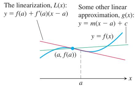
- The linearization of
2 𝑥
a. Find the linearization of
T b. Graph the linearization and function together for
- The linearization of
l o g 3 𝑥
a. Find the linearization of
T b. Graph the linearization and function together in the window
COMPUTER EXPLORATIONS
In Exercises 69–74, use a CAS to estimate the magnitude of the error in using the linearization in place of the function over a specified interval I. Perform the following steps:
a. Plot the function f over I.
b. Find the linearization L of the function at the point a.
c. Plot f and L together on a single graph.
d. Plot the absolute error
e. From your graph in part (d), estimate as large a
for
-
𝑓 ( 𝑥 ) = 𝑥 3 + 𝑥 2 − 2 𝑥 , [ − 1 , 2 ] , 𝑎 = 1 -
𝑓 ( 𝑥 ) = 𝑥 − 1 4 𝑥 2 + 1 , [ − 3 4 , 1 ] , 𝑎 = 1 2
CHAPTER 3 Questions to Guide Your Review
-
What is the derivative of a function
𝑓 𝑓 -
What role does the derivative play in defining slopes, tangent lines, and rates of change?
-
How can you sometimes graph the derivative of a function when all you have is a table of the function’s values?
-
What does it mean for a function to be differentiable on an open interval? On a closed interval?
-
How are derivatives and one-sided derivatives related?
-
Describe geometrically when a function typically does not have a derivative at a point.
-
What rules do you know for calculating derivatives? Give some examples.
-
How is a function’s differentiability at a point related to its continuity there, if at all?
-
Explain how the three formulas
a.
enable us to differentiate any polynomial.
-
What formula do we need, in addition to the three listed in Question 9, to differentiate rational functions?
-
What is a second derivative? A third derivative? How many derivatives do the functions you know have? Give examples.
-
What is the derivative of the exponential function
𝑒 𝑥 -
What is the relationship between a function’s average and instantaneous rates of change? Give an example.
-
How do derivatives arise in the study of motion? What can you learn about an object’s motion along a line by examining the derivatives of the object’s position function? Give examples.
-
How can derivatives arise in economics?
-
What is the derivative of
l o g 𝑎 𝑥 -
Give examples of still other applications of derivatives.
-
What do the limits
l i m ℎ → 0 ( ( s i n ℎ ) / ℎ ) l i m ℎ → 0 ( ( c o s ℎ − 1 ) / ℎ ) -
Once you know the derivatives of
s i n 𝑥 c o s 𝑥 t a n 𝑥 c o t 𝑥 s e c 𝑥 c s c 𝑥 -
What is the rule for calculating the derivative of a composition of two differentiable functions? How is such a derivative evaluated? Give examples.
-
If
𝑢 𝑥 ( 𝑑 / 𝑑 𝑥 ) ( 𝑢 𝑛 ) 𝑛 𝑛 -
What is logarithmic differentiation? Give an example.
-
How can you write any real power of
𝑥 𝑒 𝑥 -
What are the derivatives of the inverse trigonometric functions? How do the domains of the derivatives compare with the domains of the functions?
-
What is one way of expressing the special number
𝑒 𝑒 -
What is implicit differentiation? When do you need it? Give examples.
-
How do related rates problems arise? Give examples.
-
Outline a strategy for solving related rates problems. Illustrate with an example.
-
What is the derivative of the natural logarithm function
l n 𝑥 -
What is the linearization
𝐿 ( 𝑥 ) 𝑓 ( 𝑥 ) -
If x moves from a to a nearby value
𝑎 + 𝑑 𝑥 𝑓 ( 𝑥 ) -
What is the derivative of the exponential function
𝑎 𝑥 , 𝑎 > 0 𝑎 ≠ 1 ( 𝑎 ℎ − 1 ) / ℎ ℎ → 0 𝑎 𝑒
CHAPTER 3 Practice Exercises
Derivatives of Functions
Find the derivatives of the functions in Exercises 1–64.
-
𝑦 = 𝑥 5 − 0 . 1 2 5 𝑥 2 + 0 . 2 5 𝑥 -
𝑦 = 3 − 0 . 7 𝑥 3 + 0 . 3 𝑥 7 -
𝑦 = 𝑥 3 − 3 ( 𝑥 2 + 𝜋 2 ) -
𝑦 = 𝑥 7 + √ 7 𝑥 − 1 𝜋 + 1 -
𝑦 = ( 𝑥 + 1 ) 2 ( 𝑥 2 + 2 𝑥 ) -
𝑦 = ( 2 𝑥 − 5 ) ( 4 − 𝑥 ) − 1 -
𝑦 = ( 𝜃 2 + s e c 𝜃 + 1 ) 3 -
𝑦 = ( − 1 − c s c 𝜃 2 − 𝜃 2 4 ) 2 -
𝑠 = √ 𝑡 1 + √ 𝑡 -
𝑠 = 1 √ 𝑡 − 1 -
𝑦 = 2 t a n 2 𝑥 − s e c 2 𝑥 -
𝑦 = 1 s i n 2 𝑥 − 2 s i n 𝑥 -
𝑠 = c o s 4 ( 1 − 2 𝑡 ) -
𝑠 = c o t 3 ( 2 𝑡 ) -
𝑠 = ( s e c 𝑡 + t a n 𝑡 ) 5 -
𝑠 = c s c 5 ( 1 − 𝑡 + 3 𝑡 2 ) -
𝑟 = √ 2 𝜃 s i n 𝜃 -
𝑟 = 2 𝜃 √ c o s 𝜃 -
𝑟 = s i n √ 2 𝜃 -
𝑟 = s i n ( 𝜃 + √ 𝜃 + 1 ) -
𝑦 = 1 2 𝑥 2 c s c 2 𝑥 -
𝑦 = 2 √ 𝑥 s i n √ 𝑥 -
𝑦 = 𝑥 − 1 / 2 s e c ( 2 𝑥 ) 2 -
𝑦 = √ 𝑥 c s c ( 𝑥 + 1 ) 3 -
𝑦 = 5 c o t 𝑥 2 -
𝑦 = 𝑥 2 c o t 5 𝑥 -
𝑦 = 𝑥 2 s i n 2 ( 2 𝑥 2 ) -
𝑦 = 𝑥 − 2 s i n 2 ( 𝑥 3 ) -
𝑠 = ( 4 𝑡 𝑡 + 1 ) − 2 -
𝑠 = − 1 1 5 ( 1 5 𝑡 − 1 ) 3 -
𝑦 = ( √ 𝑥 1 + 𝑥 ) 2 -
𝑦 = ( 2 √ 𝑥 2 √ 𝑥 + 1 ) 2 -
𝑦 = √ 𝑥 2 + 𝑥 𝑥 2 -
𝑦 = 4 𝑥 √ 𝑥 + √ 𝑥 -
𝑟 = ( s i n 𝜃 c o s 𝜃 − 1 ) 2 -
𝑟 = ( 1 + s i n 𝜃 1 − c o s 𝜃 ) 2 -
𝑦 = ( 2 𝑥 + 1 ) √ 2 𝑥 + 1 -
𝑦 = 2 0 ( 3 𝑥 − 4 ) 1 / 4 ( 3 𝑥 − 4 ) − 1 / 5 -
𝑦 = 3 ( 5 𝑥 2 + s i n 2 𝑥 ) 3 / 2 -
𝑦 = ( 3 + c o s 3 3 𝑥 ) − 1 / 3 -
𝑦 = 1 0 𝑒 − 𝑥 / 5 -
𝑦 = √ 2 𝑒 √ 2 𝑥 -
𝑦 = 1 4 𝑥 𝑒 4 𝑥 − 1 1 6 𝑒 4 𝑥 -
𝑦 = 𝑥 2 𝑒 − 2 / 𝑥 -
𝑦 = l n ( s i n 2 𝜃 ) -
𝑦 = l n ( s e c 2 𝜃 ) -
𝑦 = l o g 2 ( 𝑥 2 / 2 ) -
𝑦 = l o g 5 ( 3 𝑥 − 7 ) -
𝑦 = 8 − 𝑡 -
𝑦 = 9 2 𝑡 -
𝑦 = 5 𝑥 3 . 6 -
𝑦 = √ 2 𝑥 − √ 2 -
𝑦 = ( 𝑥 + 2 ) 𝑥 + 2 -
𝑦 = 2 ( l n 𝑥 ) 𝑥 / 2 -
𝑦 = a r c s i n √ 1 − 𝑢 2 , 0 < 𝑢 < 1 -
𝑦 = a r c s i n ( 1 √ 𝑣 ) , 𝑣 > 1 -
𝑦 = l n a r c c o s 𝑥 -
𝑦 = 𝑧 a r c c o s 𝑧 − √ 1 − 𝑧 2 -
𝑦 = 𝑡 a r c t a n 𝑡 − 1 2 l n 𝑡 -
𝑦 = ( 1 + 𝑡 2 ) 2 𝑡 -
𝑦 = 𝑧 a r c s e c 𝑧 − √ 𝑧 2 − 1 , 𝑧 > 1 -
𝑦 = 2 √ 𝑥 − 1 √ 𝑥 -
𝑦 = a r c c s c ( s e c 𝜃 ) , 0 < 𝜃 < 𝜋 / 2 -
𝑦 = ( 1 + 𝑥 2 ) 𝑒 a r c t a n 𝑥
Implicit Differentiation
In Exercises 65–78, find dy/dx by implicit differentiation.
-
𝑥 𝑦 + 2 𝑥 + 3 𝑦 = 1 -
𝑥 2 + 𝑥 𝑦 + 𝑦 2 − 5 𝑥 = 2 -
𝑥 3 + 4 𝑥 𝑦 − 3 𝑦 4 / 3 = 2 𝑥 -
5 𝑥 4 / 5 + 1 0 𝑦 6 / 5 = 1 5 -
√ 𝑥 𝑦 = 1 -
𝑥 2 𝑦 2 = 1 -
𝑦 2 = 𝑥 𝑥 + 1 -
𝑦 2 = √ 1 + 𝑥 1 − 𝑥 -
𝑒 𝑥 + 2 𝑦 = 1 -
𝑦 2 = 2 𝑒 − 1 / 𝑥 -
l n ( 𝑥 / 𝑦 ) = 1 -
𝑥 a r c s i n 𝑦 = 1 + 𝑥 2 -
𝑦 𝑒 a r c t a n 𝑥 = 2 -
𝑥 𝑦 = √ 2
In Exercises 79 and 80, find dp/dq.
-
𝑝 3 + 4 𝑝 𝑞 − 3 𝑞 2 = 2 -
𝑞 = ( 5 𝑝 2 + 2 𝑝 ) − 3 / 2
In Exercises 81 and 82, find dr/ds.
-
𝑟 c o s 2 𝑠 + s i n 2 𝑠 = 𝜋 -
2 𝑟 𝑠 − 𝑟 − 𝑠 + 𝑠 2 = − 3 -
Find
𝑑 2 𝑦 / 𝑑 𝑥 2
a.
- a. By differentiating
𝑥 2 − 𝑦 2 = 1 𝑑 𝑦 / 𝑑 𝑥 = 𝑥 / 𝑦
b. Then show that
Numerical Values of Derivatives
- Suppose that functions
𝑓 ( 𝑥 ) 𝑔 ( 𝑥 )
| x | f(x) | g(x) | f'(x) | g'(x) |
| 0 | 1 | 1 | -3 | 1/2 |
| 1 | 3 | 5 | 1/2 | -4 |
Find the first derivatives of the following combinations at the given value of
a.
c.
e.
f.
g.
- Suppose that the function
𝑓 ( 𝑥 ) 𝑥 = 0 𝑥 = 1
| x | f(x) | f'(x) |
| 0 | 9 | -2 |
| 1 | -3 | 1/5 |
Find the first derivatives of the following combinations at the given value of
a.
b.
c.
e.
-
Find the value of
𝑑 𝑦 / 𝑑 𝑡 𝑡 = 0 𝑦 = 3 s i n 2 𝑥 𝑥 = 𝑡 2 + 𝜋 -
Find the value of ds/du at u = 2 if
𝑠 = 𝑡 2 + 5 𝑡 𝑡 = ( 𝑢 2 + 2 𝑢 ) 1 / 3 -
Find the value of
𝑑 𝑤 / 𝑑 𝑠 𝑠 = 0 𝑤 = s i n ( 𝑒 √ 𝑟 ) 𝑟 = 3 s i n ( 𝑠 + 𝜋 / 6 ) -
Find the value of
𝑑 𝑟 / 𝑑 𝑡 𝑡 = 0 𝑟 = ( 𝜃 2 + 7 ) 1 / 3 𝜃 2 𝑡 + 𝜃 = 1 -
If
𝑦 3 + 𝑦 = 2 c o s 𝑥 𝑑 2 𝑦 / 𝑑 𝑥 2 -
If
𝑥 1 / 3 + 𝑦 1 / 3 = 4 𝑑 2 𝑦 / 𝑑 𝑥 2
Applying the Derivative Definition
In Exercises 93 and 94, find the derivative using the definition.
-
𝑓 ( 𝑡 ) = 1 2 𝑡 + 1 -
𝑔 ( 𝑥 ) = 2 𝑥 2 + 1 -
a. Graph the function
b. Is
c. Is
Give reasons for your answers.
- a. Graph the function
b. Is
c. Is
Give reasons for your answers.
- a. Graph the function
b. Is
c. Is
Give reasons for your answers.
- For what value or values of the constant m, if any, is
a. continuous at
b. differentiable at x = 0?
Give reasons for your answers.
Slopes, Tangent Lines, and Normal Lines
-
Tangent lines with specified slope Are there any points on the curve
𝑦 = ( 𝑥 / 2 ) + 1 / ( 2 𝑥 − 4 ) − 3 / 2 -
Tangent lines with specified slope Are there any points on the curve
𝑦 = 𝑥 − 𝑒 − 𝑥 -
Horizontal tangent lines Find the points on the curve
𝑦 = 2 𝑥 3 − 3 𝑥 2 − 1 2 𝑥 + 2 0 -
Tangent intercepts Find the
𝑥 𝑦 𝑦 = 𝑥 3 ( − 2 , − 8 ) -
Tangent lines perpendicular or parallel to lines Find the points on the curve
𝑦 = 2 𝑥 3 − 3 𝑥 2 − 1 2 𝑥 + 2 0
a. perpendicular to the line
b. parallel to the line
-
Intersecting tangent lines Show that the tangent lines to the curve
𝑦 = ( 𝜋 s i n 𝑥 ) / 𝑥 𝑥 = 𝜋 𝑥 = − 𝜋 -
Normal lines parallel to a line Find the points on the curve
𝑦 = t a n 𝑥 , − 𝜋 / 2 < 𝑥 < 𝜋 / 2 𝑦 = − 𝑥 / 2 -
Tangent lines and normal lines Find equations for the tangent and normal lines to the curve
𝑦 = 1 + c o s 𝑥 ( 𝜋 / 2 , 1 ) -
Tangent parabola The parabola
𝑦 = 𝑥 2 + 𝐶 𝑦 = 𝑥 𝐶 -
Slope of a tangent line Show that the tangent line to the curve
𝑦 = 𝑥 3 ( 𝑎 , 𝑎 3 ) ( 𝑎 , 𝑎 3 ) -
Tangent curve For what value of
𝑐 𝑦 = 𝑐 / ( 𝑥 + 1 ) ( 0 , 3 ) ( 5 , − 2 ) -
Normal lines to a circle Show that the normal line at any point of the circle
𝑥 2 + 𝑦 2 = 𝑎 2
In Exercises 111–116, find equations for the lines that are tangent, and the lines that are normal, to the curve at the given point.
-
𝑥 2 + 2 𝑦 2 = 9 , ( 1 , 2 ) -
𝑒 𝑥 + 𝑦 2 = 2 -
𝑥 𝑦 + 2 𝑥 − 5 𝑦 = 2 -
( 𝑦 − 𝑥 ) 2 = 2 𝑥 + 4 -
𝑥 + √ 𝑥 𝑦 = 6 , ( 4 , 1 ) -
𝑥 3 / 2 + 2 𝑦 3 / 2 = 1 7 -
Find the slope of the curve
𝑥 3 𝑦 3 + 𝑦 2 = 𝑥 + 𝑦 -
The graph shown suggests that the curve
𝑦 = s i n ( 𝑥 − s i n 𝑥 )
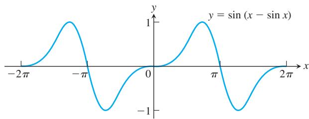
Analyzing Graphs
Each of the figures in Exercises 119 and 120 shows two graphs, the graph of a function
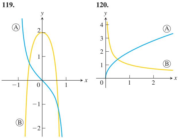
- Use the following information to graph the function
𝑦 = 𝑓 ( 𝑥 ) − 1 ≤ 𝑥 ≤ 6
i) The graph of
ii) The graph starts at the point
iii) The derivative of
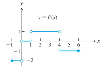
- Repeat Exercise 121, supposing that the graph starts at
( − 1 , 0 ) ( − 1 , 2 )
Logarithmic Differentiation
In Exercises 123–128, use logarithmic differentiation to find the derivative of y with respect to the appropriate variable.
-
𝑦 = 2 ( 𝑥 2 + 1 ) √ c o s 2 𝑥 -
𝑦 = 1 0 √ 3 𝑥 + 4 2 𝑥 − 4 -
𝑦 = ( ( 𝑡 + 1 ) ( 𝑡 − 1 ) ( 𝑡 − 2 ) ( 𝑡 + 3 ) ) 5 , 𝑡 > 2 -
𝑦 = 2 𝑢 2 𝑢 √ 𝑢 2 + 1 -
𝑦 = ( s i n 𝜃 ) √ 𝜃 -
𝑦 = ( l n 𝑥 ) 1 / ( l n 𝑥 )
Related Rates
- Right circular cylinder The total surface area S of a right circular cylinder is related to the base radius r and height h by the equation
𝑆 = 2 𝜋 𝑟 2 + 2 𝜋 𝑟 ℎ
a. How is
b. How is
c. How is
d. How is dr/dt related to dh/dt if S is constant?
- Right circular cone The lateral surface area
𝑆 𝑟 ℎ 𝑆 = 𝜋 𝑟 √ 𝑟 2 + ℎ 2
a. How is
b. How is
c. How is
-
Circle’s changing area The radius
𝑟 − 2 / 𝜋 m / s 𝑟 = 1 0 m -
Cube’s changing edges The volume of a cube is increasing at the rate of
1 2 0 0 c m 3 / m i n 2 0 c m -
Resistors connected in parallel If two resistors of
𝑅 1 𝑅 2
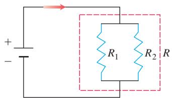
If
-
Impedance in a series circuit The impedance Z (ohms) in a series circuit is related to the resistance R (ohms) and reactance X (ohms) by the equation
𝑍 = √ 𝑅 2 + 𝑋 2 -
Speed of moving particle The coordinates of a particle moving in the metric xy-plane are differentiable functions of time t with dx/dt = 10 m/s and dy/dt = 5 m/s. How fast is the particle moving away from the origin as it passes through the point
( 3 , − 4 ) -
Motion of a particle A particle moves along the curve
𝑦 = 𝑥 3 / 2 𝑑 𝑥 / 𝑑 𝑡 𝑥 = 3 -
Draining a tank Water drains from the conical tank shown in the accompanying figure at the rate of
0 . 2 𝑚 3 / 𝑚 𝑖 𝑛
a. What is the relation between the variables h and r in the figure?
b. How fast is the water level dropping when h = 2 m?
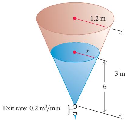
- Rotating spool As television cable is pulled from a large spool to be strung from the telephone poles along a street, it unwinds from the spool in layers of constant radius (see accompanying figure). If the truck pulling the cable moves at a steady 2 m/s (a touch over 7 km/h), use the equation
𝑠 = 𝑟 𝜃
- Moving searchlight beam The figure shows a boat 1 km offshore, sweeping the shore with a searchlight. The light turns at a constant rate,
𝑑 𝜃 / 𝑑 𝑡 = − 0 . 6
a. How fast is the light moving along the shore when it reaches point A?
b. How many revolutions per minute is 0.6 rad/s?
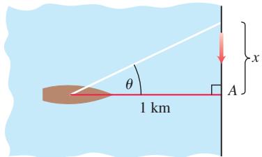
- Points moving on coordinate axes Points A and B move along the x- and y-axes, respectively, in such a way that the distance r (meters) along the perpendicular from the origin to the line AB remains constant. How fast is OA changing, and is it increasing or decreasing, when OB = 2r and B is moving toward O at the rate of 0.3r m/s?
Linearization
- Find the linearizations of
a.
Graph the curves and linearizations together.
- We can obtain a useful linear approximation of the function
𝑓 ( 𝑥 ) = 1 / ( 1 + t a n 𝑥 ) 𝑥 = 0
to get
Show that this result is the standard linear approximation of
-
Find the linearization of
𝑓 ( 𝑥 ) = √ 1 + 𝑥 + s i n 𝑥 − 0 . 5 -
Find the linearization of
𝑓 ( 𝑥 ) = 2 / ( 1 − 𝑥 ) + √ 1 + 𝑥 − 3 . 1
Differential Estimates of Change
- Surface area of a cone Write a formula that estimates the change that occurs in the lateral surface area of a right circular cone when the height changes from
ℎ 0 ℎ 0 + 𝑑 ℎ
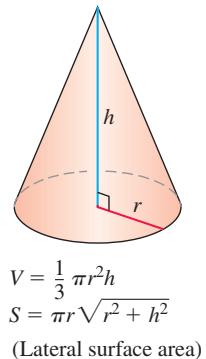
146. Controlling error
a. How accurately should you measure the edge of a cube to be reasonably sure of calculating the cube’s surface area with an error of no more than
b. Suppose that the edge is measured with the accuracy required in part (a). About how accurately can the cube’s volume be calculated from the edge measurement? To find out, estimate the percentage error in the volume calculation that might result from using the edge measurement.
- Compounding error The circumference of the equator of a sphere is measured as 10 cm with a possible error of 0.4 cm. This measurement is used to calculate the radius. The radius is then used to calculate the surface area and volume of the sphere. Estimate the percentage errors in the calculated values of
a. the radius. b. the surface area. c. the volume.
- Finding height To find the height of a lamppost (see accompanying figure), you stand a 1.8 m pole 10 m from the lamp and measure the length a of its shadow, finding it to be 4.5 m, give or take a centimeter. Calculate the height of the lamppost using the value a = 4.5, and estimate the possible error in the result.
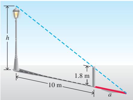
CHAPTER 3 Additional and Advanced Exercises
- An equation like
s i n 2 𝜃 + c o s 2 𝜃 = 1 𝜃 s i n 𝜃 = 0 . 5 𝜃 𝜃 𝜃
Differentiate the following to show that the resulting equations hold for all
a.
b.
-
If the identity
s i n ( 𝑥 + 𝑎 ) = s i n 𝑥 c o s 𝑎 + c o s 𝑥 s i n 𝑎 𝑥 2 − 2 𝑥 − 8 = 0 -
a. Find values for the constants
𝑎 , 𝑏 𝑐
satisfy the conditions
b. Find values for b and c that will make
satisfy the conditions
c. For the determined values of
4. Solutions to differential equations
a. Show that
b. How would you modify the functions in part (a) to satisfy the equation
Generalize this result.
-
An osculating circle Find the values of h, k, and a that make the circle
( 𝑥 − ℎ ) 2 + ( 𝑦 − 𝑘 ) 2 = 𝑎 2 𝑦 = 𝑥 2 + 1 𝑑 2 𝑦 / 𝑑 𝑥 2 -
Marginal revenue A bus will hold 60 people. The number x of people per trip who use the bus is related to the fare charged (p dollars) by the law
𝑝 = [ 3 − ( 𝑥 / 4 0 ) ] 2 𝑟 ( 𝑥 )
7. Industrial production
a. Economists often use the expression “rate of growth” in relative rather than absolute terms. For example, let
Let
b. Suppose that the labor force in part (a) is decreasing at the rate of 2% per year while the production per person is increasing at the rate of 3% per year. Is the total production increasing, or is it decreasing, and at what rate?
- Designing a gondola The designer of a 10 m-diameter spherical hot air balloon wants to suspend the gondola 2.5 m below the bottom of the balloon with cables tangent to the surface of the balloon, as shown. Two of the cables are shown running from the top edges of the gondola to their points of tangency,
( − 4 , − 3 ) ( 4 , − 3 )
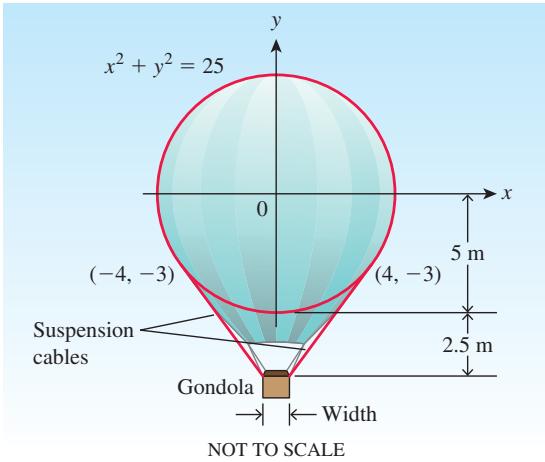
-
Pisa by parachute On August 5, 1988, Mike McCarthy of London jumped from the top of the Tower of Pisa. He then opened his parachute in what he said was a world record low-level parachute jump of 54.6 m. Make a rough sketch to show the shape of the graph of his speed during the jump. (Data from: Boston Globe, Aug. 6, 1988.)
-
Motion of a particle The position at time
𝑡 ≥ 0
a. What is the particle’s starting position
b. What are the points farthest to the left and right of the origin reached by the particle?
c. Find the particle’s velocity and acceleration at the points in part (b).
d. When does the particle first reach the origin? What are its velocity, speed, and acceleration then?
- Shooting a paper clip On Earth, you can easily shoot a paper clip 19.6 m straight up into the air with a rubber band. In t seconds after firing, the paper clip is
𝑠 = 1 9 . 6 𝑡 − 4 . 9 𝑡 2
a. How long does it take the paper clip to reach its maximum height? With what velocity does it leave your hand?
b. On the moon, the same acceleration will send the paper clip to a height of
-
Velocities of two particles At time t seconds, the positions of two particles on a coordinate line are
𝑠 1 = 3 𝑡 3 − 1 2 𝑡 2 + 1 8 𝑡 + 5 𝑠 2 = − 𝑡 3 + 9 𝑡 2 − 1 2 𝑡 -
Velocity of a particle A particle of constant mass m moves along the x-axis. Its velocity v and position x satisfy the equation
where
In Exercises 14 and 15, use implicit differentiation to find
14.
-
𝑦 𝑒 𝑥 = 𝑥 𝑦 + 1 -
Average and instantaneous velocity
a. Show that if the position x of a moving point is given by a quadratic function of
b. What is the geometric significance of the result in part (a)?
- Find all values of the constants m and b for which the function
is
a. continuous at
b. differentiable at
- Does the function
have a derivative at x = 0? Explain.
- a. For what values of
𝑎 𝑏
be differentiable for all values of x?
b. Discuss the geometry of the resulting graph of
- a. For what values of
𝑎 𝑏
be differentiable for all values of
b. Discuss the geometry of the resulting graph of g.
-
Odd differentiable functions Is there anything special about the derivative of an odd differentiable function of
𝑥 -
Even differentiable functions Is there anything special about the derivative of an even differentiable function of
𝑥 -
Suppose that the functions
𝑓 𝑔 𝑥 0 𝑓 𝑥 0 𝑓 ( 𝑥 0 ) = 0 𝑔 𝑥 0 𝑓 𝑔 𝑥 0 | 𝑥 | 𝑥 = 0 𝑥 | 𝑥 | 𝑥 = 0 -
(Continuation of Exercise 23.) Use the result of Exercise 23 to show that the following functions are differentiable at x = 0.
a.
b.
c.
d.
- Is the derivative of
continuous at x = 0? How about the derivative of
- Let
𝑓 ( 𝑥 ) = { 𝑥 2 , 𝑥 i s r a t i o n a l 0 , 𝑥 i s i r r a t i o n a l .
Show that
- Point B moves from point A to point C at 2 cm/s in the accompanying diagram. At what rate is
𝜃
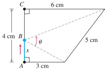
- Suppose that a function
𝑓 𝑥 𝑦
ii)
Show that the derivative
- The generalized product rule Use mathematical induction to prove that if
𝑦 = 𝑢 1 𝑢 2 ⋯ 𝑢 𝑛
- Leibniz’s rule for higher-order derivatives of products Leibniz’s rule for higher-order derivatives of products of differentiable functions says that
The equations in parts (a) and (b) are special cases of the equation in part (c). Derive the equation in part (c) by mathematical induction, using
- The period of a clock pendulum The period T of a clock pendulum (time for one full swing and back) is given by the formula
𝑇 2 = 4 𝜋 2 𝐿 / 𝑔 𝑔 = 9 . 8 𝑚 / 𝑠 2
a. the length of a clock pendulum whose period is T = 1 s.
b. the change dT in T if the pendulum in part (a) is lengthened 0.01 m.
c. the amount the clock gains or loses in a day as a result of the period’s changing by the amount
- The melting ice cube Assume that an ice cube retains its cubical shape as it melts. If we call its edge length s, its volume is
𝑉 = 𝑠 3 6 𝑠 2
The minus sign indicates that the volume is decreasing. We assume that the proportionality factor k is constant. (It probably depends on many things, such as the relative humidity of the surrounding air, the air temperature, and the incidence or absence of sunlight, to name only a few.) Assume a particular set of conditions in which the cube lost 1/4 of its volume during the first hour, and assume that the volume is
CHAPTER 3 Technology Application Projects
Mathematica/Maple Projects
Projects can be found at www.pearsonglobaleditions.com or within MyLab Math.
You will visualize the secant line between successive points on a curve and observe what happens as the distance between them becomes small. The function, sample points, and secant lines are plotted on a single graph, while a second graph compares the slopes of the secant lines with the derivative function.
- Derivatives, Slopes, Tangent Lines, and Making Movies Parts I–III. You will visualize the derivative at a point, the linearization of a function, and the derivative of a function. You will learn how to plot the function and selected tangent lines on the same graph. Part IV (Plotting Many Tangent Lines)
Part V (Making Movies). Parts IV and V of the module can be used to animate tangent lines as one moves along the graph of a function.
-
Convergence of Secant Slopes to the Derivative Function You will visualize right-hand and left-hand derivatives.
-
Motion Along a Straight Line: Position
→ →