Chapter 16: First-Order Differential Equations

Chapter 17 is available online.

To access this chapter, visit the companion Website.

教材插图

OVERVIEW Many real-world problems, when formulated mathematically, lead to differential equations. We encountered a number of these equations in previous chapters when studying phenomena such as the motion of an object along a straight line, the decay of a radioactive material, the growth of a population, and the cooling of a heated object placed within a medium of lower temperature.

Section 4.8 introduced diferential equations of the form $𝑑 𝑦 / 𝑑 𝑥 = 𝑓 (𝑥)$ , where f is given and $𝑦$ is an unknown function of x. We learned that when f is continuous over some interval, the general solution $𝑦 (𝑥)$ is found directly by integration, $𝑦 = \int 𝑓 (𝑥)$ dx . In Section 7.2 we investigated diferential equations of the form $𝑑 𝑦 / 𝑑 𝑥 : = : 𝑓 (𝑥, 𝑦)$ , where $𝑓$ is a function of both the independent variable x and the dependent variable y. There we learned how to find the general solution for the special case when the diferential equation is separable. In this chapter we further extend our study to include other commonly occurring first-order diferential equations. These diferential equations involve only first derivatives of the unknown function y x( ), and they model phenomena varying from simple electrical circuits to the concentration of a chemical in a container. Diferential equations involving second derivatives are examined in Chapter 17.

16.1 Solutions, Slope Fields, and Euler’s Method

We begin this section by defining general differential equations involving first derivatives. We then look at slope fields, which give a geometric picture of the solutions to such equations. Many differential equations cannot be solved by obtaining an explicit formula for the solution. However, we can often find numerical approximations to solutions. We present one such method here, called Euler’s method, which is the basis for many other numerical methods as well.

General First-Order Differential Equations and Solutions

A first-order differential equation is an equation

𝑑 𝑦 𝑑 𝑥 = 𝑓 (𝑥, 𝑦) (1)

in which $𝑓 (𝑥, 𝑦)$ is a function of two variables defined on a region in the xy-plane. The equation is of first order because it involves only the first derivative $𝑑 𝑦 / 𝑑 𝑥$ and not higher-order derivatives. In a typical situation y represents an unknown function of $𝑥,$ and $𝑓 (𝑥, 𝑦)$ is a known function. Some examples of first-order differential equations are $𝑦' = 𝑥 + 𝑦, 𝑦' = 𝑦 / 𝑥$ , and $𝑦' = 3 𝑥 𝑦$ . In all cases we should think of y as an unknown function of x whose derivative is given by $𝑓 (𝑥, 𝑦)$ . The equations

𝑦' = 𝑓 (𝑥, 𝑦) a n d 𝑑 𝑑 𝑥 𝑦 = 𝑓 (𝑥, 𝑦)

are equivalent to Equation (1), and all three forms will be used interchangeably in the text.

A solution of Equation (1) is a differentiable function $𝑦 = 𝑦 (𝑥)$ defined on an interval I of x-values (possibly an infinite interval) such that

𝑑 𝑑 𝑥 𝑦 (𝑥) = 𝑓 (𝑥, 𝑦 (𝑥))

on that interval. That is, when y x( ) and its derivative $𝑦' (𝑥)$ are substituted into Equation (1), the resulting equation is true for all x over the interval I.

EXAMPLE 1 Show that every member of the family of functions

𝑦 = 𝐶 𝑥 + 2

is a solution of the first-order differential equation

𝑑 𝑦 𝑑 𝑥 = 1 𝑥 (2 - 𝑦)

on the interval $(0, \infty)$ , where C is any constant.

Solution Differentiating $𝑦 = 𝐶 / 𝑥 + 2$ gives

𝑑 𝑦 𝑑 𝑥 = 𝐶 𝑑 𝑑 𝑥 (1 𝑥) + 0 = - 𝐶 𝑥 2 .

We need to show that the differential equation is satisfied when we substitute into it the expressions $(𝐶 / 𝑥) + 2$ for y, and $- 𝐶 / 𝑥 2$ for $𝑑 𝑦 / 𝑑 𝑥$ . That is, we need to verify that for all $𝑥 \in (0, \infty)$

- 𝐶 𝑥 2 = 1 𝑥 [2 - (𝐶 𝑥 + 2)] .

This last equation follows immediately by expanding the expression on the right-hand side:

1 𝑥 [2 - (𝐶 𝑥 + 2)] = 1 𝑥 (- 𝐶 𝑥) = - 𝐶 𝑥 2 .

Therefore, for every value of C, the function $𝑦 = 𝐶 / 𝑥 + 2$ is a solution of the differential equation. ■

The differential equation in Example 1 has a whole family of solutions, one for each value of C. A natural question to consider is whether this family contains all the solutions to the differential equation, or whether there are others that can somehow arise. The general solution to a first-order differential equation is the name given to an expression that contains all possible solutions. The general solution always contains an arbitrary constant, but a solution may contain an arbitrary constant without being the general solution. Establishing when a solution is the general solution is left to a more extensive development of the theory of differential equations.

As with antiderivatives, we often need a particular rather than the general solution to a first-order differential equation $𝑦' = 𝑓 (𝑥, 𝑦)$ . A common way to pick out one of the collection of possible solutions is to specify the value of y at a point $𝑥 = 𝑥 0 .$ The particular solution satisfying the initial condition $𝑦 (𝑥 0) = 𝑦 0$ is the solution $𝑦 = 𝑦 (𝑥)$ whose value is $𝑦 0$ when $𝑥 = 𝑥 0 .$ Thus the graph of the particular solution passes through the point $(𝑥 0, 𝑦 0)$ in the xy-plane. A first-order initial value problem is a differential equation $𝑦' = 𝑓 (𝑥, 𝑦)$ whose solution must satisfy an initial condition $𝑦 (𝑥 0) = 𝑦 0$

EXAMPLE 2 Show that the function

𝑦 = (𝑥 + 1) - 13 𝑒 𝑥

is a solution to the first-order initial value problem

𝑑 𝑦 𝑑 𝑥 = 𝑦 - 𝑥, 𝑦 (0) = 23 .

Solution The equation

𝑑 𝑦 𝑑 𝑥 = 𝑦 - 𝑥

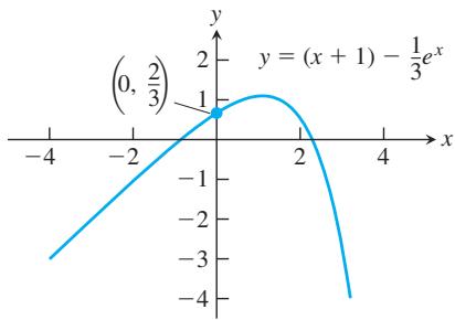
FIGURE 16.1 Graph of the solution to the initial value problem in Example 2.

教材插图

is a first-order differential equation with $𝑓 (𝑥, 𝑦) = 𝑦 - 𝑥 .$

On the left side of the equation:

𝑑 𝑦 𝑑 𝑥 = 𝑑 𝑑 𝑥 (𝑥 + 1 - 13 𝑒 𝑥) = 1 - 13 𝑒 𝑥 .

On the right side of the equation:

𝑦 - 𝑥 = (𝑥 + 1) - 13 𝑒 𝑥 - 𝑥 = 1 - 13 𝑒 𝑥 .

The function satisfies the initial condition because

𝑦 (0) = [(𝑥 + 1) - 13 𝑒 𝑥] 𝑥 = 0 = 1 - 13 = 23 .

The graph of the function is shown in Figure 16.1.

Slope Fields: Viewing Solution Curves

Each time we specify an initial condition $𝑦 (𝑥 0) = 𝑦 0$ for the solution of a differential equation $𝑦' = 𝑓 (𝑥, 𝑦)$ , the solution curve (graph of the solution) is required to pass through the point $(𝑥 0, 𝑦 0)$ and to have slope $𝑓 (𝑥 0, 𝑦 0)$ there. We can picture these slopes graphically by drawing short line segments of slope $𝑓 (𝑥, 𝑦)$ at selected points $(𝑥, 𝑦)$ in the region of the xy-plane that constitutes the domain of f. Each segment has the same slope as the solution curve through $(𝑥, 𝑦)$ and so is tangent to the curve there. The resulting picture is called a slope field (or direction field) and gives a visualization of the general shape of the solution curves. Figure 16.2a shows a slope field, with a particular solution sketched into it in Figure 16.2b. We see how these line segments indicate the direction the solution curve takes at each point it passes through.

教材插图

(a)

教材插图

(b)

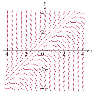
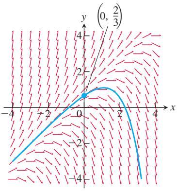
FIGURE 16.2 (a) Slope field for $𝑑 𝑦 𝑑 𝑥 = 𝑦 - 𝑥 .$ (b) The particular solution curve through the point $(0, 23) (E x a m p l e 2)$

(a)

教材插图

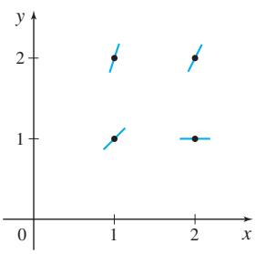
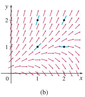
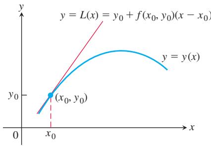
FIGURE 16.3 (a) The slope field for $𝑦' = 2 𝑦 - 𝑥$ is shown at four points. (b) The slope field at several hundred additional points in the plane.

教材插图

FIGURE 16.5 The linearization L x( ) of $𝑦 = 𝑦 (𝑥) a t 𝑥 = 𝑥 0$

EXAMPLE 3 For the differential equation

𝑦' = 2 𝑦 - 𝑥,

draw line segments representing the slope field at the points (1, 2 , ) (1, 1 , ) (2, 2 , and ) (2, 1 .)

Solution $A t (1, 2)$ the slope is $2 (2) - (1) = 3$ . Similarly, the slope at ( 2, 2 is 2, at ) ( 2, 1) is 0, and at (1, 1 is 1. We indicate this on the graph by drawing short line segments of the) given slope through each point, as in Figure 16.3. ■

Figure 16.4 shows three slope fields, and we see how the solution curves behave by following the tangent line segments in these fields. Slope fields are useful because they display the overall behavior of the family of solution curves for a given differential equation. For instance, the slope field in Figure 16.4b reveals that every solution y x( ) to the differential equation specified in the figure satisfies $l i m 𝑥 \to \pm \infty 𝑦 (𝑥) = 0$ . We will see that knowing the overall behavior of the solution curves is often critical to understanding and predicting outcomes in a real-world system modeled by a differential equation.

Constructing a slope field with pencil and paper can be quite tedious. Our examples were generated by computer software.

教材插图

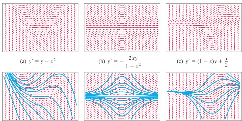
FIGURE 16.4 Slope fields (top row) and selected solution curves (bottom row). In computer renditions, slope segments are sometimes portrayed with arrows, as they are here, but they should be considered as just tangent line segments.

Euler’s Method

If we do not require or cannot find an exact solution that gives an explicit formula for an initial value problem $𝑦' = 𝑓 (𝑥, 𝑦), 𝑦 (𝑥 0) = 𝑦 0$ , we can often use a computer to generate a table of approximate numerical values of y for values of x in an appropriate interval. Such a table is called a numerical solution of the problem, and the process by which we generate the table is called a numerical method.

Given a differential equation $𝑑 𝑦 / 𝑑 𝑥 = 𝑓 (𝑥, 𝑦)$ and an initial condition $𝑦 (𝑥 0) = 𝑦 0$ we can approximate the solution $𝑦 = 𝑦 (𝑥)$ by its linearization

𝐿 (𝑥) = 𝑦 (𝑥 0) + 𝑦' (𝑥 0) (𝑥 - 𝑥 0) o r 𝐿 (𝑥) = 𝑦 0 + 𝑓 (𝑥 0, 𝑦 0) (𝑥 - 𝑥 0) .

The function L x( ) gives a good approximation to the solution $𝑦 (𝑥)$ in a short interval about $𝑥 0 (F i g u r e 16.5)$ . The basis of Euler’s method is to patch together a string of linearizations to approximate the curve over a longer stretch. Here is how the method works.

We know the point $(𝑥 0, 𝑦 0)$ lies on the solution curve. Suppose that we specify a new value for the independent variable to be $𝑥 1 = 𝑥 0 + 𝑑 𝑥 .$ . (Recall that $𝑑 𝑥 = Δ 𝑥$ in the definition of differentials.) If the increment dx is small, then

𝑦 1 = 𝐿 (𝑥 1) = 𝑦 0 + 𝑓 (𝑥 0, 𝑦 0) 𝑑 𝑥

教材插图

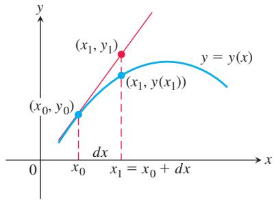
FIGURE 16.6 The first Euler step approximates $𝑦 (𝑥 1)$ with $𝑦 1 = 𝐿 (𝑥 1)$

教材插图

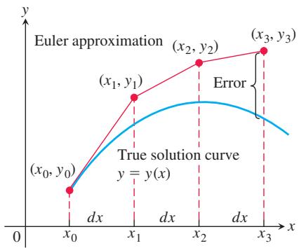
FIGURE 16.7 Three steps in the Euler approximation to the solution of the initial value problem $𝑦' = 𝑓 (𝑥, 𝑦), 𝑦 (𝑥 0) = 𝑦 0 .$ As we take more steps, the errors involved usually accumulate, but not in the exaggerated way shown here.

is a good approximation to the exact solution value $𝑦 = 𝑦 (𝑥 1)$ . So from the point $(𝑥 0, 𝑦 0)$ which lies exactly on the solution curve, we have obtained the point $(𝑥 1, 𝑦 1)$ , which lies very close to the point $(𝑥 1, 𝑦 (𝑥 1))$ on the solution curve (Figure 16.6).

Using the point $(𝑥 1, 𝑦 1)$ and the slope $𝑓 (𝑥 1, 𝑦 1)$ of the solution curve through $(𝑥 1, 𝑦 1)$ we take a second step. Setting $𝑥 2 = 𝑥 1 + 𝑑 𝑥$ , we use the linearization of the solution curve through $(𝑥 1, 𝑦 1)$ to calculate

𝑦 2 = 𝑦 1 + 𝑓 (𝑥 1, 𝑦 1) 𝑑 𝑥 .

This gives the next approximation $(𝑥 2, 𝑦 2)$ to values along the solution curve $𝑦 = 𝑦 (𝑥)$ (Figure 16.7). Continuing in this fashion, we take a third step from the point $(𝑥 2, 𝑦 2)$ with slope $𝑓 (𝑥 2, 𝑦 2)$ to obtain the third approximation

𝑦 3 = 𝑦 2 + 𝑓 (𝑥 2, 𝑦 2) 𝑑 𝑥,

and so on. We are building an approximation to a solution by following the direction of the slope field of the differential equation.

The steps in Figure 16.7 are drawn large to illustrate the construction process, so the approximation looks crude. In practice, dx would be chosen small enough to make the red curve hug the blue one and give a better approximation.

EXAMPLE 4 Find the first three approximations $𝑦 1, 𝑦 2, 𝑦 3$ using Euler’s method for the initial value problem

𝑦' = 1 + 𝑦, 𝑦 (0) = 1,

starting at $𝑥 0 = 0 w i t h 𝑑 𝑥 = 0.1$

Solution We already have the starting values $𝑥 0 = 0$ and $𝑦 0 = 1$ . Next we determine the values of x at which the Euler approximations will take place: $𝑥 1 = 𝑥 0 + 𝑑 𝑥 = 0.1$ $𝑥 2 = 𝑥 0 + 2 𝑑 𝑥 = 0.2 /$ and $𝑥 3 = 𝑥 0 + 3 𝑑 𝑥 = 0.3$ . Then we find

F i r s t : 𝑦 1 = 𝑦 0 + 𝑓 (𝑥 0, 𝑦 0) 𝑑 𝑥 = 𝑦 0 + (1 + 𝑦 0) 𝑑 𝑥 𝑓 (𝑥, 𝑦) = 1 + 𝑦 = 1 + (1 + 1) (0 . 1) = 1 . 2 𝑦 0 = 1, 𝑑 𝑥 = 0 . 1

Second:

𝑦 2 = 𝑦 1 + 𝑓 (𝑥 1, 𝑦 1) 𝑑 𝑥 = 𝑦 1 + (1 + 𝑦 1) 𝑑 𝑥 = 1 . 2 + (1 + 1 . 2) (0 . 1) = 1 . 42 𝑦 1 = 1 . 2, 𝑑 𝑥 = 0 . 1

T h i r d : 𝑦 3 = 𝑦 2 + 𝑓 (𝑥 2, 𝑦 2) 𝑑 𝑥 = 𝑦 2 + (1 + 𝑦 2) 𝑑 𝑥 = 1 . 42 + (1 + 1 . 42) (0 . 1) = 1 . 662 𝑦 2 = 1 . 42, 𝑑 𝑥 = 0 . 1

The step-by-step process used in Example 4 can be continued with more points. Using equally spaced values for the independent variable in the table for the numerical solution, and generating n of them, set

𝑥 1 = 𝑥 0 + 𝑑 𝑥 𝑥 2 = 𝑥 1 + 𝑑 𝑥 ⋮ 𝑥 𝑛 = 𝑥 𝑛 - 1 + 𝑑 𝑥 .

Then calculate the approximations to the solution,

𝑦 1 = 𝑦 0 + 𝑓 (𝑥 0, 𝑦 0) 𝑑 𝑥 𝑦 2 = 𝑦 1 + 𝑓 (𝑥 1, 𝑦 1) 𝑑 𝑥 ⋮ 𝑦 𝑛 = 𝑦 𝑛 - 1 + 𝑓 (𝑥 𝑛 - 1, 𝑦 𝑛 - 1) 𝑑 𝑥 .

HISTORICAL BIOGRAPHY

Leonhard Euler

(1707–1783)

Born in Basel, Switzerland, Leonhard Euler was the dominant mathematical figure of his century and the most prolific mathematician who ever lived. He was also an astronomer, physicist, engineer, and chemist. He was the first scientist to give the function concept prominence in his work, thereby setting a strong foundation for the development of calculus and other areas of mathematics.

To know more, visit the companion Website.

教材插图

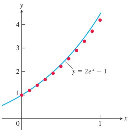
FIGURE 16.8 The graph of FIGURE 16.8 The graph of

$𝑦 = 2 𝑒 𝑥 - 1$ 1 superimposed on a scatterplot of the Euler approximations shown in Table 16.1 (Example 5).

The number of steps n can be as large as we like, but errors involving the representation of numbers in software can accumulate if n is too large.

Euler’s method is easy to implement on a computer or calculator. A typical software program takes as input $𝑥 0$ and $𝑦 0 .$ , the number of steps n, and the step size dx. It then calculates the approximate solution values $𝑦 1, 𝑦 2, . . ., 𝑦 𝑛$ in iterative fashion, as just described.

Solving the separable equation in Example 4, we find that the exact solution to the initial value problem is $𝑦 = 2 𝑒 𝑥 - 1$ . We use this information in Example 5.

EXAMPLE 5 Use Euler’s method to solve

𝑦' = 1 + 𝑦, 𝑦 (0) = 1,

on the interval $0 \leq 𝑥 \leq 1$ , starting at $𝑥 0 = 0$ and taking (a) $𝑑 𝑥 = 0.1$ and $(𝐛) 𝑑 𝑥 = 0.05$ Compare the approximations with the values of the exact solution $𝑦 = 2 𝑒 𝑥 - 1$

Solution

(a) We used a computer to generate the approximate values in Table 16.1. The “error” column is obtained by subtracting the unrounded Euler values from the unrounded values found using the exact solution. All entries are then rounded to four decimal places.

TABLE 16.1 Euler solution of $𝑦' = 1 + 𝑦, 𝑦 (0) = 1,$ step size dx = 0.1

x	y (Euler)	y (exact)	Error
0	1	1	0
0.1	1.2	1.2103	0.0103
0.2	1.42	1.4428	0.0228
0.3	1.662	1.6997	0.0377
0.4	1.9282	1.9836	0.0554
0.5	2.2210	2.2974	0.0764
0.6	2.5431	2.6442	0.1011
0.7	2.8974	3.0275	0.1301
0.8	3.2872	3.4511	0.1639
0.9	3.7159	3.9192	0.2033
1.0	4.1875	4.4366	0.2491

By the time we reach x = 1 (after 10 steps), the error is about 5.6% of the exact solution. A plot of the exact solution curve with the scatterplot of Euler solution points from Table 16.1 is shown in Figure 16.8.

(b) One way to try to reduce the error is to decrease the step size. Table 16.2 shows the results and their comparisons with the exact solutions when we decrease the step size to 0.05, doubling the number of steps to 20. As in Table 16.1, all computations are performed before rounding. This time when we reach x = 1, the relative error is only about 2.9%. 1

It might be tempting to reduce the step size even further in Example 5 to obtain greater accuracy. Each additional calculation, however, not only requires additional computer time but, more importantly, adds to the buildup of round-off errors due to the approximate representations of numbers inside the computer.

y x y ′ = +

The analysis of error and the investigation of methods to reduce it when making numerical calculations are important. An area of mathematics called numerical analysis studies advanced numerical methods that are more accurate than Euler’s method.

TABLE 16.2 Euler solution of $\boldsymbol𝐲′=𝟏+\boldsymbol𝑦,\boldsymbol𝐲(𝟎)=𝟏,$ step size dx = 0.05

x	y (Euler)	y (exact)	Error
0	1	1	0
0.05	1.1	1.1025	0.0025
0.10	1.205	1.2103	0.0053
0.15	1.3153	1.3237	0.0084
0.20	1.4310	1.4428	0.0118
0.25	1.5526	1.5681	0.0155
0.30	1.6802	1.6997	0.0195
0.35	1.8142	1.8381	0.0239
0.40	1.9549	1.9836	0.0287
0.45	2.1027	2.1366	0.0340
0.50	2.2578	2.2974	0.0397
0.55	2.4207	2.4665	0.0458
0.60	2.5917	2.6442	0.0525
0.65	2.7713	2.8311	0.0598
0.70	2.9599	3.0275	0.0676
0.75	3.1579	3.2340	0.0761
0.80	3.3657	3.4511	0.0853
0.85	3.5840	3.6793	0.0953
0.90	3.8132	3.9192	0.1060
0.95	4.0539	4.1714	0.1175
1.00	4.3066	4.4366	0.1300

EXERCISES 16.1

Slope Fields

In Exercises 1–4, match the differential equations with their slope fields, graphed here.

教材插图

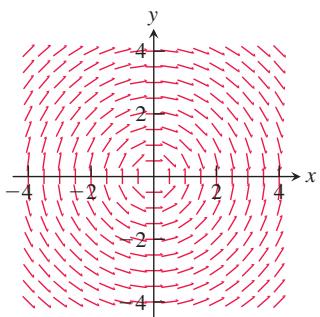
(a)

教材插图

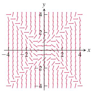
(b)

教材插图

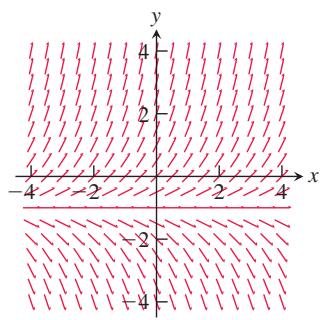
(c)

𝑦' = - 𝑥 𝑦

教材插图

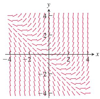
(d)

y y ′ = + 1
$𝑦' = 𝑦 2 - 𝑥 2$

In Exercises 5 and 6, copy the slope fields, and sketch in some of the solution curves.

𝑦' = (𝑦 + 2) (𝑦 - 2)

教材插图

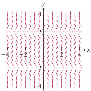
$𝑦' = 𝑦 (𝑦 + 1) (𝑦 - 1)$

教材插图

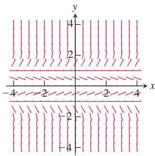
Integral Equations

In Exercises 7–12, write an equivalent first-order differential equation and initial condition for y.

$𝑦 = - 1 + \int 𝑥 1 (𝑡 - 𝑦 (𝑡)) 𝑑 𝑡 8 . 𝑦 = \int 𝑥 1 1 𝑡 𝑑 𝑡$
$𝑦 = 2 - \int 𝑥 0 (1 + 𝑦 (𝑡)) 𝑑 𝑡$ t dtsin
$𝑦 = 1 + \int 𝑥 0 𝑦 (𝑡) 𝑑 𝑡$
$𝑦 = 𝑥 + 4 + \int 𝑥 - 2 𝑡 𝑒 𝑦 (𝑡) 𝑑 𝑡$
$𝑦 = l n 𝑥 + \int 𝑒 𝑥 \sqrt 𝑡 2 + (𝑦 (𝑡)) 2 𝑑 𝑡$

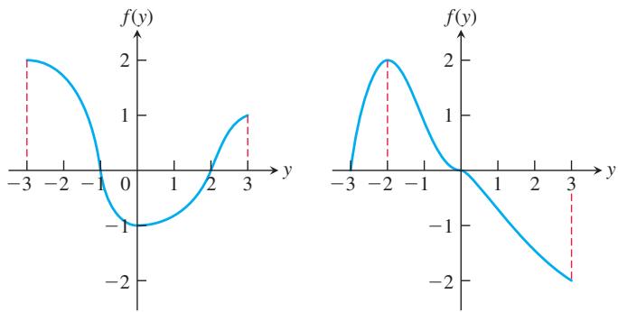
In Exercises 13 and 14, consider the differential equation $𝑦' = 𝑓 (𝑦)$ and the given graph of f. Make a rough sketch of a direction field for each differential equation.

教材插图

Using Euler’s Method

In Exercises 15–20, use Euler’s method to calculate the first three approximations to the given initial value problem for the specified increment size. Calculate the exact solution and investigate the accuracy of your approximations. Round your results to four decimal places.

$𝑦' = 2 𝑦 𝑥, 𝑦 (1) = - 1, 𝑑 𝑥 = 0.5$
$𝑦' = 𝑥 (1 - 𝑦), 𝑦 (1) = 0, 𝑑 𝑥 = 0.2$
$𝑦' = 2 𝑥 𝑦 + 2 𝑦, 𝑦 (0) = 3, 𝑑 𝑥 = 0.2$
y y x y dx 1 2 , ( 1) 1, 0.5 2 ′ = + − = = ( )

19.T $𝑦' = 2 𝑥 𝑒 𝑥 2, 𝑦 (0) = 2, 𝑑 𝑥 = 0.1$

20.T $𝑦' = 𝑦 𝑒 𝑥, 𝑦 (0) = 2, 𝑑 𝑥 = 0.5$

Use Euler’s method with dx = 0.2 to estimate y(1) if y y′ = and y(0) 1. = What is the exact value of y(1)?
Use Euler’s method with dx = 0.2 to estimate y(2) if $𝑦' = 𝑦 / 𝑥$ and y(1) 2.= What is the exact value of y(2)?
Use Euler’s method with dx = 0.5 to estimate y(5) if $𝑦' = 𝑦 2 / \sqrt 𝑥$ and y(1) 1.= − What is the exact value of y(5)?
Use Euler’s method with dx = 1 3 to estimate y(2) if y x y ′ = sin and y(0) 1.= What is the exact value of y(2)?
Show that the solution of the initial value problem

𝑦' = 𝑥 + 𝑦, 𝑦 (𝑥 0) = 𝑦 0

𝑦 = - 1 - 𝑥 + (1 + 𝑥 0 + 𝑦 0) 𝑒 𝑥 - 𝑥 0 .

What integral equation is equivalent to the initial value problem $𝑦' = 𝑓 (𝑥), 𝑦 (𝑥 0) = 𝑦 0 ?$

COMPUTER EXPLORATIONS

In Exercises 27–32, obtain a slope field and add to it graphs of the solution curves passing through the given points.

y y ′ = with a. (0, 1) b. ( 0, 2) c. ( 0, 1 − )
$𝑦' = 2 (𝑦 - 4)$ with a. (0, 1) b. (0, 4) c. (0, 5)
$𝑦' = 𝑦 (𝑥 + 𝑦)$ with a. (0, 1) b. (0, 2 − ) c. (0, 1 4) d. (− −1, 1)
y y 2 ′ = with a. (0, 1) b. ( 0, 2) c. ( 0, 1 − ) d. (0, 0)
$𝑦' = (𝑦 - 1) (𝑥 + 2) w i t h 𝐚 . (0, - 1) 𝐛 . (0, 1)$ c. (0, 3) d. (1, 1 − )
$𝑦' = 𝑥 𝑦 𝑥 2 + 4$ with a. (0, 2) b. ( 0, 6 − ) c. $(- 2 \sqrt 3, - 4)$

In Exercises 33 and 34, obtain a slope field, and graph the particular solution over the specified interval. Use your CAS DE solver to find the general solution of the differential equation.

A logistic equation $𝑦' = 𝑦 (2 - 𝑦), 𝑦 (0) = 1 / 2; 0 \leq 𝑥 \leq 4,$ $0 \leq 𝑦 \leq 3$
$𝑦' = (s i n 𝑥) (s i n 𝑦), 𝑦 (0) = 2; - 6 \leq 𝑥 \leq 6, - 6 \leq 𝑦 \leq 6$

Exercises 35 and 36 have no explicit solution in terms of elementary functions. Use a CAS to explore graphically each of the differential equations.

𝑦' = c o s (2 𝑥 - 𝑦), 𝑦 (0) = 2; 0 \leq 𝑥 \leq 5, 0 \leq 𝑦 \leq 5

A Gompertz equation $𝑦' = 𝑦 (1 / 2 - l n 𝑦), 𝑦 (0) = 1 / 3;$ $0 \leq 𝑥 \leq 4, 0 \leq 𝑦 \leq 3$
Use a CAS to find the solutions of $𝑦' + 𝑦 = 𝑓 (𝑥)$ , subject to the initial condition $𝑦 (0) = 0, i f 𝑓 (𝑥)$ is

a. 2x b. sin 2x c. 3e ^x ² d. 2 cos 2 .e x^−x ²

Graph all four solutions over the interval $- 2 \leq 𝑥 \leq 6$ to compare the results.

a. Use a CAS to plot the slope field of the differential equation

𝑦' = 3 𝑥 2 + 4 𝑥 + 2 2 (𝑦 - 1)

over the region $- 3 \leq 𝑥 \leq 3 a n d - 3 \leq 𝑦 \leq 3 .$

b. Separate the variables and use a CAS integrator to find the general solution in implicit form.

c. Using a CAS implicit function grapher, plot solution curves for the arbitrary constant values $𝐶 = - 6, - 4, - 2, 0, 2, 4, 6 .$

d. Find and graph the solution that satisfies the initial condition y(0) 1. = −

In Exercises 39–42, use Euler’s method with the specified step size to estimate the value of the solution at the given point $𝑥 *$ . Find the value of the exact solution at $𝑥 *$

$𝑦' = 2 𝑥 𝑒 𝑥 2, 𝑦 (0) = 2, 𝑑 𝑥 = 0 . 1, 𝑥 * = 1$
$𝑦' = 2 𝑦 2 (𝑥 - 1), 𝑦 (2) = - 1 / 2, 𝑑 𝑥 = 0 . 1, 𝑥 * = 3$
$𝑦' = \sqrt 𝑥 / 𝑦, 𝑦 > 0, 𝑦 (0) = 1, 𝑑 𝑥 = 0.1, 𝑥 * = 1$
$𝑦' = 1 + 𝑦 2, 𝑦 (0) = 0, 𝑑 𝑥 = 0.1, 𝑥 * = 1$

Use a CAS to explore graphically each of the differential equations in Exercises 43–46. Perform the following steps to help with your explorations.

a. Plot a slope field for the differential equation in the given xy-window.

b. Find the general solution of the differential equation using your CAS DE solver.

c. Graph the solutions for the values of the arbitrary constant $𝐶 - = - 2, - 1, 0, 1, 2$ superimposed on your slope field plot.

d. Find and graph the solution that satisfies the specified initial condition over the interval [ ] 0, . b

e. Find the Euler numerical approximation to the solution of the initial value problem with 4 subintervals of the x-interval, and plot the Euler approximation superimposed on the graph produced in part (d).

f. Repeat part (e) for 8, 16, and 32 subintervals. Plot these three Euler approximations superimposed on the graph from part (e).

g. Find the error ( y y( ) exact Euler− ( )) at the specified point x = b for each of your four Euler approximations. Discuss the improvement in the percentage error.

43 . 𝑦' = 𝑥 + 𝑦, 𝑦 (0) = - 7 / 10; - 4 \leq 𝑥 \leq 4, - 4 \leq 𝑦 \leq 4; 𝑏 = 1 44 . $ $ 𝑦' = - 𝑥 / 𝑦, 𝑦 (0) = 2; - 3 \leq 𝑥 \leq 3, - 3 \leq 𝑦 \leq 3; 𝑏 = 2 $ $ 45 . 𝑦' = 𝑦 (2 - 𝑦), 𝑦 (0) = 1 / 2; 0 \leq 𝑥 \leq 4, 0 \leq 𝑦 \leq 3; 𝑏 = 3

46 . 𝑦' = (s i n 𝑥) (s i n 𝑦), 𝑦 (0) = 2; - 6 \leq 𝑥 \leq 6, - 6 \leq 𝑦 \leq 6; 𝑏 = 3 𝜋 / 2

16.2 First-Order Linear Equations

A first-order linear differential equation is one that can be written in the form

𝑑 𝑦 𝑑 𝑥 + 𝑃 (𝑥) 𝑦 = 𝑄 (𝑥), (1)

where P and Q are continuous functions of x. Equation (1) is the linear equation’s standard form. Since the exponential growth decay equation $𝑑 𝑦 / 𝑑 𝑥 : = : 𝑘 𝑦$ (Section 7.2) can be put in the standard form

𝑑 𝑦 𝑑 𝑥 - 𝑘 𝑦 = 0,

we see it is a linear equation with $𝑃 (𝑥) = - 𝑘 a n d 𝑄 (𝑥) = 0 .$ . Equation (1) is linear (in y) because y and its derivative dy dx occur only to the first power, they are not multiplied together, nor do they appear as the argument of a function (such as sin $𝑦, 𝑒 𝑦, o r \sqrt 𝑑 𝑦 / 𝑑 𝑥)$

EXAMPLE 1 Put the following equation in standard form:

𝑥 𝑑 𝑦 𝑑 𝑥 = 𝑥 2 + 3 𝑦, 𝑥 > 0 .

Solution

𝑥 𝑑 𝑦 𝑑 𝑥 = 𝑥 2 + 3 𝑦 𝑑 𝑦 𝑑 𝑥 = 𝑥 + 3 𝑥 𝑦 D i v i d e b y 𝑥 . 𝑑 𝑦 𝑑 𝑥 - 3 𝑥 𝑦 = 𝑥 S t a n d a r d f o r m w i t h 𝑃 (𝑥) = - 3 / 𝑥 a n d 𝑄 (𝑥) = 𝑥

Notice that $𝑃 (𝑥)$ is $- 3 / 𝑥$ , not $+ 3 / 𝑥$ . The standard form is $𝑦' + 𝑃 (𝑥) 𝑦 = 𝑄 (𝑥)$ , so the minus sign is part of the formula for $𝑃 (𝑥)$ ■

Solving Linear Equations

We solve the equation

𝑑 𝑦 𝑑 𝑥 + 𝑃 (𝑥) 𝑦 = 𝑄 (𝑥)

by multiplying both sides by a positive function $𝑣 (𝑥)$ that transforms the left-hand side into the derivative of the product $𝑣 (𝑥) \cdot 𝑦 .$ We will show how to find υ in a moment, but first we want to show how, once found, it provides the solution we seek.

Here is why multiplying by υ( ) x works:

𝑑 𝑦 𝑑 𝑥 + 𝑃 (𝑥) 𝑦 = 𝑄 (𝑥) O r i g i n a l e q u a t i o n i s i n s t a n d a r d f o r m . 𝑣 (𝑥) 𝑑 𝑦 𝑑 𝑥 + 𝑃 (𝑥) 𝑣 (𝑥) 𝑦 = 𝑣 (𝑥) 𝑄 (𝑥) M u l t i p l y b y p o s i t i v e 𝑣 (𝑥) . 𝑑 𝑑 𝑥 (𝑣 (𝑥) \cdot 𝑦) = 𝑣 (𝑥) 𝑄 (𝑥) 𝑣 (𝑥) i s c h o s e n t o m a k e 𝑣 𝑑 𝑦 𝑑 𝑥 + 𝑃 𝑣 𝑦 = 𝑑 𝑑 𝑥 (𝑣 \cdot 𝑦) . 𝑣 (𝑥) \cdot 𝑦 = \int 𝑣 (𝑥) 𝑄 (𝑥) 𝑑 𝑥 I n t e g r a t e w i t h r e s p e c t t o 𝑥 . 𝑦 = 1 𝑣 (𝑥) \int 𝑣 (𝑥) 𝑄 (𝑥) 𝑑 𝑥 D i v i d e b y 𝑣 (𝑥) . (2)

Equation (2) expresses the solution of Equation (1) in terms of the functions $𝑣 (𝑥)$ and $𝑄 (𝑥)$ . We call υ( )x an integrating factor for Equation (1) because its presence makes the equation integrable.

Why doesn’t the formula for $𝑃 (𝑥)$ appear in the solution as well? It does, but indirectly, in the construction of the positive function $𝑣 (𝑥)$ . We have

𝑑 𝑑 𝑥 (𝑣 𝑦) = 𝑣 𝑑 𝑦 𝑑 𝑥 + 𝑃 𝑣 𝑦 C o n d i t i o n i m p o s e d o n 𝑣 𝑣 𝑑 𝑦 𝑑 𝑥 + 𝑦 𝑑 𝑣 𝑑 𝑥 = 𝑣 𝑑 𝑦 𝑑 𝑥 + 𝑃 𝑣 𝑦 D e r i v a t i v e P r o d u c t R u l e 𝑦 𝑑 𝑣 𝑑 𝑥 = 𝑃 𝑣 𝑦 . T h e t e r m s 𝑣 𝑑 𝑦 𝑑 𝑥 c a n c e l .

This last equation will hold if

𝑑 𝑣 𝑑 𝑥 = 𝑃 𝑣 𝑑 𝑣 𝑣 = 𝑃 𝑑 𝑥 V a r i a b l e s s e p a r a t e d, 𝑣 > 0 \int 𝑑 𝑣 𝑣 = \int 𝑃 𝑑 𝑥 I n t e g r a t e b o t h s i d e s .

l n 𝑣 = \int 𝑃 𝑑 𝑥 S i n c e 𝑣 > 0, w e d o n o t n e e d a b s o l u t e v a l u e s i g n s i n l n 𝑣 . 𝑒 l n 𝑣 = 𝑒 \int 𝑃 𝑑 𝑥 E x p o n e n t i a t e b o t h s i d e s t o s o l v e f o r 𝑣 . 𝑣 = 𝑒 \int 𝑃 𝑑 𝑥 . (3)

Thus a formula for the general solution to Equation (1) is given by Equation (2), where υ( )x is given by Equation (3). However, rather than memorizing the formula, just remember how to find the integrating factor once you have the standard form so $𝑃 (𝑥)$ is correctly identified. Any antiderivative of P works for Equation (3).

Integrating Factors

To solve the linear equation $𝑦' + 𝑃 (𝑥) 𝑦 = 𝑄 (𝑥)$ , multiply both sides by the integrating factor $𝑣 (𝑥) - = 𝑒 \int 𝑃 (𝑥) 𝑑 𝑥$ and integrate both sides.

When you integrate the product on the left-hand side in this procedure, you always obtain the product $𝜐 (𝑥) 𝑦$ of the integrating factor and solution function y because of the way υ is defined.

EXAMPLE 2 Solve the equation

𝑥 𝑑 𝑦 𝑑 𝑥 = 𝑥 2 + 3 𝑦, 𝑥 > 0 .

HISTORICAL BIOGRAPHY

Adrien-Marie Legendre

(1752–1833)

Legendre, a French mathematician, taught at the École polytechnique and won a research prize from the Berlin Academy in 1782. He encountered and developed polynomials, today named for him, in his research on the gravitational attraction of ellipsoids. He devoted 40 years to this research to elliptic integrals.

To know more, visit the companion Website.

Solution First we put the equation in standard form (Example 1):

𝑑 𝑦 𝑑 𝑥 - 3 𝑥 𝑦 = 𝑥,

so $𝑃 (𝑥) = - 3 / 𝑥$ is identified.

The integrating factor is

𝑣 (𝑥) = 𝑒 \int 𝑃 (𝑥) 𝑑 𝑥 = 𝑒 \int (- 3 / 𝑥) 𝑑 𝑥 C o n s t a n t o f i n t e g r a t i o n i s 0, = 𝑒 - 3 l n | 𝑥 | s o 𝑣 i s a s s i m p l e a s p o s s i b l e . = 𝑒 - 3 l n 𝑥 𝑥 > 0 = 𝑒 l n 𝑥 - 3 = 1 𝑥 3 .

Next we multiply both sides of the standard form by υ( )x and integrate:

1 𝑥 3 \cdot (𝑑 𝑦 𝑑 𝑥 - 3 𝑥 𝑦) = 1 𝑥 3 \cdot 𝑥 1 𝑥 3 𝑑 𝑦 𝑑 𝑥 - 3 𝑥 4 𝑦 = 1 𝑥 2 𝑑 𝑑 𝑥 (1 𝑥 3 𝑦) = 1 𝑥 2 1 𝑥 3 𝑦 = \int 1 𝑥 2 𝑑 𝑥 1 𝑥 3 𝑦 = - 1 𝑥 + 𝐶 . L e f t - h a n d s i d e i s 𝑑 𝑑 𝑥 (𝑣 \cdot 𝑦) .

Solving this last equation for y gives the general solution:

𝑦 = 𝑥 3 (- 1 𝑥 + 𝐶) = - 𝑥 2 + 𝐶 𝑥 3, 𝑥 > 0 .

EXAMPLE 3 Find the particular solution of

3 𝑥 𝑦' - 𝑦 = l n 𝑥 + 1, 𝑥 > 0,

that satisfying $𝑦 (1) = - 2$

Solution With $𝑥 > 0$ , we write the equation in standard form:

𝑦' - 1 3 𝑥 𝑦 = l n 𝑥 + 1 3 𝑥 .

Then the integrating factor is given by

𝑣 = 𝑒 \int - 1 / (3 𝑥) 𝑑 𝑥 = 𝑒 (- 1 / 3) l n 𝑥 = 𝑥 - 1 / 3 . 𝑥 > 0

Thus

𝑥 - 1 / 3 𝑦 = 13 \int (l n 𝑥 + 1) 𝑥 - 4 / 3 𝑑 𝑥 .

Left-hand side is υy.

Integration by parts of the right-hand side gives

𝑥 - 1 / 3 𝑦 = - 𝑥 - 1 / 3 (l n 𝑥 + 1) + \int 𝑥 - 4 / 3 𝑑 𝑥 + 𝐶 .

Therefore,

𝑥 - 1 / 3 𝑦 = - 𝑥 - 1 / 3 (l n 𝑥 + 1) - 3 𝑥 - 1 / 3 + 𝐶

or, solving for $𝑦,$

𝑦 = - (l n 𝑥 + 4) + 𝐶 𝑥 1 / 3 .

When $𝑥 = 1$ and $𝑦 = - 2,$ , this last equation becomes

- 2 = - (0 + 4) + 𝐶,

𝐶 = 2 .

Substitution into the equation for y gives the particular solution

𝑦 = 2 𝑥 1 / 3 - l n 𝑥 - 4 .

In solving the linear equation in Example 2, we integrated both sides of the equation after multiplying each side by the integrating factor. However, we can shorten the amount of work, as in Example 3, by remembering that the left-hand side always integrates into the product $𝑣 (𝑥) \cdot 𝑦$ of the integrating factor times the solution function. From Equation (2) this means that

𝑣 (𝑥) 𝑦 = \int 𝑣 (𝑥) 𝑄 (𝑥) 𝑑 𝑥 . (4)

We need only integrate the product of the integrating factor $𝑣 (𝑥)$ with $𝑄 (𝑥)$ on the righthand side of Equation (1) and then equate the result with $𝜐 (𝑥) 𝑦$ to obtain the general solution. Nevertheless, to emphasize the role of υ( )x in the solution process, we sometimes follow the complete procedure as illustrated in Example 2.

Observe that if the function $𝑄 (𝑥)$ is identically zero in the standard form given by Equation (1), the linear equation is separable and can be solved by the method of Section 7.2:

𝑑 𝑦 𝑑 𝑥 + 𝑃 (𝑥) 𝑦 = 𝑄 (𝑥) 𝑑 𝑦 𝑑 𝑥 + 𝑃 (𝑥) 𝑦 = 0 𝑄 (𝑥) = 0 𝑑 𝑦 𝑦 = - 𝑃 (𝑥) 𝑑 𝑥 . S e p a r a t i n g t h e v a r i a b l e s

教材插图

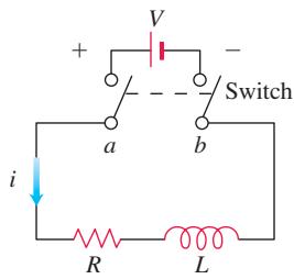
FIGURE 16.9 The RL circuit in Example 4.

教材插图

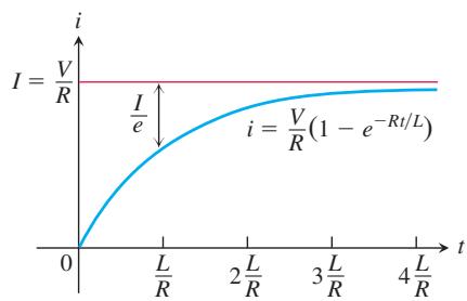
FIGURE 16.10 The growth of the current in the RL circuit in Example 4. I is the current’s steady-state value. The number $𝑡 = 𝐿 / 𝑅$ is the time constant of the circuit. The current gets to within 5% of its steady-state value in 3 time constants (Exercise 27).

RL Circuits

The diagram in Figure 16.9 represents an electrical circuit whose total resistance is a constant R ohms and whose self-inductance, shown as a coil, is L henries, also a constant. There is a switch whose terminals at a and b can be closed to connect a constant electrical source of V volts.

Ohm’s Law, $𝑉 : = : 𝑅 𝐼$ , has to be augmented for such a circuit. The correct equation accounting for both resistance and inductance is

𝐿 𝑑 𝑖 𝑑 𝑡 + 𝑅 𝑖 = 𝑉, (5)

where i is the current in amperes and t is the time in seconds. By solving this equation, we can predict how the current will flow after the switch is closed.

EXAMPLE 4 The switch in the RL circuit in Figure 16.9 is closed at time $𝑡 = 0$ . How will the current flow as a function of time?

Solution Equation (5) is a first-order linear differential equation for i as a function of t. Its standard form is

𝑑 𝑖 𝑑 𝑡 + 𝑅 𝐿 𝑖 = 𝑉 𝐿, (6)

and the corresponding solution, given that $𝑖 = 0$ when $𝑡 = 0$ , is

𝑖 = 𝑉 𝑅 - 𝑉 𝑅 𝑒 - (𝑅 / 𝐿) 𝑡 . (7)

(We leave the calculation of the solution to Exercise 28.) Since R and L are positive, $- (𝑅 / 𝐿)$ is negative and $𝑒 - (𝑅 / 𝐿) 𝑡 \to 0 a s 𝑡 \to \infty$ . Thus,

l i m 𝑡 \to \infty 𝑖 = l i m 𝑡 \to \infty (𝑉 𝑅 - 𝑉 𝑅 𝑒 - (𝑅 / 𝐿) 𝑡) = 𝑉 𝑅 - 𝑉 𝑅 \cdot 0 = 𝑉 𝑅 .

At any given time, the current is less than $𝑉 / 𝑅,$ but as time passes, the current approaches the steady-state value $𝑉 / 𝑅 .$ . According to the equation

𝐿 𝑑 𝑖 𝑑 𝑡 + 𝑅 𝑖 = 𝑉,

$𝐼 = 𝑉 / 𝑅$ is the current that will flow in the circuit if either $𝐿 = 0$ (no inductance) or $𝑑 𝑖 / 𝑑 𝑡 = 0$ (steady current, i = constant) (Figure 16.10).

Equation (7) expresses the solution of Equation (6) as the sum of two terms: a steady-state solution $𝑉 / 𝑅$ and a transient solution $- (𝑉 / ¯ 𝑅) 𝑒 - (𝑅 / 𝐿) 𝑡$ that tends to zero as $𝑡 ⟶ \infty .$

EXERCISES 16.2

First-Order Linear Equations

Solve the differential equations in Exercises 1–14.

$𝑥 𝑑 𝑦 𝑑 𝑥 + 𝑦 = 𝑒 𝑥, 𝑥 > 0$
$𝑒 𝑥 𝑑 𝑦 𝑑 𝑥 + 2 𝑒 𝑥 𝑦 = 1$
$𝑥 𝑦' + 3 𝑦 = s i n 𝑥 𝑥 2, 𝑥 > 0$
y x y x x tan cos , 2 2 2 ′ + = − < < ( ) π π
$𝑥 𝑑 𝑦 𝑑 𝑥 + 2 𝑦 = 1 - 1 𝑥, 𝑥 > 0$
$(1 + 𝑥) 𝑦' + 𝑦 = \sqrt 𝑥$
$2 𝑦' = 𝑒 𝑥 / 2 + 𝑦$
$𝑒 2 𝑥 𝑦' + 2 𝑒 2 𝑥 𝑦 = 2 𝑥$
$𝑥 𝑦' - 𝑦 = 2 𝑥 l n 𝑥$
$𝑥 𝑑 𝑦 𝑑 𝑥 = c o s 𝑥 𝑥 - 2 𝑦, 𝑥 > 0$
$(𝑡 - 1) 3 𝑑 𝑠 𝑑 𝑡 + 4 (𝑡 - 1) 2 𝑠 = 𝑡 + 1, 𝑡 > 1$

ds 1 12. t 1( )+ dt s t 2 3 1 ( ) + = + + t 1 ² ( )+ t 1 > −

^drsin θ cos tan , 0 2 r + = < < ( ) θ θ θ π dθ
$t a n 𝜃 𝑑 𝑟 𝑑 𝜃 + 𝑟 = s i n 2 𝜃, 0 < 𝜃 < 𝜋 / 2$

Solving Initial Value Problems

Solve the initial value problems in Exercises 15–20.

$𝑑 𝑦 𝑑 𝑡 + 2 𝑦 = 3, 𝑦 (0) = 1$
$𝑡 𝑑 𝑦 𝑑 𝑡 + 2 𝑦 = 𝑡 3, 𝑡 > 0, 𝑦 (2) = 1$
$𝜃 𝑑 𝑦 𝑑 𝜃 + 𝑦 = s i n 𝜃, 𝜃 > 0, 𝑦 (𝜋 / 2) = 1$
^dyθ 2 sec tan , 0, 3 2y y3 − = > =θ θ θ θ π( ) dθ
$(𝑥 + 1) 𝑑 𝑦 𝑑 𝑥 - 2 (𝑥 2 + 𝑥) 𝑦 = 𝑒 𝑥 2 𝑥 + 1, 𝑥 > - 1, 𝑦 (0) = 5$
$𝑑 𝑦 𝑑 𝑥 + 𝑥 𝑦 = 𝑥, 𝑦 (0) = - 6$
Solve the exponential growth/decay initial value problem for y as a function of t by thinking of the differential equation as a firstorder linear equation with $𝑃 (𝑥) = - 𝑘 a n d 𝑄 (𝑥) = 0;$

𝑑 𝑦 𝑑 𝑡 = 𝑘 𝑦 (𝑘 c o n s t a n t), 𝑦 (0) = 𝑦 0

Solve the following initial value problem for u as a function of t: $𝑑 𝑢 𝑑 𝑡 + 𝑘 𝑚 𝑢 = 0$ k m ( and positive constants), $𝑢 (0) = 𝑢 0$

a. as a first-order linear equation.

b. as a separable equation.

Theory and Examples

Is either of the following equations correct? Give reasons for your answers.

a. $𝑥 \int 1 𝑥 𝑑 𝑥 = 𝑥 l n | 𝑥 | + 𝐶$

b. $𝑥 \int 1 𝑥 𝑑 𝑥 = 𝑥 l n | 𝑥 | + 𝐶 𝑥$

Is either of the following equations correct? Give reasons for your answers.

a. $1 c o s 𝑥 \int c o s 𝑥 𝑑 𝑥 = t a n 𝑥 + 𝐶$

b. $1 c o s 𝑥 \int c o s 𝑥 𝑑 𝑥 = t a n 𝑥 + 𝐶 c o s 𝑥$

Current in a closed RL circuit How many seconds after the switch in an RL circuit is closed will it take the current i to reach half of its steady-state value? Notice that the time depends on R and $𝐿,$ not on how much voltage is applied.
Current in an open RL circuit If the switch is thrown open after the current in an RL circuit has built up to its steady-state value $𝐼 = 𝑉 / 𝑅$ , the decaying current (see accompanying figure) obeys the equation

𝐿 𝑑 𝑖 𝑑 𝑡 + 𝑅 𝑖 = 0,

which is Equation (5) with $𝑉 = 0$

a. Solve the equation to express i as a function of t.

b. How long after the switch is thrown will it take the current to fall to half its original value?

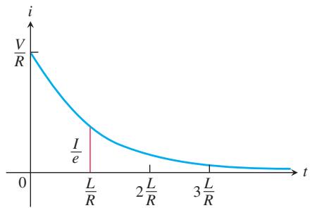
c. Show that the value of the current when $𝑡 = 𝐿 / 𝑅$ is $𝐼 / 𝑒 .$ . (The significance of this time is explained in the next exercise.)

教材插图

Time constants Engineers call the number $𝐿 / 𝑅$ the time constant of the RL circuit in Figure 16.10. The significance of the time constant is that the current will reach 95% of its final value within 3 time constants of the time the switch is closed (Figure 16.10). Thus, the time constant gives a built-in measure of how rapidly an individual circuit will reach equilibrium.

a. Find the value of i in Equation (7) that corresponds to $𝑡 = 3 𝐿 / 𝑅$ , and show that it is about 95% of the steady-state value $𝐼 = 𝑉 / 𝑅$

b. Approximately what percentage of the steady-state current will be flowing in the circuit 2 time constants after the switch is closed (i.e., when $𝑡 = 2 𝐿 / 𝑅) ?$

Derivation of Equation (7) in Example 4

a. Show that the solution of the equation

𝑑 𝑖 𝑑 𝑡 + 𝑅 𝐿 𝑖 = 𝑉 𝐿

𝑖 = 𝑉 𝑅 + 𝐶 𝑒 - (𝑅 / 𝐿) 𝑡 .

b. Then use the initial condition $𝑖 (0) = 0$ to determine the value of C. This will complete the derivation of Equation (7).

c. Show that $𝑖 = 𝑉 / 𝑅$ is a solution of Equation (6) and that $𝑖 = 𝐶 𝑒 - (𝑅 / 𝐿) 𝑡$ satisfies the equation

𝑑 𝑖 𝑑 𝑡 + 𝑅 𝐿 𝑖 = 0 .

A Bernoulli differential equation is of the form

𝑑 𝑦 𝑑 𝑥 + 𝑃 (𝑥) 𝑦 = 𝑄 (𝑥) 𝑦 𝑛 .

Observe that, if $𝑛 = 0 o r 1$ , the Bernoulli equation is linear. For other values of $𝑛,$ the substitution $𝑢 : = : 𝑦 1 - 𝑛$ transforms the Bernoulli equation into the linear equation

𝑑 𝑢 𝑑 𝑥 + (1 - 𝑛) 𝑃 (𝑥) 𝑢 = (1 - 𝑛) 𝑄 (𝑥) .

HISTORICAL BIOGRAPHY

Jakob Bernoulli

(1654–1705)

Jakob Bernoulli was born in Switzerland and received his degree in 1671 after studying philosophy and theology at the request of his father and mathematics and astronomy against the will of his father. Working on problems in optics and mechanics, Bernoulli contributed to important developments in infinitesimal geometry and calculus.

To know more, visit the companion Website.

For example, in the equation

𝑑 𝑦 𝑑 𝑥 - 𝑦 = 𝑒 - 𝑥 𝑦 2,

we have $𝑛 = 2,$ so that $𝑢 = 𝑦 1 - 2 = 𝑦 - 1$ and

$𝑑 𝑢 / 𝑑 𝑥 = - 𝑦 - 2 𝑑 𝑦 / 𝑑 𝑥 .$ . Then

𝑑 𝑦 / 𝑑 𝑥 = - 𝑦 2 𝑑 𝑢 / 𝑑 𝑥 = - 𝑢 - 2 𝑑 𝑢 / 𝑑 𝑥 .

Substitution into the original equation gives

- 𝑢 - 2 𝑑 𝑢 𝑑 𝑥 - 𝑢 - 1 = 𝑒 - 𝑥 𝑢 - 2,

or, equivalently,

𝑑 𝑢 𝑑 𝑥 + 𝑢 = - 𝑒 - 𝑥 .

This last equation is linear in the (unknown) dependent variable u.

Solve the Bernoulli equations in Exercises 29–32.

𝟐 𝟗 . 𝑦' - 𝑦 = - 𝑦 2 𝟑 𝟎 . 𝑦' - 𝑦 = 𝑥 𝑦 2 𝟑 𝟏 . 𝑥 𝑦' + 𝑦 = 𝑦 - 2 𝟑 𝟐 . 𝑥 2 𝑦' + 2 𝑥 𝑦 = 𝑦 3

16.3 Applications

We now look at four applications of first-order differential equations. The first application analyzes an object moving along a straight line while subject to a force opposing its motion. The second is a model of population growth. The third application considers a curve or curves intersecting each curve in a second family of curves orthogonally (that is, at right angles). The final application analyzes chemical concentrations entering and leaving a container. The various models involve separable or linear first-order equations.

Motion with Resistance Proportional to Velocity

In some cases it is reasonable to assume that the resistance encountered by a moving object, such as a car coasting to a stop, is proportional to the object’s velocity. The faster the object moves, the more its forward progress is resisted by the air through which it passes. Picture the object as a mass m moving along a coordinate line with position function s and velocity υ at time t. From Newton’s second law of motion, the resisting force opposing the motion is

F o r c e = m a s s \times a c c e l e r a t i o n = 𝑚 𝑑 𝑣 𝑑 𝑡 .

If the resisting force is proportional to velocity, we have

𝑚 𝑑 𝑣 𝑑 𝑡 = - 𝑘 𝑣 o r 𝑑 𝑣 𝑑 𝑡 = - 𝑘 𝑚 𝑣 (𝑘 > 0) .

This is a separable differential equation representing exponential change. The solution to the equation with initial condition $𝜐 = 𝑣 0$ at $𝑡 = 0$ is (Section 7.2)

𝑣 = 𝑣 0 𝑒 - (𝑘 / 𝑚) 𝑡 . (1)

What can we learn from Equation (1)? For one thing, we can see that if m is something large, like the mass of a 20,000-ton ore boat in Lake Erie, it will take a long time for the velocity to approach zero (because t must be large in the exponent of the equation in order to make kt m large enough for υ to be small). We can learn even more if we integrate Equation (1) to find the position s as a function of time t.

Suppose that an object is coasting to a stop and the only force acting on it is a resistance proportional to its speed. How far will it coast? To find out, we start with Equation (1) and solve the initial value problem

𝑑 𝑠 𝑑 𝑡 = 𝑣 0 𝑒 - (𝑘 / 𝑚) 𝑡, 𝑠 (0) = 0 .

Integrating with respect to t gives

𝑠 = - 𝑣 0 𝑚 𝑘 𝑒 - (𝑘 / 𝑚) 𝑡 + 𝐶 .

Substituting $𝑠 = 0$ when $𝑡 = 0$ gives

0 = - 𝑣 0 𝑚 𝑘 + 𝐶 a n d 𝐶 = 𝑣 0 𝑚 𝑘 .

The body’s position at time t is therefore

𝑠 (𝑡) = - 𝑣 0 𝑚 𝑘 𝑒 - (𝑘 / 𝑚) 𝑡 + 𝑣 0 𝑚 𝑘 = 𝑣 0 𝑚 𝑘 (1 - 𝑒 - (𝑘 / 𝑚) 𝑡) . (2)

To find how far the body will coast, we find the limit of s( ) ast $𝑡 ⟶ \infty .$ . Since $- (𝑘 / 𝑚) < 0$ we know that $𝑒 - (𝑘 / 𝑚) 𝑡 ⟶ 0 a s 𝑡 ⟶ \infty .$ , so that

l i m 𝑡 \to \infty 𝑠 (𝑡) = l i m 𝑡 \to \infty 𝑣 0 𝑚 𝑘 (1 - 𝑒 - (𝑘 / 𝑚) 𝑡) = 𝑣 0 𝑚 𝑘 (1 - 0) = 𝑣 0 𝑚 𝑘 .

Thus,

D i s t a n c e c o a t e d = 𝑣 0 𝑚 𝑘 . (3)

The number $𝑣 0 𝑚 / 𝑘$ is only an upper bound (albeit a useful one). It is true to life in one respect, at least: If m is large, the body will coast a long way.

EXAMPLE 1 For a 90-kg ice skater, the k in Equation (1) is about 5 $k g / s .$ How long will it take the skater to coast from $3.3 m / s (11.88 k m / h)$ to 0.3 m/s? How far will the skater coast before coming to a complete stop?

Solution We answer the first question by solving Equation (1) for t:

33 𝑒 - 𝑡 / 18 = 0 . 3 E q . (1) w i t h 𝑘 = 5, 𝑒 - 𝑡 / 18 = 1 / 11 𝑚 = 90, 𝑣 0 = 3 . 3, 𝑣 = 0 . 3 - 𝑡 / 18 = l n (1 / 11) = - l n 11 𝑡 = 18 l n 11 \approx 43 s .

We answer the second question with Equation (3):

D i s t a n c e c o a s t e d = 𝑣 0 𝑚 𝑘 = 3.3 \cdot 90 5 = 5 9 . 4 m .

Inaccuracy of the Exponential Population Growth Model

In Section 7.2 we modeled population growth with the Law of Exponential Change:

𝑑 𝑃 𝑑 𝑡 = 𝑘 𝑃, 𝑃 (0) = 𝑃 0,

where P is the population at time $𝑡, 𝑘 > 0$ is a constant growth rate, and $𝑃 0$ is the size of the population at time $𝑡 : = : 0$ . In Section 7.2 we found the solution $\boldsymbol𝑃 =𝑃0\boldsymbol𝑒𝑘𝑡$ to this model.

To assess the model, notice that the exponential growth differential equation says that

𝑑 𝑃 / 𝑑 𝑡 𝑃 = 𝑘 (4)

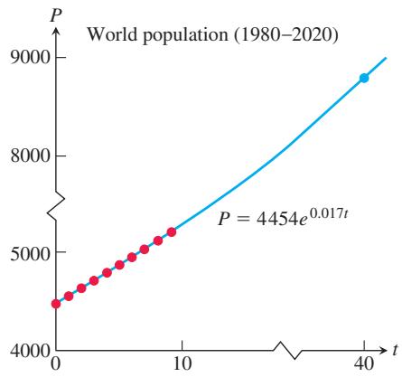
is constant. This rate is called the relative growth rate. We can use this to predict total future world population based on historical data. Table 16.3 gives the world population at midyear for the years 1980 to 19816. Taking $𝑑 𝑡 = 1$ and $𝑑 𝑃 \approx Δ 𝑃$ , we see from the table that the relative growth rate in Equation (4) is approximately equal to 0.017. Thus, based on the tabled data with $𝑡 = 0$ representing $1980, 𝑡 = 1$ representing 1981, and so forth, the world population could be modeled by the initial value problem

教材插图

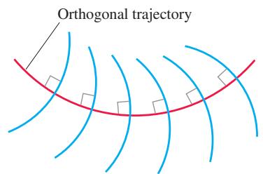
FIGURE 16.11 The value of the solution $𝑃 = 4454 𝑒 0.017 𝑡$ is 8792 when $𝑡 = 40,$ which is nearly 13% more than the actual population in 2020.

教材插图

FIGURE 16.12 An orthogonal trajectory intersects the family of curves at right angles, or orthogonally.

教材插图

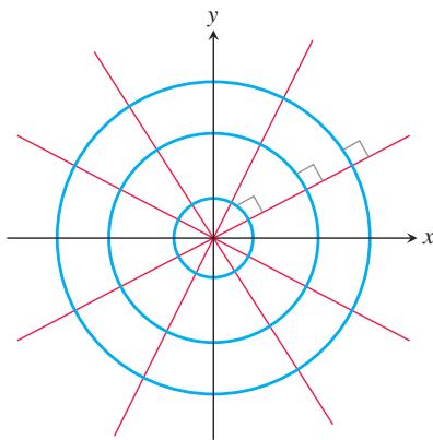
FIGURE 16.13 Every straight line through the origin is orthogonal to the family of circles centered at the origin.

TABLE 16.3 World population (midyear)

Year	Population (millions)	$Δ 𝑃 / 𝑃$
1980	4454	76/4454 ≈ 0.0171
1981	4530	80/4530 ≈ 0.0177
1982	4610	80/4610 ≈ 0.0174
1983	4690	80/4690 ≈ 0.0171
1984	4770	81/4770 ≈ 0.0170
1985	4851	82/4851 ≈ 0.0169
1986	4933	85/4933 ≈ 0.0172
1987	5018	87/5018 ≈ 0.0173
1988	5105	85/5105 ≈ 0.0167
1989	5190

𝑑 𝑃 𝑑 𝑡 = 0 . 017 𝑃, 𝑃 (0) = 445 4 .

The solution to this initial value problem gives the population function $𝑃 = 4454 𝑒 0.017 𝑡$ In year 2008 (so $𝑡 = 28)$ , the solution predicts the world population in midyear to be about 7169 million, or 7.2 billion (Figure 16.11), which is more than the actual population of 6707 million, an error of about 7%. The error grows as the number of years increases. For $2020 (𝑡 = 40)$ the model predicts a population of 8792 million. The reported population for 2020 is 7795 million, an overprediction error of about 13%. A more realistic model would consider environmental, economic, and other factors affecting the growth rate, which has been steadily declining. We consider one such model in Section 16.4.

Orthogonal Trajectories

An orthogonal trajectory of a family of curves is a curve that intersects each curve of the family at right angles, or orthogonally (Figure 16.12). For instance, each straight line through the origin is an orthogonal trajectory of the family of circles $𝑥 2 + 𝑦 2 = 𝑎 2$ , centered at the origin (Figure 16.13). Such mutually orthogonal systems of curves are of particular importance in physical problems related to electrical potential, where the curves in one family correspond to strength of an electric field, and those in the other family correspond to constant electric potential. They also occur in hydrodynamics and heat-flow problems.

EXAMPLE 2 Find the orthogonal trajectories of the family of curves $𝑥 𝑦 = 𝑎,$ , where $𝑎 \neq 0$ is an arbitrary constant.

Solution The curves xy a = form a family of hyperbolas having the coordinate axes as asymptotes. First we find the slopes of each curve in this family, or their $𝑑 𝑦 / 𝑑 𝑥$ values. Differentiating $𝑥 𝑦 = 𝑎$ implicitly gives

𝑥 𝑑 𝑦 𝑑 𝑥 + 𝑦 = 0 o r 𝑑 𝑦 𝑑 𝑥 = - 𝑦 𝑥 .

教材插图

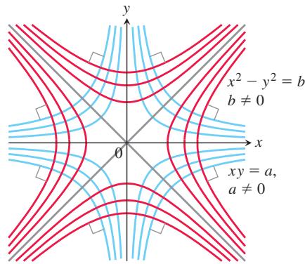
FIGURE 16.14 Each curve is orthogonal to every curve it meets in the other family (Example 2).

Thus the slope of the tangent line at any point $(𝑥, 𝑦)$ on one of the hyperbolas $𝑥 𝑦 = 𝑎$ is $𝑦' = - 𝑦 / 𝑥$ . On an orthogonal trajectory the slope of the tangent line at this same point must be the negative reciprocal, or $𝑥 / 𝑦$ . Therefore, the orthogonal trajectories must satisfy the differential equation

𝑑 𝑦 𝑑 𝑥 = 𝑥 𝑦 .

This differential equation is separable, and we solve it as in Section 7.2:

𝑦 𝑑 𝑦 = 𝑥 𝑑 𝑥 S e p a r a t e v a r i a b l e s . \int 𝑦 𝑑 𝑦 = \int 𝑥 𝑑 𝑥 I n t e g r a t e b o t h s i d e s . 12 𝑦 2 = 12 𝑥 2 + 𝐶 𝑦 2 - 𝑥 2 = 𝑏, (5)

where $𝑏 = 2 𝐶$ is an arbitrary constant. The orthogonal trajectories are the family of hyperbolas given by Equation (5) and sketched in Figure 16.14. ■

Mixture Problems

Suppose a chemical in a liquid solution (or dispersed in a gas) runs into a container holding the liquid (or the gas) with, possibly, a specified amount of the chemical dissolved as well. The mixture is kept uniform by stirring and flows out of the container at a known rate. In this process, it is often important to know the concentration of the chemical in the container at any given time. The differential equation describing the process is based on the formula

R a t e o f c h a n g e o f a m o u n t i n c o n t a i n e r = ⎛ ⎜ ⎜ ⎜ ⎜ ⎝ r a t e a t w h i c h c h e m i c a l a r r i v e s ⎞ ⎟ ⎟ ⎟ ⎟ ⎠ - ⎛ ⎜ ⎜ ⎜ ⎜ ⎝ r a t e a t w h i c h c h e m i c a l d e p a r t s . ⎞ ⎟ ⎟ ⎟ ⎟ ⎠ . (6)

If $𝑦 (𝑡)$ is the amount of chemical in the container at time t, and $𝑉 (𝑡)$ is the total volume of liquid in the container at time $𝑡,$ then the departure rate of the chemical at time t is

D e p a r t u r e r a t e = 𝑦 (𝑡) 𝑉 (𝑡) \cdot (o u t f l o w r a t e) = (c o n c e n t r a t i o n i n c o n t a i n e r a t t i m e 𝑡) \cdot (o u t f l o w r a t e) . (7)

Accordingly, Equation (6) becomes

𝑑 𝑦 𝑑 𝑡 = (c h e m i c a l' s a r r i v a l r a t e) - 𝑦 (𝑡) 𝑉 (𝑡) \cdot (o u t f l o w r a t e) . (8)

If, say, y is measured in kilograms, V in liters, and t in minutes, the units in Equation (8) are

k i l o g r a m s m i n u t e s = k i l o g r a m s m i n u t e s - k i l o g r a m s l i t e r s \cdot l i t e r s m i n u t e s .

EXAMPLE 3 In an oil refinery, a storage tank contains 10,000 L of gasoline that initially has 50 kg of an additive dissolved in it. In preparation for winter weather, gasoline containing 0.2 kg of additive per liter is pumped into the tank at a rate of 200 L/min.

The well-mixed solution is pumped out at a rate of 220 L/min. How much of the additive is in the tank 20 min after the pumping process begins (Figure 16.15)?

教材插图

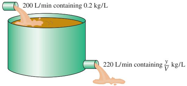
FIGURE 16.15 The storage tank in Example 3 mixes input

liquid with stored liquid to produce an output liquid.

Solution Let y be the amount (in kilograms) of additive in the tank at time t. We know that $𝑦 = 50$ when $𝑡 = 0$ . The number of liters of gasoline and additive in solution in the tank at any time t is

𝑉 (𝑡) = 10, 000 L + (200 L m i n - 220 L m i n) (𝑡 m i n) = (10, 000 - 20 𝑡) L .

Therefore,

R a t e o u t = 𝑦 (𝑡) 𝑉 (𝑡) \cdot o u t f l o w r a t e E q . (7) = (𝑦 10, 000 - 20 𝑡) 200 O u t f l o w r a t e i s 220 L / m i n = 220 𝑦 10, 000 - 20 𝑡 k g m i n . a n d V = 10, 000 - 20 t .

Also,

R a t e i n = (0 . 2 k g L) (200 L m i n) = 40 k g m i n .

The differential equation modeling the mixture process is

𝑑 𝑦 𝑑 𝑡 = 40 - 220 𝑦 10, 000 - 20 𝑡 E q . (8)

in kilograms per minute.

To solve this differential equation, we first write it in standard linear form:

𝑑 𝑦 𝑑 𝑡 + 220 10, 000 - 20 𝑡 𝑦 = 4 0 .

Thus, $𝑃 (𝑡) = 220 / (10, 000 - 20 𝑡)$ and $𝑄 (𝑡) = 40$ . The integrating factor is

𝑣 (𝑡) = 𝑒 \int 𝑃 𝑑 𝑡 = 𝑒 \int 220 10, 000 - 20 𝑡 𝑑 𝑡 = 𝑒 - 11 l n (10, 000 - 20 𝑡) 10, 000 - 20 𝑡 > 0 = (10, 000 - 20 𝑡) - 11 .

Multiplying both sides of the standard equation by υ( )t and integrating both sides gives

(10, 000 - 20 𝑡) - 11 \cdot (𝑑 𝑦 𝑑 𝑡 + 220 10, 000 - 20 𝑡 𝑦) = 40 (10, 000 - 20 𝑡) - 11

(10, 000 - 20 𝑡) - 11 𝑑 𝑦 𝑑 𝑡 + 220 (10, 000 - 20 𝑡) - 12 𝑦 = 40 (10, 000 - 20 𝑡) - 11

𝑑 𝑑 𝑡 [(10, 000 - 20 𝑡) - 11 𝑦] = 40 (10, 000 - 20 𝑡) - 11

(10, 000 - 20 𝑡) - 11 𝑦 = \int 40 (10, 000 - 20 𝑡) - 11 𝑑 𝑡

(10, 000 - 20 𝑡) - 11 𝑦 = 40 \cdot (10, 000 - 20 𝑡) - 10 (- 10) (- 20) + 𝐶 .

The general solution is

𝑦 = 0 . 2 (10, 000 - 20 𝑡) + 𝐶 (10, 000 - 20 𝑡) 11 .

Because $𝑦 = 50$ when t = 0, we can determine the value of C:

50 = 0 . 2 (10, 000 - 0) + 𝐶 (10, 000 - 0) 11

𝐶 = - 1950 (10, 000) 11 .

The particular solution of the initial value problem is

𝑦 = 0 . 2 (10, 000 - 20 𝑡) - 1950 (10, 000) 11 (10, 000 - 20 𝑡) 11 .

The amount of additive in the tank 20 min after the pumping begins is

𝑦 (20) = 0 . 2 [10, 000 - 20 (20)] - 1950 (10, 000) 11 [10, 000 - 20 (20)] 11 \approx 675 k g .

EXERCISES 16.3

Motion Along a Line

Coasting bicycle A 66-kg cyclist on a 7-kg bicycle starts coasting on level ground at 9 m s. The k in Equation (1) is about $3.9 k g / s$

a. About how far will the cyclist coast before reaching a complete stop?

b. How long will it take the cyclist’s speed to drop to 1 $m / s ?$

Coasting battleship An Iowa class battleship has mass around 51,000 metric tons (51,000,000 kg) and a k value in Equation (1) of about 59, 000 kg s. Assume that the ship loses power when it is moving at a speed of 9 m s.

a. About how far will the ship coast before it is dead in the water?

b. About how long will it take the ship’s speed to drop to 1 m s?

The data in Table 16.4 were collected with a motion detector and a CBL™ by Valerie Sharritts, then a mathematics teacher at St. Francis DeSales High School in Columbus, Ohio. The table shows the distance s (meters) coasted on inline skates in t s by her daughter Ashley when she was 10 years old. Find a model for Ashley’s position given by the data in Table 16.4 in the form of

TABLE 16.4 Ashley Sharritts skating data

t (s)	s (m)	t (s)	s (m)	t (s)	s (m)
0	0	2.24	3.05	4.48	4.77
0.16	0.31	2.40	3.22	4.64	4.82
0.32	0.57	2.56	3.38	4.80	4.84
0.48	0.80	2.72	3.52	4.96	4.86
0.64	1.05	2.88	3.67	5.12	4.88
0.80	1.28	3.04	3.82	5.28	4.89
0.96	1.50	3.20	3.96	5.44	4.90
1.12	1.72	3.36	4.08	5.60	4.90
1.28	1.93	3.52	4.18	5.76	4.91
1.44	2.09	3.68	4.31	5.92	4.90
1.60	2.30	3.84	4.41	6.08	4.91
1.76	2.53	4.00	4.52	6.24	4.90
1.92	2.73	4.16	4.63	6.40	4.91
2.08	2.89	4.32	4.69	6.56	4.91

Equation (2). Her initial velocity was $𝑣 0 = 2.75 m / s .$ , her mass $𝑚 = 39.921$ kg, and her total coasting distance was 4.91 m.

Coasting to a stop Table 16.5 shows the distance s (meters) coasted on inline skates in terms of time t (seconds) by Kelly Schmitzer. Find a model for her position in the form of Equation (2). Her initial velocity was $𝑣 0 = 0.80 m / s$ , her mass $𝑚 = 49.90 k g .$ and her total coasting distance was 1.32 m.

TABLE 16.5 Kelly Schmitzer skating data

t (s)	s (m)	t (s)	s (m)	t (s)	s (m)
0	0	1.5	0.89	3.1	1.30
0.1	0.07	1.7	0.97	3.3	1.31
0.3	0.22	1.9	1.05	3.5	1.32
0.5	0.36	2.1	1.11	3.7	1.32
0.7	0.49	2.3	1.17	3.9	1.32
0.9	0.60	2.5	1.22	4.1	1.32
1.1	0.71	2.7	1.25	4.3	1.32
1.3	0.81	2.9	1.28	4.5	1.32

Orthogonal Trajectories

In Exercises 5–10, find the orthogonal trajectories of the family of curves. Sketch several members of each family.

𝑦 = 𝑚 𝑥

𝑦 = 𝑐 𝑥 2

$2 𝑥 2 + 𝑦 2 = 𝑐 2$ $9 . 𝑦 = 𝑐 𝑒 - 𝑥$ 10. $𝑦 = 𝑒 𝑘 𝑥$
Show that the curves $2 𝑥 2 + 3 𝑦 2 = 5$ and $𝑦 2 = 𝑥 3$ are orthogonal.
Find the family of solutions of the given differential equation and the family of orthogonal trajectories. Sketch both families.

a. $𝑥 𝑑 𝑥 + 𝑦 𝑑 𝑦 = 0$

b. $𝑥 𝑑 𝑦 - 2 𝑦 𝑑 𝑥 = 0$

Mixture Problems

Salt mixture A tank initially contains 400 L of brine in which 20 kg/L of salt are dissolved. A brine containing 0.2 kg/L of salt runs into the tank at the rate of 20 L/min. The mixture is kept uniform by stirring and flows out of the tank at the rate of $16 L / m i n .$

a. At what rate (kilograms per minute) does salt enter the tank at time t?

b. What is the volume of brine in the tank at time t?

c. At what rate (kilograms per minute) does salt leave the tank at time t?

d. Write down and solve the initial value problem describing the mixing process.

e. Find the concentration of salt in the tank 25 min after the process starts.

Mixture problem A 800-L tank is half full of distilled water. At time t = 0, a solution containing 50 grams/L of concentrate enters the tank at the rate of 20 L/min, and the well-stirred mixture is withdrawn at the rate of 12 L/min.

a. At what time will the tank be full?

b. At the time the tank is full, how many kilograms of concentrate will it contain?

Fertilizer mixture A tank contains 400 L of fresh water. A solution containing 0.1 kg/L of soluble lawn fertilizer runs into the tank at the rate of 4 L/min, and the mixture is pumped out of the tank at the rate of 12 L/min. Find the maximum amount of fertilizer in the tank and the time required to reach the maximum.
Carbon monoxide pollution An executive conference room of a corporation contains 120 m ³ of air initially free of carbon monoxide. Starting at time t = 0, cigarette smoke containing 4% carbon monoxide is blown into the room at the rate of 0.008 m min ³ . A ceiling fan keeps the air in the room well circulated and the air leaves the room at the same rate of 0.008 m min³ . Find the time when the concentration of carbon monoxide in the room reaches 0.01%.

16.4 Graphical Solutions of Autonomous Equations

In Chapter 4 we learned that the sign of the first derivative tells where the graph of a function is increasing and where it is decreasing. The sign of the second derivative tells the concavity of the graph. We can build on our knowledge of how derivatives determine the shape of a graph to solve differential equations graphically. We will see that the ability to discern physical behavior from graphs is a powerful tool in understanding real-world systems. The starting ideas for a graphical solution are the notions of phase line and equilibrium value. We arrive at these notions by investigating, from a point of view quite different from that studied in Chapter 4, what happens when the derivative of a differentiable function is zero.

Equilibrium Values and Phase Lines

When we differentiate implicitly the equation

15 l n (5 𝑦 - 15) = 𝑥 + 1,

we obtain

15 (5 5 𝑦 - 15) 𝑑 𝑦 𝑑 𝑥 = 1 .

Solving for $𝑦' = 𝑑 𝑦 / 𝑑 𝑥 .$ , we find $𝑦' = 5 𝑦 - 15 = 5 (𝑦 - 3)$ . In this case the derivative $𝑦'$ is a function of y only (the dependent variable) and is zero when $𝑦 = 3$

A differential equation for which $𝑑 𝑦 / 𝑑 𝑥$ is a function of y only is called an autonomous differential equation. Let’s investigate what happens when the derivative in an autonomous equation equals zero. We assume any derivatives are continuous.

DEFINITION $I f 𝑑 𝑦 / 𝑑 𝑥 = 𝑔 (𝑦)$ is an autonomous differential equation, then the values of $𝑦$ for which $𝑑 𝑦 / 𝑑 𝑥 = 0$ are called equilibrium values or rest points.

Thus, equilibrium values are those at which no change occurs in the dependent variable, so y is at rest. The emphasis is on the value of y where $𝑑 𝑦 / 𝑑 𝑥 = 0$ , not the value of $𝑥,$ as we studied in Chapter 4. For example, the equilibrium values for the autonomous differential equation

𝑑 𝑦 𝑑 𝑥 = (𝑦 + 1) (𝑦 - 2)

are $𝑦 = - 1$ and $𝑦 = 2$

To construct a graphical solution to an autonomous differential equation, we first make a phase line for the equation, a plot on the y-axis that shows the equation’s equilibrium values along with the intervals where $𝑑 𝑦 / 𝑑 𝑥$ and $𝑑 2 𝑦 / 𝑑 𝑥 2$ are positive and negative. Then we know where the solutions are increasing and decreasing, and the concavity of the solution curves. These are the essential features we found in Section 4.4, so we can determine the shapes of the solution curves without having to find formulas for them.

EXAMPLE 1 Draw a phase line for the equation

𝑑 𝑦 𝑑 𝑥 = (𝑦 + 1) (𝑦 - 2),

and use it to sketch solutions to the equation.

Solution

Draw a number line for y and mark the equilibrium values $𝑦 = - 1 𝑎 𝑛 𝑑 𝑦 = 2 .$ where $𝑑 𝑦 / 𝑑 𝑥 = 0$

教材插图

Identify and label the intervals where $𝑦' > 0$ and $𝑦' < 0$ . This step resembles what we did in Section 4.3, only now we are marking the y-axis instead of the x-axis.

教材插图

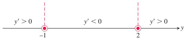
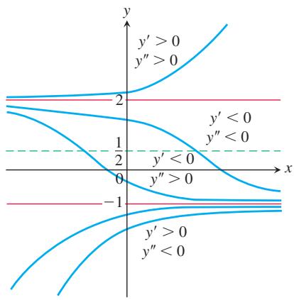
We can encapsulate the information about the sign of $𝑦'$ on the phase line itself. Since $𝑦' > 0$ on the interval to the left of $𝑦 = - 1$ , a solution of the differential equation with a y-value less than −1 will increase from there toward $𝑦 = - 1$ . We display this information by drawing an arrow on the interval pointing to −1.

教材插图

FIGURE 16.16 Graphical solutions from Example 1 include the horizontal lines $𝑦 = - 1$ and $𝑦 = 2$ through the equilibrium values. No two solution curves can ever cross or touch each other.

教材插图

Similarly, $𝑦' < 0$ between $𝑦 = - 1$ and $𝑦 = 2 .$ , so any solution with a value in this interval will decrease toward $𝑦 = - 1$

For $𝑦 > 2,$ we have $𝑦' > 0,$ , so a solution with a y-value greater than 2 will increase from there without bound.

In short, solution curves below the horizontal line $𝑦 = - 1$ in the xy-plane rise toward $𝑦 = - 1$ . Solution curves between the lines $𝑦 = - 1$ and $𝑦 = 2$ fall away from $𝑦 = 2$ toward $𝑦 = - 1$ . Solution curves above $𝑦 = 2$ rise away from $𝑦 = 2$ and keep going up.

Calculate $𝑦''$ and mark the intervals where $𝑦'' > 0$ and $𝑦'' < 0$ . To find $𝑦'',$ we differentiate $𝑦'$ with respect to x, using implicit differentiation.

教材插图

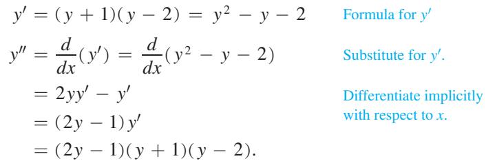
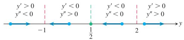
From this formula, we see that $𝑦''$ changes sign at $𝑦 = - 1, 𝑦 = 1 / 2$ , and $𝑦 = 2$ . We add the sign information to the phase line.

教材插图

Sketch an assortment of solution curves in the xy-plane. The horizontal lines $𝑦 = - 1, 𝑦 = 1 / 2$ , and $𝑦 = 2$ partition the plane into horizontal bands in which we know the signs of $𝑦'$ and $𝑦'' .$ . In each band, this information tells us whether the solution curves rise or fall and how they bend as x increases (Figure 16.16).

The “equilibrium lines” $𝑦 = - 1$ and $𝑦 = 2$ are also solution curves. (The constant functions $𝑦 = - 1$ and $𝑦 = 2$ satisfy the differential equation.) Solution curves that cross the line $𝑦 = 1 / 2$ have an inflection point there. The concavity changes from concave down (above the line) to concave up (below the line).

As predicted in Step 2, solutions in the middle and lower bands approach the equilibrium value $𝑦 = - 1$ as x increases. Solutions in the upper band rise steadily away from the value $𝑦 = 2$

Stable and Unstable Equilibria

Look at Figure 16.16 once more, in particular at the behavior of the solution curves near the equilibrium values. Once a solution curve has a value near $𝑦 = - 1,$ it tends steadily toward that value; $𝑦 = - 1$ is a stable equilibrium. The behavior near $𝑦 = 2$ is just the opposite: All solutions except the equilibrium solution $𝑦 = 2$ itself move away from it as x increases. We call $𝑦 = 2$ an unstable equilibrium. If the solution is at that value, it stays, but if it is off by any amount, no matter how small, it moves away. (Sometimes an equilibrium value is unstable because a solution moves away from it only on one side of the point.)

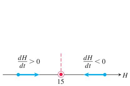
Now that we know what to look for, we can already see this behavior on the initial phase line (the second diagram in Step 2 of Example 1). The arrows lead away from $𝑦 = 2$ and, once to the left of $𝑦 = 2,$ , toward $𝑦 = - 1$

教材插图

FIGURE 16.17 First step in constructing the phase line for Newton’s Law of Cooling. The temperature tends toward the equilibrium (surrounding-medium) value in the long run.

教材插图

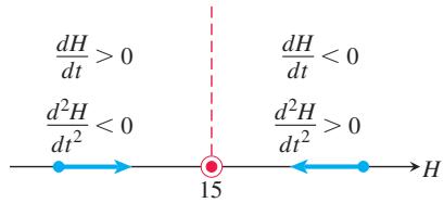
FIGURE 16.18 The complete phase line for Newton’s Law of Cooling.

教材插图

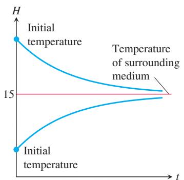
FIGURE 16.19 Temperature versus time. Regardless of initial temperature, the object’s temperature H t( ) tends toward $1 5 \circ C .$ , the temperature of the surrounding medium.

We now present several applied examples for which we can sketch a family of solution curves to the differential equation models using the method in Example 1.

Newton’s Law of Cooling

In Section 7.2 we solved analytically the differential equation

𝑑 𝐻 𝑑 𝑡 = - 𝑘 (𝐻 - 𝐻 𝑆), 𝑘 > 0

modeling Newton’s Law of Cooling. Here H is the temperature of an object at time t, and $𝐻 𝑠$ is the constant temperature of the surrounding medium.

Suppose that the surrounding medium (say, a room in a house) has a constant Celsius temperature of $1 5 \circ C$ . We can then express the difference in temperature as $𝐻 (𝑡) - 15$ Assuming H is a differentiable function of time t, by Newton’s Law of Cooling, there is a constant of proportionality $𝑘 > 0$ such that

𝑑 𝐻 𝑑 𝑡 = - 𝑘 (𝐻 - 15) (1)

(minus k to give a negative derivative when $𝐻 > 15)$ ).

Since $𝑑 𝐻 / 𝑑 𝑡 = 0$ at $𝐻 = 15,$ the temperature $1 5 \circ C$ is an equilibrium value. If $𝐻 > 15,$ Equation (1) tells us that $(𝐻 - 15) > 0$ and $𝑑 𝐻 / 𝑑 𝑡 < 0$ . If the object is hotter than the room, it will get cooler. Similarly, if $𝐻 < 15 .$ , then $(𝐻 - 15) < 0$ and $𝑑 𝐻 / 𝑑 𝑡 > 0$ An object cooler than the room will warm up. Thus, the behavior described by Equation (1) agrees with our intuition of how temperature should behave. These observations are captured in the initial phase line diagram in Figure 16.17. The value $𝐻 = 15$ is a stable equilibrium.

We determine the concavity of the solution curves by differentiating both sides of Equation (1) with respect to t:

𝑑 𝑑 𝑡 (𝑑 𝐻 𝑑 𝑡) = 𝑑 𝑑 𝑡 (- 𝑘 (𝐻 - 15)) 𝑑 2 𝐻 𝑑 𝑡 2 = - 𝑘 𝑑 𝐻 𝑑 𝑡 .

Since −k is negative, we see that $𝑑 2 𝐻 / 𝑑 𝑡 2$ is positive when $𝑑 𝐻 / 𝑑 𝑡 < 0$ and negative when $𝑑 𝐻 / 𝑑 𝑡 > 0$ . Figure 16.18 adds this information to the phase line.

The completed phase line shows that if the temperature of the object is above the equilibrium value of $1 5 \circ C$ , the graph of $𝐻 (𝑡)$ will be decreasing and concave upward. If the temperature is below $1 5 \circ C$ (the temperature of the surrounding medium), the graph of $𝐻 (𝑡)$ will be increasing and concave downward. We use this information to sketch typical solution curves (Figure 16.19).

From the upper solution curve in Figure 16.19, we see that as the object cools down, the rate at which it cools slows down because $𝑑 𝐻 / 𝑑 𝑡$ approaches zero. This observation is implicit in Newton’s Law of Cooling and contained in the differential equation, but the flattening of the graph as time advances gives an immediate visual representation of the phenomenon.

A Falling Body Encountering Resistance

Newton observed that the rate of change of the momentum of a moving object is equal to the net force applied to it. In mathematical terms,

𝐹 = 𝑑 𝑑 𝑡 (𝑚 𝑣), (2)

教材插图

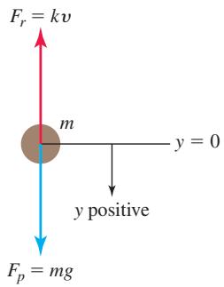
FIGURE 16.20 An object falling under the propulsion due to gravity, with a resistive force assumed to be proportional to the velocity.

教材插图

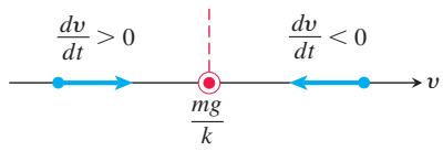
FIGURE 16.21 Initial phase line for the falling body encountering resistance.

教材插图

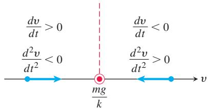
FIGURE 16.22 The completed phase line for the falling body.

教材插图

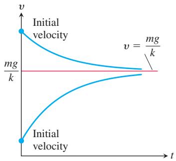
FIGURE 16.23 Typical velocity curves for a falling body encountering resistance. The value $𝜐 = 𝑚 𝑔 / 𝑘$ is the terminal velocity.

where $𝐹$ is the net force acting on the object, and m and υ are the object’s mass and velocity. If m varies with time, as it will if the object is a rocket burning fuel, the right-hand side of Equation (2) expands to

𝑚 𝑑 𝑣 𝑑 𝑡 + 𝑣 𝑑 𝑚 𝑑 𝑡

using the Derivative Product Rule. In many situations, however, m is constant, $𝑑 𝑚 / 𝑑 𝑡 = 0$ and Equation (2) takes the simpler form

𝐹 = 𝑚 𝑑 𝑣 𝑑 𝑡 o r 𝐹 = 𝑚 𝑎, (3)

which is known as Newton’s second law of motion (see Section 16.3).

In free fall, the constant acceleration due to gravity is denoted by $𝑔,$ and the one force propelling the body downward is

𝐹 𝑝 = 𝑚 𝑔,

the force due to gravity. If, however, we think of a real body falling through the air—say, a penny from a great height or a parachutist from an even greater height—we know that at some point air resistance is a factor in the speed of the fall. A more realistic model of free fall would include air resistance, shown as a force $𝐹 𝑟$ in the schematic diagram in Figure 16.20.

For low speeds well below the speed of sound, physical experiments have shown that $𝐹 𝑟$ is approximately proportional to the body’s velocity. The net force on the falling body is therefore

𝐹 = 𝐹 𝑝 - 𝐹 𝑟,

giving

𝑚 𝑑 𝑣 𝑑 𝑡 = 𝑚 𝑔 - 𝑘 𝑣 𝑑 𝑣 𝑑 𝑡 = 𝑔 - 𝑘 𝑚 𝑣 . (4)

We can use a phase line to analyze the velocity functions that solve this differential equation.

The equilibrium point, obtained by setting the right-hand side of Equation (4) equal to zero, is

𝑣 = 𝑚 𝑔 𝑘 .

If the body is initially moving faster than this, $𝑑 𝑣 / 𝑑 𝑡$ is negative and the body slows down. If the body is moving at a velocity below $𝑚 𝑔 / 𝑘$ , then $𝑑 𝑣 / 𝑑 𝑡 > 0$ and the body speeds up. These observations are captured in the initial phase line diagram in Figure 16.21.

We determine the concavity of the solution curves by differentiating both sides of Equation (4) with respect to t:

𝑑 2 𝑣 𝑑 𝑡 2 = 𝑑 𝑑 𝑡 (𝑔 - 𝑘 𝑚 𝑣) = - 𝑘 𝑚 𝑑 𝑣 𝑑 𝑡 .

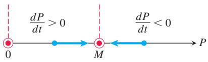
We see that $𝑑 2 𝑣 / 𝑑 𝑡 2 < 0$ when $𝜐 < 𝑚 𝑔 / 𝑘$ and that $𝑑 2 𝑣 / 𝑑 𝑡 2 > 0$ when $𝜐 > 𝑚 𝑔 / 𝑘 .$ Figure 16.22 adds this information to the phase line. Notice the similarity to the phase line for Newton’s Law of Cooling (Figure 16.18). The solution curves are similar as well (Figure 16.23).

教材插图

FIGURE 16.24 The initial phase line for logistic growth (Equation 6).

教材插图

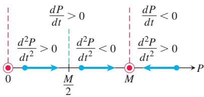
FIGURE 16.25 The completed phase line for logistic growth (Equation 6).

Figure 16.23 shows two typical solution curves. Regardless of the initial velocity, we see the body’s velocity tending toward the limiting value $𝜐 = 𝑚 𝑔 / 𝑘$ . This value, a stable equilibrium point, is called the body’s terminal velocity. Skydivers can vary their terminal velocity from 153 km/h to 290 km/h by changing the amount of body area opposing the fall, which affects the value of k.

The Logistic Model for Population Growth

In Section 16.3 we examined population growth using the model of exponential change. That is, if P represents the number of individuals and we neglect departures and arrivals, then

𝑑 𝑃 𝑑 𝑡 = 𝑘 𝑃, (5)

where $𝑘 > 0$ is the birth rate minus the death rate per individual per unit time.

Because the natural environment has only a limited number of resources to sustain life, it is reasonable to assume that only a maximum population M can be accommodated. As the population approaches this limiting population or carrying capacity, resources become less abundant and the growth rate k decreases. A simple relationship exhibiting this behavior is

𝑘 = 𝑟 (𝑀 - 𝑃),

where $𝑟 > 0$ is a constant. Notice that k decreases as P increases toward M and that k is negative if $𝑃$ is greater than M. Substituting $𝑟 (𝑀 - 𝑃)$ for k in Equation (5) gives the differential equation

𝑑 𝑃 𝑑 𝑡 = 𝑟 (𝑀 - 𝑃) 𝑃 = 𝑟 𝑀 𝑃 - 𝑟 𝑃 2 . (6)

The model given by Equation (6) is referred to as logistic growth.

We can forecast the behavior of the population over time by analyzing the phase line for Equation (6). The equilibrium values are $𝑃 = 𝑀$ and $𝑃 = 0$ , and we can see that $𝑑 𝑃 / 𝑑 𝑡 > 0 i f 0 < 𝑃 < 𝑀$ and $𝑑 𝑃 / 𝑑 𝑡 < 0 i f 𝑃 > 𝑀$ . These observations are recorded on the phase line in Figure 16.24.

We determine the concavity of the population curves by differentiating both sides of Equation (6) with respect to t:

𝑑 2 𝑃 𝑑 𝑡 2 = 𝑑 𝑑 𝑡 (𝑟 𝑀 𝑃 - 𝑟 𝑃 2) = 𝑟 𝑀 𝑑 𝑃 𝑑 𝑡 - 2 𝑟 𝑃 𝑑 𝑃 𝑑 𝑡 = 𝑟 (𝑀 - 2 𝑃) 𝑑 𝑃 𝑑 𝑡 . (7)

If $𝑃 = 𝑀 / 2$ , then $𝑑 2 𝑃 / 𝑑 𝑡 2 = 0 . I f 𝑃 < 𝑀 / 2$ , then $(𝑀 - 2 𝑃)$ and $𝑑 𝑃 / 𝑑 𝑡$ are positive and $𝑑 2 𝑃 / 𝑑 𝑡 2 > 0 . I f 𝑀 / 2 < 𝑃 < 𝑀$ , then $(𝑀 - 2 𝑃) < 0, 𝑑 𝑃 / 𝑑 𝑡 > 0$ , and $𝑑 2 𝑃 / 𝑑 𝑡 2 < 0$ . If $𝑃 > 𝑀$ , then $(𝑀 - 2 𝑃)$ and $𝑑 𝑃 / 𝑑 𝑡$ are both negative and $𝑑 2 𝑃 / 𝑑 𝑡 2 > 0$ . We add this information to the phase line (Figure 16.25).

The lines $𝑃 = 𝑀 / 2$ and $𝑃 = 𝑀$ divide the first quadrant of the tP-plane into horizontal bands in which we know the signs of both $𝑑 𝑃 / 𝑑 𝑡$ and $𝑑 2 𝑃 / 𝑑 𝑡 2$ . In each band, we know how the solution curves rise and fall, and how they bend as time passes. The equilibrium lines $𝑃 = 0$ and $𝑃 = 𝑀$ are both population curves. Population curves crossing the line

$𝑃 = 𝑀 / 2$ have an inflection point there, giving them a sigmoid shape (curved in two directions like a letter S). Figure 16.26 displays typical population curves. Notice that each population curve approaches the limiting population M as $𝑡 \infty$

教材插图

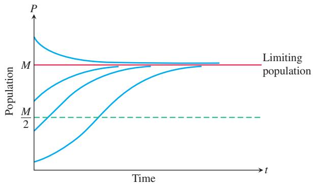
FIGURE 16.26 Population curves for logistic growth.

The Logistic Equation in Neural Networks and Machine Learning

While Figure 16.26 gives a general idea of the behavior of solutions to the Logistic Equation (6), we have not yet found explicit solutions. Exact formulas for solutions of first order differential equations cannot always be found, but they can be derived for the case of the Logistic Equation, where the solutions are called logistic functions. In Example 2 we find the solutions lying between $𝑦 = 0$ and $𝑦 = 1$ for the Logistic Equation in the case where $𝑀 = 1$ and r is an arbitrary positive constant.

EXAMPLE 2 Find the solutions to the Logistic Equation $𝑑 𝑦 𝑑 𝑥 = 𝑟 𝑦 - 𝑟 𝑦 2$ that satisfy $0\textless𝑦\textless1$ . Where does a solution cross the horizontal line $𝑦 = 1 / 2$ , and what is the slope of its graph at this point?

Solution To solve the differential equation we use the method of separation of variables introduced in Section 7.2.

𝑑 𝑦 𝑑 𝑥 = 𝑟 𝑦 - 𝑟 𝑦 2 = 𝑟 𝑦 (1 - 𝑦)

1 𝑦 (1 - 𝑦) 𝑑 𝑦 = 𝑟 𝑑 𝑥

\int 1 𝑦 (1 - 𝑦) 𝑑 𝑦 = \int 𝑟 𝑑 𝑥

\int 1 𝑦 + 1 1 - 𝑦 𝑑 𝑦 = \int 𝑟 𝑑 𝑥

Partial fractions

l n 𝑦 + 𝐶 1 - l n (1 - 𝑦) + 𝐶 2 = 𝑟 𝑥 + 𝐶 3

y y y y= − = −and 1 1 , since $0 < 𝑦 < 1$

l n 𝑦 - l n (1 - 𝑦) = 𝑟 𝑥 + 𝐶

Combine constants, $𝐶 = 𝐶 3 - 𝐶 1 - 𝐶 2$

l n 𝑦 1 - 𝑦 = 𝑟 𝑥 + 𝐶

𝑦 1 - 𝑦 = 𝑒 𝑟 𝑥 + 𝐶

Exponentiate.

𝑦 = 𝑒 𝑟 𝑥 + 𝐶 1 + 𝑒 𝑟 𝑥 + 𝐶

Use algebra to solve for y.

𝑦 = 1 1 + 𝑒 - 𝑟 𝑥 - 𝐶 .

Divide through by $𝑒 𝑟 𝑥 + 𝐶 .$

This gives an explicit formula for all the solutions whose graphs lie strictly between $𝑦 = 0$ and $𝑦 = 1$

When a solution crosses the line $𝑦 = 1 / 2$ we have

1 1 + 𝑒 - 𝑟 𝑥 - 𝐶 = 12 1 + 𝑒 - 𝑟 𝑥 - 𝐶 = 2 𝑒 - 𝑟 𝑥 - 𝐶 = 1 𝑟 𝑥 + 𝐶 = 0 𝑥 = - 𝐶 / 𝑟 .

So the solution graph crosses at the point $(- 𝐶 / 𝑟, 1 / 2)$ . The slope is found by evaluating $𝑑 𝑦 / 𝑑 𝑥 = 𝑟 𝑦 - 𝑟 𝑦 2$ at this point,

𝑑 𝑦 𝑑 𝑥 (- 𝐶 / 𝑟) = 𝑟 𝑦 - 𝑟 𝑦 2 = 𝑟 (1 / 2) - 𝑟 (1 / 2) 2 = 𝑟 4 .

Figure 16.27 shows the graph of a logistic function with $𝑟 = 3$ and $𝐶 = - 6$

教材插图

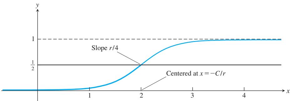
FIGURE 16.27 The constants r and C determine the steepness and horizontal displacement of a solution to the logistic equation. In this example $𝑟 = 3$ and $𝐶 = - 6$

Logistic functions have applications in many areas beyond the study of population growth. A field of Computer Science called Machine Learning develops methods to use a large collection of experimental data, called a training set, to construct a predictor function. The training set might consist of thousands of images of signs, for example, and the predictor function might decide whether a newly obtained image represents a Stop sign.

One highly successful approach to Machine Learning is the method of Neural Networks, which creates predictor functions based on a model of interacting neurons. Neural network models are built by taking repeated compositions of linear and logistic functions. Linear functions, such as $𝐿 (𝑥) = 𝑎 𝑥 + 𝑏$ can give accurate approximations of a function f nearby to a point where f is differentiable, as seen in Chapter 3. The optimal choices for the constants a and b in $𝐿 (𝑥)$ are found by minimizing an error function that is calculated using the training set in a process called linear regression. Logistic functions have several features that make them a useful complement to linear functions in constructing predictor functions. They have values lying between 0 and 1 and are well suited to modeling probabilities. They are differentiable and specified by a small number of constants, such as the constants r and C in Example 2. These constants can be adjusted, or tuned, to minimize the error of a prediction. Logistic functions are nonlinear, and taking compositions of linear and logistic functions allows for the approximation of much more complicated functions than linear functions alone. A more complete discussion of the utility of logistic functions involves multivariable functions and their derivatives, which are introduced in Chapter 13.

Exercises 16.4

Phase Lines and Solution Curves

In Exercises 1–8,

a. Identify the equilibrium values. Which are stable and which are unstable?

b. Construct a phase line. Identify the signs of y′ and $𝑦'' .$

c. Sketch several solution curves.

$𝑑 𝑦 𝑑 𝑥 = (𝑦 + 2) (𝑦 - 3) 𝟐 . 𝑑 𝑦 𝑑 𝑥 = 𝑦 2 - 4$
$𝑑 𝑦 𝑑 𝑥 = 𝑦 3 - 𝑦$
$𝑑 𝑦 𝑑 𝑥 = 𝑦 2 - 2 𝑦$
$𝑦' = \sqrt 𝑦, 𝑦 > 0$
$𝑦' = 𝑦 - \sqrt 𝑦, 𝑦 > 0$
$𝑦' = (𝑦 - 1) (𝑦 - 2) (𝑦 - 3) 8 . 𝑦' = 𝑦 3 - 𝑦 2$
$𝑑 𝑃 𝑑 𝑡 = 1 - 2 𝑃$
$𝑑 𝑃 𝑑 𝑡 = 𝑃 (1 - 2 𝑃)$
$𝑑 𝑃 𝑑 𝑡 = 2 𝑃 (𝑃 - 3)$
$𝑑 𝑃 𝑑 𝑡 = 3 𝑃 (1 - 𝑃) (𝑃 - 12)$
Catastrophic change in logistic growth Suppose that a healthy population of some species is growing in a limited environment and that the current population $𝑃 0$ is fairly close to the carrying capacity $𝑀 0 .$ You might imagine a population of fish living in a freshwater lake in a wilderness area. Suddenly a catastrophe such as the Mount St. Helens volcanic eruption contaminates the lake and destroys a significant part of the food and oxygen on which the fish depend. The result is a new environment with a carrying capacity $𝑀 1$ considerably less than $𝑀 0$ and, in fact, less than the current population $𝑃 0 .$ Starting at some time before the catastrophe, sketch a “before-and-after” curve that shows how the fish population responds to the change in environment.
Controlling a population The fish and game department in a certain state is planning to issue hunting permits to control the deer population (one deer per permit). It is known that if the deer population falls below a certain level m, the deer will become extinct. It is also known that if the deer population rises above the carrying capacity M, the population will decrease back to M through disease and malnutrition.

a. Discuss the reasonableness of the following model for the growth rate of the deer population as a function of time:

𝑑 𝑃 𝑑 𝑡 = 𝑟 𝑃 (𝑀 - 𝑃) (𝑃 - 𝑚),

where $𝑃$ is the population of the deer and r is a positive con stant of proportionality. Include a phase line.

b. Explain how this model differs from the logistic model $𝑑 𝑃 / 𝑑 𝑡 = 𝑟 𝑃 (𝑀 - 𝑃)$ . Is it more or less reasonable than the logistic model?

c. Show that if $𝑃 > 𝑀$ for all t, then lim $𝑃 (𝑡) = 𝑀 .$

d. What happens if $𝑃 <$ m for all t?

e. Discuss the solutions to the differential equation. What are the equilibrium points of the model? Explain the dependence of the steady-state value of P on the initial values of P. About how many permits should be issued?

Applications and Examples

Skydiving If a body of mass m falling from rest under the action of gravity encounters an air resistance proportional to the square of velocity, then the body’s velocity t seconds into the fall satisfies the equation

𝑚 𝑑 𝑣 𝑑 𝑡 = 𝑚 𝑔 - 𝑘 𝑣 2, 𝑘 > 0,

where k is a constant that depends on the body’s aerodynamic properties and the density of the air. (We assume that the fall is too short to be affected by changes in the air’s density.)

a. Draw a phase line for the equation.

b. Sketch a typical velocity curve.

c. For a 45-kg skydiver $(𝑚 𝑔 = 441)$ ) and with time in seconds and distance in meter, a typical value of k is 0.15. What is the diver’s terminal velocity? Repeat for an 80-kg skydiver.

Models of Population Growth

The autonomous differential equations in Exercises 16–12 represent models for population growth. For each exercise, use a phase line analysis to sketch solution curves for $𝑃 (𝑡),$ selecting different starting values P(0). Which equilibria are stable, and which are unstable?

Resistance proportional to $\sqrt 𝑣$ A body of mass m is projected vertically downward with initial velocity $𝑣 0 .$ Assume that the resisting force is proportional to the square root of the velocity, and find the terminal velocity from a graphical analysis.
Sailing A sailboat is running along a straight course with the wind providing a constant forward force of 200 N. The only other force acting on the boat is resistance as the boat moves through the water. The resisting force is numerically equal to five times the boat’s speed, and the initial velocity is $1 m / s .$ What is the maximum velocity in meters per second of the boat under this wind?
The spread of information Sociologists recognize a phenomenon called social diffusion, which is the spreading of a piece of information, technological innovation, or cultural fad among a population. The members of the population can be divided into two classes: those who have the information and those who do not. In a fixed population whose size is known, it is reasonable to assume that the rate of diffusion is proportional to the number who have the information times the number yet to receive it. If X denotes the number of individuals who have the information in a population of N people, then a mathematical model for social diffusion is given by

𝑑 𝑋 𝑑 𝑡 = 𝑘 𝑋 (𝑁 - 𝑋),

where t represents time in days and k is a positive constant.

a. Discuss the reasonableness of the model.

b. Construct a phase line identifying the signs of $𝑋'$ and $𝑋'' .$

c. Sketch representative solution curves.

d. Predict the value of X for which the information is spreading most rapidly. How many people eventually receive the information?

Current in an RL circuit The accompanying diagram represents an electrical circuit whose total resistance is a constant R ohms and whose self-inductance, shown as a coil, is L henries, also a constant. There is a switch whose terminals at a and b can be closed to connect a constant electrical source of V volts. From Section 16.2, we have

𝐿 𝑑 𝑖 𝑑 𝑡 + 𝑅 𝑖 = 𝑉,

where i is the current in amperes and t is the time in seconds.

教材插图

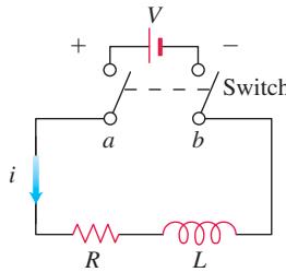
Use a phase line analysis to sketch the solution curve assuming that the switch in the RL circuit is closed at time $𝑡 = 0$ . What happens to the current as $𝑡 \infty ?$ This value is called the steadystate solution.

A pearl in shampoo Suppose that a pearl is sinking in a thick fluid, like shampoo, subject to a frictional force opposing its fall and proportional to its velocity. Suppose that there is also a resistive buoyant force exerted by the shampoo. According to Archimedes’ principle, the buoyant force equals the weight of the fluid displaced by the pearl. Using m for the mass of the pearl and P for the mass of the shampoo displaced by the pearl as it descends, complete the following steps.

a. Draw a schematic diagram showing the forces acting on the pearl as it sinks, as in Figure 16.20.

b. Using υ( )t for the pearl’s velocity as a function of time t, write a differential equation modeling the velocity of the pearl as a falling body.

c. Construct a phase line displaying the signs of $𝑣'$ and $𝑣'' .$

d. Sketch typical solution curves.

e. What is the terminal velocity of the pearl?

Logistic Functions

Write the formula for a logistic function that has values between $𝑦 = 0$ and $𝑦 = 1,$ , crosses the line $𝑦 = 1 / 2$ at $𝑥 = 0 .$ , and has slope 5 at this point.
Write the formula for a logistic function that has values between $𝑦 = 0$ and $𝑦 = 1,$ , crosses the line $𝑦 = 1 / 2$ at $𝑥 = 0$ , and has slope $1 / 5$ at this point.

Systems of Equations and Phase Planes

In some situations we are led to consider not one, but several, first-order differential equations. Such a collection is called a system of differential equations. In this section we present an approach to understanding systems through a graphical procedure known as a phase-plane analysis. We present this analysis in the context of modeling the populations of trout and bass living in a common pond.

Phase Planes

A general system of two first-order differential equations may take the form

𝑑 𝑥 𝑑 𝑡 = 𝐹 (𝑥, 𝑦),

𝑑 𝑦 𝑑 𝑡 = 𝐺 (𝑥, 𝑦) .

In this system we often think of t as representing time and take $𝑥 (𝑡)$ and y t( ) to be two functions of t. Such a system of equations is called autonomous because $𝑑 𝑥 / 𝑑 𝑡$ and $𝑑 𝑦 / 𝑑 𝑡$ do not depend on the independent variable time t, but only on the dependent variables x and y. A solution of such a system consists of a pair of functions x( ) and t y t( ) that satisfies both of the differential equations simultaneously for every t over some time interval (finite or infinite).

We cannot look at just one of these equations in isolation to find solutions $𝑥 (𝑡)$ or y t( ) since each derivative depends on both x and y. To gain insight into the solutions, we look at both dependent variables together by plotting the points $(𝑥 (𝑡), 𝑦 (𝑡))$ in the xy-plane starting at some specified point. Therefore the solution functions define a solution curve through the specified point, called a trajectory of the system. The xy-plane itself, in which these trajectories reside, is referred to as the phase plane. Thus we consider both solutions together and study the behavior of all the solution trajectories in the phase plane. It can be proved that two trajectories can never cross or touch each other. (Solution trajectories are examples of parametric curves, which will be examined in detail in Chapter 9.)

A Competitive-Hunter Model

Imagine two species of fish, say trout and bass, competing for the same limited resources (such as food and oxygen) in a certain pond. We let x( ) represent the number of trout andt y t( ) the number of bass living in the pond at time t. In reality, x( ) and t y t( ) are always integer valued, but we will approximate them with real-valued differentiable functions. This allows us to apply the methods of differential equations.

Several factors affect the rates of change of these populations. As time passes, each species breeds, so we assume its population increases proportionally to its size. Taken by itself, this would lead to exponential growth in each of the two populations. However, there is a countervailing effect from the fact that the two species are in competition. A large number of bass tends to cause a decrease in the number of trout, and vice versa. Our model takes the size of this effect to be proportional to the frequency with which the two species interact, which in turn is proportional to xy, the product of the two populations. These considerations lead to the following model for the growth of the trout and bass in the pond:

𝑑 𝑥 𝑑 𝑡 = (𝑎 - 𝑏 𝑦) 𝑥, (1 a)

𝑑 𝑦 𝑑 𝑡 = (𝑚 - 𝑛 𝑥) 𝑦 . (1 b)

Here $𝑥 (𝑡)$ represents the trout population, $𝑦 (𝑡)$ the bass population, and $𝑎, 𝑏,$ m, n are positive constants. A solution of this system then consists of a pair of functions $𝑥 (𝑡)$ and y t( ) that give the population of each fish species at time t. Each equation in (1) contains both of the unknown functions x and y, so we are unable to solve them individually. Instead, we will use a graphical analysis to study the solution trajectories of this competitive-hunter model.

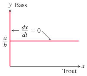
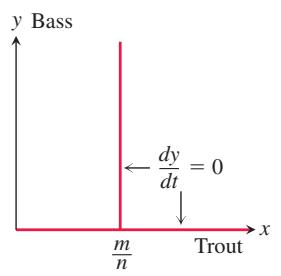
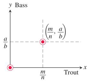
We now examine the nature of the phase plane in the trout-bass population model. We will be interested in the 1st quadrant of the xy-plane, where $𝑥 \geq 0$ and $𝑦 \geq 0$ , since populations cannot be negative. First, we determine where the bass and trout populations are both constant. Noting that the $(𝑥 (𝑡), 𝑦 (𝑡))$ values remain unchanged when $𝑑 𝑥 / 𝑑 𝑡 = 0$ and $𝑑 𝑦 / 𝑑 𝑡 = 0$ , we see that Equations (1a and 1b) then become

(𝑎 - 𝑏 𝑦) 𝑥 = 0, (𝑚 - 𝑛 𝑥) 𝑦 = 0 .

This pair of simultaneous equations has two solutions: $(𝑥, 𝑦) = (0, 0)$ and $(𝑥, 𝑦) = (𝑚 / 𝑛, 𝑎 / 𝑏)$ . At these $(𝑥, 𝑦)$ values, called equilibrium or rest points, the two populations remain at constant values over all time. The point (0, 0 represents a pond) containing no members of either fish species; the point $(𝑚 / 𝑛, 𝑎 / 𝑏)$ corresponds to a pond with an unchanging number of each fish species.

Next, we note that if $𝑦 = 𝑎 / 𝑏$ , then Equation (1a) implies $𝑑 𝑥 / 𝑑 𝑡 = 0$ , so the trout population x( ) is constant. Similarly, ift $𝑥 = 𝑚 / 𝑛$ , then Equation (1b) implies $𝑑 𝑦 / 𝑑 𝑡 = 0$ and the bass population y t( ) is constant. This information is recorded in Figure 16.28.

教材插图

(a)

教材插图

(b)

教材插图

(c)

FIGURE 16.28 Rest points in the competitive-hunter model given by Equations (1a) and (1b).

教材插图

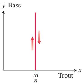
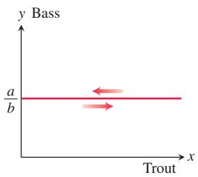
FIGURE 16.29 To the left of the line $𝑥 = 𝑚 / 𝑛$ the trajectories move upward, and to the right they move downward.

教材插图

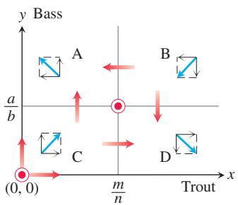
FIGURE 16.30 Above the line $𝑦 = 𝑎 / 𝑏$ the trajectories move to the left, and below it they move to the right.

教材插图

FIGURE 16.31 Composite graphical analysis of the trajectory directions in the four regions determined by $𝑥 = 𝑚 / 𝑛$ and $𝑦 = 𝑎 / 𝑏$

In setting up our competitive-hunter model, we do not generally know precise values of the constants a, b, m, n. Nonetheless, we can analyze the system of Equations (1) to learn the nature of its solution trajectories. We begin by determining the signs of $𝑑 𝑥 / 𝑑 𝑡$ and $𝑑 𝑦 / 𝑑 𝑡$ throughout the phase plane. Although $𝑥 (𝑡)$ represents the number of trout and $𝑦 (𝑡)$ the number of bass at time t, we are thinking of the pair of values $(𝑥 (𝑡), 𝑦 (𝑡))$ as a point tracing out a trajectory curve in the phase plane. When $𝑑 𝑥 / 𝑑 𝑡$ is positive, x( ) is increasingt and the point is moving to the right in the phase plane. If $𝑑 𝑥 / 𝑑 𝑡$ is negative, the point is moving to the left. Likewise, the point is moving upward where $𝑑 𝑦 / 𝑑 𝑡$ is positive and downward where $𝑑 𝑦 / 𝑑 𝑡$ is negative.

We saw that $𝑑 𝑦 / 𝑑 𝑡 = 0$ along the vertical line $𝑥 = 𝑚 / 𝑛$ . To the left of this line, $𝑑 𝑦 / 𝑑 𝑡$ is positive since $𝑑 𝑦 / 𝑑 𝑡 = (𝑚 - 𝑛 𝑥) .$ y and $𝑥 < 𝑚 / 𝑛$ . So the trajectories on this side of the line are directed upward. To the right of this line, $𝑑 𝑦 / 𝑑 𝑡$ is negative and the trajectories point downward. The directions of the associated trajectories are indicated in Figure 16.29. Similarly, above the horizontal line $𝑦 = 𝑎 / 𝑏$ , we have $𝑑 𝑥 / 𝑑 𝑡 < 0$ and the trajectories head leftward; below this line they head rightward, as shown in Figure 16.30. Combining this information gives four distinct regions in the plane $𝐴, 𝐵, 𝐶, 𝐷 i$ , with their respective trajectory directions shown in Figure 16.31.

Next, we examine what happens near the two equilibrium points. The trajectories near $(0, 0)$ point away from it, upward and to the right. The behavior near the equilibrium point $(𝑚 / 𝑛, 𝑎 / 𝑏)$ depends on the region in which a trajectory begins. If it starts in region $𝐵,$ for instance, then it will move downward and leftward toward the equilibrium point. Depending on where the trajectory begins, it may move downward into region $𝐷,$ leftward into region $𝐴,$ or perhaps straight into the equilibrium point. If it enters into regions A or $𝐷,$ then it will continue to move away from the rest point. We say that both rest points are unstable, meaning (in this setting) there are trajectories near each point that head away from them. These features are indicated in Figure 16.32.

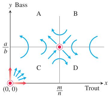
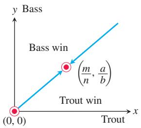
It turns out that in each of the half-planes above and below the line $𝑦 = 𝑎 / 𝑏$ , there is exactly one trajectory approaching the equilibrium point $(𝑚 / 𝑛, 𝑎 / 𝑏)$ (see Exercise $7)$ Above these two trajectories the bass population increases, and below them it decreases. The two trajectories approaching the equilibrium point are suggested in Figure 16.33.

教材插图

FIGURE 16.32 Motion along the trajectories near the rest points (0, 0) and $(𝑚 / 𝑛, 𝑎 / 𝑏)$ .

FIGURE 16.33 Qualitative results of analyzing the competitive-hunter model. There are exactly two trajectories approaching the point $(𝑚 / 𝑛, 𝑎 / 𝑏)$

Our graphical analysis leads us to conclude that, under the assumptions of the competitivehunter model, it is unlikely that both species will reach equilibrium levels. This is because it would be almost impossible for the fish populations to move exactly along one of the two approaching trajectories for all time. Furthermore, the initial populations point $(𝑥 0, 𝑦 0)$ determines which of the two species is likely to survive over time, and mutual coexistence of the species is highly improbable.

教材插图

Limitations of the Phase-Plane Analysis Method

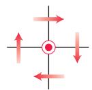
FIGURE 16.34 Trajectory direction near the rest point ( 0, 0 .)

Unlike the situation for the competitive-hunter model, it is not always possible to determine the behavior of trajectories near a rest point. For example, suppose we know that the trajectories near a rest point, chosen here to be the origin (0, 0 , behave as in Figure 16.34.) The information provided by Figure 16.34 is not sufficient to distinguish among the three possible trajectories shown in Figure 16.35. Even if we could determine that a trajectory near an equilibrium point resembles that of Figure 16.35c, we would still not know how the other trajectories behave. It could happen that a trajectory closer to the origin behaves like the motions displayed in Figure 16.35a or 16.35b. The spiraling trajectory in Figure 16.35c can never actually reach the rest point in a finite time period.

教材插图

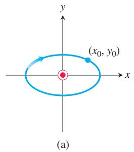
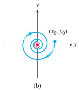
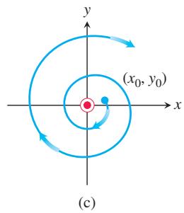
FIGURE 16.35 Three possible trajectory motions: (a) periodic motion, (b) motion toward an asymptotically stable rest point, and (c) motion near an unstable rest point.

Another Type of Behavior

教材插图

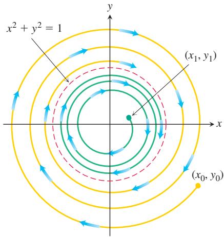
The system

𝑑 𝑥 𝑑 𝑡 = 𝑦 + 𝑥 - 𝑥 (𝑥 2 + 𝑦 2),

FIGURE 16.36 The solution $𝑥 2 + 𝑦 2 = 1$ is a limit cycle.

𝑑 𝑦 𝑑 𝑡 = - 𝑥 + 𝑦 - 𝑦 (𝑥 2 + 𝑦 2) (2 a)

(2b)

can be shown to have only one equilibrium point at (0, 0 . Yet any trajectory starting on the) unit circle traverses it clockwise because, when $𝑥 2 + 𝑦 2 = 1;$ , we have $𝑑 𝑦 / 𝑑 𝑥 = - 𝑥 / 𝑦$ (see Exercise 2). If a trajectory starts inside the unit circle, it spirals outward, asymptotically approaching the circle as $𝑡 \infty$ . If a trajectory starts outside the unit circle, it spirals inward, again asymptotically approaching the circle as $𝑡 \infty$ . The circle $𝑥 2 + 𝑦 2 = 1$ is called a limit cycle of the system (Figure 16.36). In this system, the values of x and y eventually become periodic.

Exercises 16.5

List three of the important considerations that are ignored in the competitive-hunter model as presented in the text.
For the system (2a) and (2b), show that any trajectory starting on the unit circle $𝑥 2 + 𝑦 2 = 1$ will traverse the unit circle in a periodic solution. First introduce polar coordinates and rewrite the system as $𝑑 𝑟 / 𝑑 𝑡 = 𝑟 (1 - 𝑟 2) a n d - 𝑑 𝜃 / 𝑑 𝑡 = - 1$
Develop a model for the growth of trout and bass, assuming that in isolation trout demonstrate exponential decay [so that $𝑎 < 0$ in Equations (1a) and (1b)] and that the bass population grows logistically with a population limit M. Analyze graphically the motion in the vicinity of the rest points in your model. Is coexistence possible?
How might the competitive-hunter model be validated? Include a discussion of how the various constants a, $𝑏, 𝑚,$ and n might be estimated. How could state conservation authorities use the model to ensure the survival of both species?
Consider another competitive-hunter model defined by

𝑑 𝑥 𝑑 𝑡 = 𝑎 (1 - 𝑥 𝑘 1) 𝑥 - 𝑏 𝑥 𝑦,

𝑑 𝑦 𝑑 𝑡 = 𝑚 (1 - 𝑦 𝑘 2) 𝑦 - 𝑛 𝑥 𝑦,

where x and y represent trout and bass populations, respectively.

a. What assumptions are implicitly being made about the growth of trout and bass in the absence of competition?

b. Interpret the constants a, b, m, $𝑛, 𝑘 1, 𝑘 2, 𝑎 / 𝑏$ , and m n in terms of the physical problem.

c. Perform a graphical analysis:

i) Find the possible equilibrium levels.

ii) Determine whether coexistence is possible.

iii) Pick several typical starting points, and sketch typical trajectories in the phase plane.

iv) Interpret the outcomes predicted by your graphical analysis in terms of the constants $𝑎, 𝑏, 𝑚, 𝑛, 𝑘 1$ , and $𝑘 2$

Note: When you get to part (iii), you should realize that five cases exist. You will need to analyze all five cases.

An economic model Consider the following economic model. Let P be the price of a single item on the market. Let $\boldsymbol𝑄$ be the quantity of the item available on the market. Both P and Q are functions of time. If one considers price and quantity as two interacting species, the following model might be proposed:

𝑑 𝑃 𝑑 𝑡 = 𝑎 𝑃 (𝑏 𝑄 - 𝑃), 𝑑 𝑄 𝑑 𝑡 = 𝑐 𝑄 (𝑓 𝑃 - 𝑄),

where $𝑎, 𝑏, 𝑐,$ and f are positive constants. Justify and discuss the adequacy of the model.

a. If $𝑎 = 1, 𝑏 = 20, 000, 𝑐 = 1,$ and $𝑓 = 30$ , find the equilibrium points of this system. If possible, classify each equilibrium point with respect to its stability. If a point cannot be readily classified, give some explanation.

b. Perform a graphical stability analysis to determine what will happen to the levels of P and Q as time increases.

c. Give an economic interpretation of the curves that determine the equilibrium points.

Two trajectories approach equilibrium Show that the two trajectories leading to $(𝑚 / 𝑛, 𝑎 / 𝑏)$ shown in Figure 16.33 are unique by carrying out the following steps.

a. From system (1a) and (1b) apply the Chain Rule to derive the following equation:

𝑑 𝑦 𝑑 𝑥 = (𝑚 - 𝑛 𝑥) 𝑦 (𝑎 - 𝑏 𝑦) 𝑥 .

b. Separate the variables, integrate, and exponentiate to obtain

𝑦 𝑎 𝑒 - 𝑏 𝑦 = 𝐾 𝑥 𝑚 𝑒 - 𝑛 𝑥,

where K is a constant of integration.

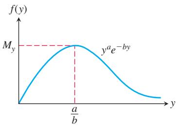
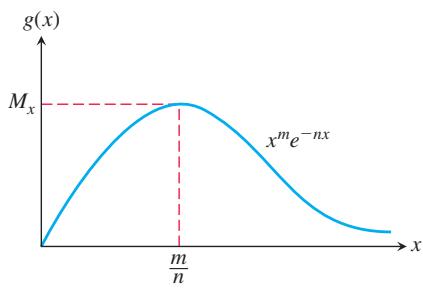
c. Let $𝑓 (𝑦) = 𝑦 𝑎 / 𝑒 𝑏 𝑦$ and $𝑔 (𝑥) = 𝑥 𝑚 / 𝑒 𝑛 𝑥$ . Show that $𝑓 (𝑦)$ has a unique maximum of $𝑀 v = (𝑎 / 𝑒 𝑏) 𝑎$ when $𝑦 = 𝑎 / 𝑏$ as shown in Figure 16.37. Similarly, show that g x( ) has a unique maximum $𝑀 𝑥 = (𝑚 / 𝑒 𝑛) 𝑚$ when $𝑥 = 𝑚 / 𝑛$ , also shown in Figure 16.37.

教材插图

FIGURE 16.37 Graphs of the functions $𝑓 (𝑦) = 𝑦 𝑎 / 𝑒 𝑏 𝑦$ and $𝑔 (𝑥) = 𝑥 𝑚 / 𝑒 𝑛 𝑥$

d. Consider what happens as $(𝑥, 𝑦)$ approaches $(𝑚 / 𝑛, 𝑎 / 𝑏)$ Take limits in part (b) as x → m n and $𝑦 𝑎 / 𝑏$ to show that either

l i m 𝑥 \to 𝑚 / 𝑛 𝑦 \to 𝑎 / 𝑏 [(𝑦 𝑎 𝑒 𝑏 𝑦) (𝑒 𝑛 𝑥 𝑥 𝑚)] = 𝐾

or $𝑀 𝑣 / 𝑀 𝑥 = 𝐾$ . Thus any solution trajectory that approaches $(𝑚 / 𝑛, 𝑎 / 𝑏)$ must satisfy)

𝑦 𝑎 𝑒 𝑏 𝑦 = (𝑀 𝑦 𝑀 𝑥) (𝑥 𝑚 𝑒 𝑛 𝑥) .

e. Show that only one trajectory can approach $(𝑚 / 𝑛, 𝑎 / 𝑏)$ from below the line $𝑦 = 𝑎 / 𝑏$ . Pick $𝑦 0 < 𝑎 / 𝑏$ . From Figure 16.37 you can see that $𝑓 (𝑦 0) < 𝑀 v$ , which implies that

𝑀 𝑦 𝑀 𝑥 (𝑥 𝑚 𝑒 𝑛 𝑥) = 𝑦 𝑎 0 / 𝑒 𝑏 𝑦 0 < 𝑀 𝑦 .

This in turn implies that

𝑥 𝑚 𝑒 𝑛 𝑥 < 𝑀 𝑥 .

Figure 16.37 tells you that for $𝑔 (𝑥)$ there is a unique value $𝑥 0 < 𝑚 / 𝑟$ n satisfying this last inequality. That is, for each $𝑦 < 𝑎 / 𝑏$ there is a unique value of x satisfying the equation in part (d). Thus there can exist only one trajectory solution approaching $(𝑚 / 𝑛, 𝑎 / 𝑏)$ from below, as shown in Figure 16.38.

f. Use a similar argument to show that the solution trajectory leading to $(𝑚 / 𝑛, 𝑎 / 𝑏)$ is unique if $𝑦 0 > 𝑎 / 𝑏$

教材插图

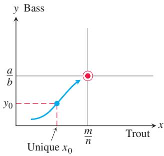
FIGURE 16.38 For any $𝑦 < 𝑎 / 𝑏$ , only one solution trajectory leads to the rest point $(𝑚 / 𝑛, 𝑎 / 𝑏)$

Show that the second-order differential equation $𝑦'' = 𝐹 (𝑥, 𝑦, 𝑦')$ can be reduced to a system of two first-order differential equations

𝑑 𝑦 𝑑 𝑥 = 𝑧, 𝑑 𝑧 𝑑 𝑥 = 𝐹 (𝑥, 𝑦, 𝑧) .

Can something similar be done to the nth-order differential equation $𝑦 (𝑛) = 𝐹 (𝑥, 𝑦, 𝑦', 𝑦'', \dots, 𝑦 (𝑛 - 1)) 𝑐$ 6

Lotka-Volterra Equations for a Predator-Prey Model

In 1925 Lotka and Volterra introduced the predator-prey equations, a system of equations that models the populations of two species, one of which preys on the other. Let x( ) represent the number of rabbitst living in a region at time t, and y t( ) the number of foxes in the same region. As time passes, the number of rabbits increases at a rate proportional to their population, and decreases at a rate proportional to the number of encounters between rabbits and foxes. The foxes, which compete for food, increase in number at a rate proportional to the number of encounters with rabbits but decrease at a rate proportional to the number of foxes. The number of encounters between rabbits and foxes is assumed to be proportional to the product of the two populations. These assumptions lead to the autonomous system

𝑑 𝑥 𝑑 𝑡 = (𝑎 - 𝑏 𝑦) 𝑥, 𝑑 𝑦 𝑑 𝑡 = (- 𝑐 + 𝑑 𝑥) 𝑦,

where $𝑎, 𝑏, 𝑐, 𝑑$ are positive constants. The values of these constants vary according to the specific situation being modeled. We can study the nature of the population changes without setting these constants to specific values.

What happens to the rabbit population if there are no foxes present?
What happens to the fox population if there are no rabbits present?
Show that (0, 0 and) $(𝑐 / 𝑑, 𝑎 / 𝑏)$ are equilibrium points. Explain the meaning of each of these points.
Show, by differentiating, that the function

𝐶 (𝑡) = 𝑎 l n 𝑦 (𝑡) - 𝑏 𝑦 (𝑡) - 𝑑 𝑥 (𝑡) + 𝑐 l n 𝑥 (𝑡)

is constant when x( ) and t y t( ) are positive and satisfy the predatorprey equations.

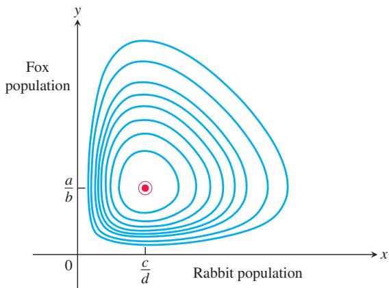
While x and y may change over time, C t( ) does not. Thus, C is a conserved quantity and its existence gives a conservation law. A trajectory that begins at a point ( , ) at timex y $𝑡 = 0$ gives a value of C that remains unchanged at future times. Each value of the constant C gives a trajectory for the autonomous system, and these trajectories close up, rather than spiraling inward or outward. The rabbit and fox populations oscillate through repeated cycles along a fixed trajectory. Figure 16.39 shows several trajectories for the predator-prey system.

教材插图

FIGURE 16.39 Some trajectories along which C is conserved.

Using a procedure similar to that in the text for the competitivehunter model, show that each trajectory is traversed in a counterclockwise direction as time t increases.

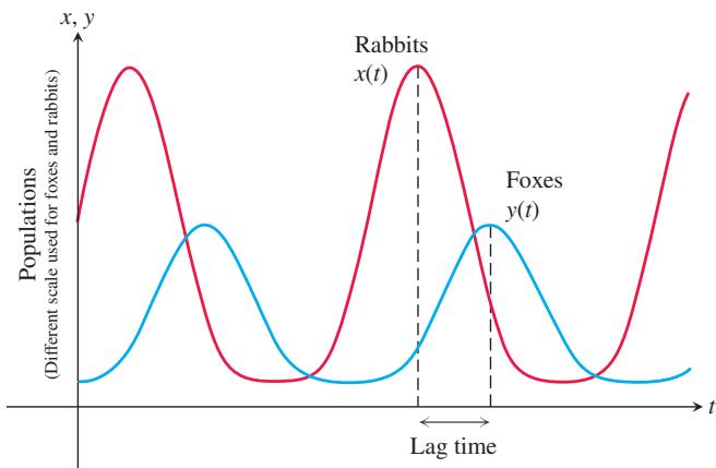
Along each trajectory, both the rabbit and fox populations fluctuate between their maximum and minimum levels. The maximum and minimum levels for the rabbit population occur where the trajectory intersects the horizontal line $𝑦 = 𝑎 / 𝑏$ . For the fox population, they occur where the trajectory intersects the vertical line $𝑥 = 𝑐 / 𝑑$ When the rabbit population is at its maximum, the fox population is below its maximum value. As the rabbit population declines from this point in time, we move counterclockwise around the trajectory, and the fox population grows until it reaches its maximum value. At this point the rabbit population has declined to $𝑥 = 𝑐 / 𝑑$ and is no longer at its peak value. We see that the fox population reaches its maximum value at a later time than the rabbits. The predator population lags behind that of the prey in achieving its maximum values. This lag effect is shown in Figure 16.40, which graphs both x( ) and t y t( ).

教材插图

FIGURE 16.40 The fox and rabbit populations oscillate periodically, with the maximum fox population lagging the maximum rabbit population.

CHAPTER 16 Questions to Guide Your Review

What is a first-order differential equation? When is a function a solution of such an equation?
At some time during a trajectory cycle, a wolf invades the rabbit– fox territory, eats some rabbits, and then leaves. Does this mean that the fox population will from then on have a lower maximum value? Explain your answer.
What is a general solution? What is a particular solution?
What is the slope field of a differential equation $𝑦' = 𝑓 (𝑥, 𝑦) ?$ What can we learn from such fields?
Describe Euler’s method for solving the initial value problem $𝑦' = 𝑓 (𝑥, 𝑦), 𝑦 (𝑥 0) = 𝑦 0$ numerically. Give an example. Comment on the method’s accuracy. Why might you want to solve an initial value problem numerically?
How do you solve linear first-order differential equations?
What is an orthogonal trajectory of a family of curves? Describe how one is found for a given family of curves.
What is an autonomous differential equation? What are its equilibrium values? How do they differ from critical points? What is a stable equilibrium value? Unstable?
How do you construct the phase line for an autonomous differential equation? How does the phase line help you produce a graph that qualitatively depicts a solution to the differential equation?
Why is the exponential model unrealistic for predicting long-term population growth? How does the logistic model correct for the deficiency in the exponential model for population growth? What is the logistic differential equation? What is the form of its solution? Describe the graph of the logistic solution.
What is an autonomous system of differential equations? What is a solution to such a system? What is a trajectory of the system?

CHAPTER 16 Practice Exercises

In Exercises 1–22, solve the differential equation.

$𝑦' = 𝑥 𝑒 𝑦 \sqrt 𝑥 - 2$
$𝑦' = 𝑥 𝑦 𝑒 𝑥 2$
$s e c 𝑥 𝑑 𝑦 + 𝑥 c o s 2 𝑦 𝑑 𝑥 = 0$
$2 𝑥 2 𝑑 𝑥 - 3 \sqrt 𝑦 c s c 𝑥 𝑑 𝑦 = 0$
$𝑦' = 𝑒 𝑦 𝑥 𝑦$
$𝑦' = 𝑥 𝑒 𝑥 - 𝑦 c s c 𝑦$
$𝑥 (𝑥 - 1) 𝑑 𝑦 - 𝑦 𝑑 𝑥 = 0$
$𝑦' = (𝑦 2 - 1) 𝑥 - 1$
$2 𝑦' - 𝑦 = 𝑥 𝑒 𝑥 / 2$
$𝑦' 2 + 𝑦 = 𝑒 - 𝑥 s i n 𝑥$
$𝑥 𝑦' + 2 𝑦 = 1 - 𝑥 - 1$
$𝑥 𝑦' - 𝑦 = 2 𝑥 l n 𝑥$
$(1 + 𝑒 𝑥) 𝑑 𝑦 + (𝑦 𝑒 𝑥 + 𝑒 - 𝑥) 𝑑 𝑥 = 0$
$𝑒 - 𝑥 𝑑 𝑦 + (𝑒 - 𝑥 𝑦 - 4 𝑥) 𝑑 𝑥 = 0$
$(𝑥 + 3 𝑦 2) 𝑑 𝑦 + 𝑦 𝑑 𝑥 = 0 (𝐻 𝑖 𝑛 𝑡 : 𝑑 (𝑥 𝑦) = 𝑦 𝑑 𝑥 + 𝑥 𝑑 𝑦)$
$𝑥 𝑑 𝑦 + (3 𝑦 - 𝑥 - 2 c o s 𝑥) 𝑑 𝑥 = 0, 𝑥 > 0$
$𝑦' = s i n 3 𝑥 c o s 2 𝑦$
$𝑥 𝑑 𝑦 - (𝑥 4 - 𝑦) 𝑑 𝑥 = 0$

𝑑 𝑦 + 𝑥 (2 𝑦 - 𝑒 𝑥 - 𝑥 2) 𝑑 𝑥 = 0 𝟐 𝟎 . 𝑦' + 3 𝑥 2 𝑦 = 7 𝑥 2

$𝑦' = 𝑥 𝑦 l n 𝑥 l n 𝑦$
$𝑥 𝑦' + 2 𝑦 l n 𝑥 = l n 𝑥$

Initial Value Problems

In Exercises 23–28, solve the initial value problem.

$(𝑥 + 1) 𝑑 𝑦 𝑑 𝑥 + 2 𝑦 = 𝑥, 𝑥 > - 1, 𝑦 (0) = 1$
$𝑥 𝑑 𝑦 𝑑 𝑥 + 2 𝑦 = 𝑥 2 + 1, 𝑥 > 0, 𝑦 (1) = 1$
$𝑑 𝑦 𝑑 𝑥 + 3 𝑥 2 𝑦 = 𝑥 2, 𝑦 (0) = - 1$
$𝑥 𝑑 𝑦 + (𝑦 - c o s 𝑥) 𝑑 𝑥 = 0, 𝑦 (𝜋 2) = 0$
$𝑥 𝑦' + (𝑥 - 2) 𝑦 = 3 𝑥 3 𝑒 - 𝑥, 𝑦 (1) = 0$

𝑦 𝑑 𝑥 + (3 𝑥 - 𝑥 𝑦 + 2) 𝑑 𝑦 = 0, 𝑦 (2) = - 1, 𝑦 < 0

Euler’s Method

In Exercises 29 and 30, use Euler’s method to solve the initial value problem on the given interval starting at $𝑥 0$ with dx = 0.1.

29.T $𝑦' = 𝑦 + c o s 𝑥, 𝑦 (0) = 0; 0 \leq 𝑥 \leq 2; 𝑥 0 = 0$

30.T $𝑦' = (2 - 𝑦) (2 𝑥 + 3), 𝑦 (- 3) = 1; - 3 \leq 𝑥 \leq - 1; 𝑥 0 = - 3$

In Exercises 31 and 32, use Euler’s method with $𝑑 𝑥 = 0.05$ to estimate y c( ), where y is the solution to the given initial value problem.

31.T $𝑐 = 3; 𝑑 𝑦 𝑑 𝑥 = 𝑥 - 2 𝑦 𝑥 + 1, 𝑦 (0) = 1$

32.T $𝑐 = 4; 𝑑 𝑦 𝑑 𝑥 = 𝑥 2 - 2 𝑦 + 1 𝑥, 𝑦 (1) = 1$

In Exercises 33 and 34, use Euler’s method to solve the initial value problem graphically, starting at $𝑥 0 = 0$ with

a. $𝑑 𝑥 = 0.1 .$

𝐛 . 𝑑 𝑥 = - 0 . 1 .

33.T $𝑑 𝑦 𝑑 𝑥 = 1 𝑒 𝑥 + 𝑦 + 2, 𝑦 (0) = - 2$

34.T $𝑑 𝑦 𝑑 𝑥 = - 𝑥 2 + 𝑦 𝑒 𝑦 + 𝑥, 𝑦 (0) = 0$

Slope Fields

In Exercises 35–38, sketch part of the equation’s slope field. Then add to your sketch the solution curve that passes through the point $𝑃 (1, - 1)$ . Use Euler’s method with $𝑥 0 = 1$ and $𝑑 𝑥 = 0.2$ to estimate y(2). Round your answers to four decimal places. Find the exact value of y(2) for comparison.

$𝑦' = 𝑥$
$𝑦' = 𝑥 𝑦$

𝟑 𝟔 . 𝐲 ^ {\𝐩𝐫𝐢𝐦𝐞} = 𝟏 / 𝐱𝟑 𝟖 . 𝐲 ^ {\𝐩𝐫𝐢𝐦𝐞} = 𝟏 / 𝐲

Autonomous Differential Equations and Phase Lines In Exercises 39 and 40:

a. Identify the equilibrium values. Which are stable and which are unstable?

b. Construct a phase line. Identify the signs of y′ and $𝑦'' .$

c. Sketch a representative selection of solution curves.

3 9 . 𝑑 𝑦 𝑑 𝑥 = 𝑦 2 - 1

4 0 . 𝑑 𝑦 𝑑 𝑥 = 𝑦 - 𝑦 2

Applications

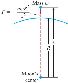
Escape velocity The gravitational attraction F exerted by an airless moon on a body of mass m at a distance s from the moon’s center is given by the equation $𝐹 = - 𝑚 𝑔 𝑅 2 𝑠 - 2$ , where $𝑔$ is the acceleration of gravity at the moon’s surface and R is the moon’s radius (see accompanying figure). The force F is negative because it acts in the direction of decreasing s.

教材插图

a. If the body is projected vertically upward from the moon’s surface with an initial velocity $𝑣 0$ at time $𝑡 = 0$ , use Newton’s second law, $𝐹 = 𝑚 𝑎,$ to show that the body’s velocity at position s is given by the equation

𝑣 2 = 2 𝑔 𝑅 2 𝑠 + 𝑣 20 - 2 𝑔 𝑅 .

Thus, the velocity remains positive as long as $𝑣 0 \geq \sqrt 2 𝑔 𝑅 .$ . The velocity $𝑣 0 = \sqrt 2 𝑔 𝑅$ is the moon’s escape velocity. A body projected upward with this velocity or a greater one will escape from the moon’s gravitational pull.

b. Show that if $𝑣 0 = \sqrt 2 𝑔 𝑅$ , then

𝑠 = 𝑅 (1 + 3 𝑣 0 2 𝑅 𝑡) 2 / 3 .

Coasting to a stop Table 16.6 shows the distance s (meters) coasted on inline skates in t s by Johnathon Krueger. Find a model for his position in the form of Equation (2) of Section 16.3. His initial velocity was $𝑣 0 = 0.86 m / s$ , his mass $𝑚 = 30.84 k g$ and his total coasting distance was 0.97 m.

TABLE 16.6 Johnathon Krueger skating data

t(s)	s(m)	t(s)	s(m)	t(s)	s(m)
0	0	0.93	0.61	1.86	0.93
0.13	0.08	1.06	0.68	2.00	0.94
0.27	0.19	1.20	0.74	2.13	0.95
0.40	0.28	1.33	0.79	2.26	0.96
0.53	0.36	1.46	0.83	2.39	0.96
0.67	0.45	1.60	0.87	2.53	0.97
0.80	0.53	1.73	0.90	2.66	0.97

Mixture Problems

In Exercises 43 and 44, let S represent the kilograms of salt in a tank at time t minutes. Set up a differential equation representing the given information and the rate at which S changes. Then solve for S and answer the particular questions.

A mixture containing $14$ kg of salt per liter flows into a tank at the rate of 24 $L / m i n,$ and the well-stirred mixture flows out of the tank at the rate of 16 L/min. The tank initially holds 600 liters of solution containing 6 kilograms of salt.

a. How many liters of solution are in the tank after 1 minute? after 10 minutes? after 1 hour?

b. How many kilograms of salt are in the tank after 1 minute? after 10 minutes? after 1 hour?

Pure water flows into a tank at the rate of $16 L / m i n$ , and the wellstirred mixture flows out of the tank at the rate of 20 L/min. The tank initially holds 800 liters of solution containing 25 kilograms of salt.

a. How many liters of solution are in the tank after 1 minute? after 10 minutes? after 200 minutes?

b. How many kilograms of salt are in the tank after 1 minute? after 30 minutes?

c. When will the tank have exactly 5 kilograms of salt, and how many liters of solution will be in the tank?

CHAPTER 16 Additional and Advanced Exercises

Theory and Applications

Transport through a cell membrane Under some conditions, the result of the movement of a dissolved substance across a cell’s membrane is described by the equation

𝑑 𝑦 𝑑 𝑡 = 𝑘 𝐴 𝑉 (𝑐 - 𝑦) .

In this equation, y is the concentration of the substance inside the cell, and $𝑑 𝑦 / 𝑑 𝑡$ is the rate at which y changes over time. The letters $𝑘, 𝐴, 𝑉,$ and c stand for constants, k being the permeability coefficient (a property of the membrane), A the surface area of the membrane, V the cell’s volume, and c the concentration of the substance outside the cell. The equation says that the rate at which the concentration within the cell changes is proportional to the difference between it and the outside concentration.

a. Solve the equation for $𝑦 (𝑡),$ , using $𝑦 0$ to denote $𝑦 (0)$

b. Find the steady-state concentration, lim $𝑦 (𝑡)$

Height of a rocket If an external force F acts upon a system whose mass varies with time, Newton’s law of motion is

𝑑 (𝑚 𝑣) 𝑑 𝑡 = 𝐹 + (𝑣 + 𝑢) 𝑑 𝑚 𝑑 𝑡 .

In this equation, m is the mass of the system at time $𝑡, 𝜐$ is its velocity, and $𝜐 + 𝑢$ is the velocity of the mass that is entering (or leaving) the system at the rate $𝑑 𝑚 / 𝑑 𝑡$ . Suppose that a rocket of initial mass $𝑚 0$ starts from rest, but is driven upward by firing some of its mass directly backward at the constant rate of $𝑑 𝑚 / 𝑑 𝑡 = - 𝑏$ units per second and at constant speed relative to the rocket $𝑢 = - 𝑐 .$ The only external force acting on the rocket is $𝐹 = - 𝑚 𝑔$ due to gravity. Under these assumptions, show that the height of the rocket above the ground at the end of t seconds (t small compared to $𝑚 0 / 𝑏)$ is

𝑦 = 𝑐 [𝑡 + 𝑚 0 - 𝑏 𝑡 𝑏 l n 𝑚 0 - 𝑏 𝑡 𝑚 0] - 12 𝑔 𝑡 2 .

a. Assume that $𝑃 (𝑥)$ and $𝑄 (𝑥)$ are continuous over the interval $[𝑎, 𝑏]$ . Use the Fundamental Theorem of Calculus, Part 1, to show that any function y satisfying the equation

𝑣 (𝑥) 𝑦 = \int 𝑣 (𝑥) 𝑄 (𝑥) 𝑑 𝑥 + 𝐶

for $𝑣 (𝑥) = 𝑒 \int 𝑃 (𝑥) 𝑑 𝑥$ is a solution to the first-order linear equation

𝑑 𝑦 𝑑 𝑥 + 𝑃 (𝑥) 𝑦 = 𝑄 (𝑥) .

b. If $\nabla' 𝐶 = 𝑦 0 𝑣 (𝑥 0) - \int 𝑥 𝑥 0 𝑣 (𝑡) 𝑄 (𝑡) 𝑑 𝑡$ , then show that any solution y in part (a) satisfies the initial condition $𝑦 (𝑥 0) = 𝑦 0$

(Continuation of Exercise 3.) Assume the hypotheses of Exercise 3, and assume that $𝑦 1 (𝑥)$ and $𝑦 2 (𝑥)$ are both solutions to the first-order linear equation satisfying the initial condition $𝑦 (𝑥 0) = 𝑦 0 .$

a. Verify that $𝑦 (𝑥) = 𝑦 1 (𝑥) - 𝑦 2 (𝑥)$ satisfies the initial value problem

𝑦' + 𝑃 (𝑥) 𝑦 = 0, 𝑦 (𝑥 0) = 0 .

b. For the integrating factor $𝑣 (𝑥) = 𝑒 \int 𝑃 (𝑥) 𝑑 𝑥$ , show that

𝑑 𝑑 𝑥 (𝑣 (𝑥) [𝑦 1 (𝑥) - 𝑦 2 (𝑥)]) = 0 .

Conclude that $𝑣 (𝑥) [𝑦 1 (𝑥) - 𝑦 2 (𝑥)] \equiv$ constant.

c. From part (a), we have $𝑦 1 (𝑥 0) - 𝑦 2 (𝑥 0) = 0$ . Since $𝑣 (𝑥) > 0$ for a $< 𝑥 < 𝑏 .$ , use part (b) to establish that $𝑦 1 (𝑥) - 𝑦 2 (𝑥) \equiv 0$ on the interval $(𝑎, 𝑏)$ . Thus $𝑦 1 (𝑥) = 𝑦 2 (𝑥)$ for all $𝑎 < 𝑥 < 𝑏 .$

Homogeneous Equations

A first-order diferential equation of the form

𝑑 𝑦 𝑑 𝑥 = 𝐹 (𝑦 𝑥)

is called homogeneous. It can be transformed into an equation whose variables are separable by defining the new variable $𝜐 = 𝑦 / 𝑥$ . Then $𝑦 = 𝑣 𝑥$ and

𝑑 𝑦 𝑑 𝑥 = 𝑣 + 𝑥 𝑑 𝑣 𝑑 𝑥 .

Substituting into the original diferential equation and collecting terms with like variables then give the separable equation

𝑑 𝑥 𝑥 + 𝑑 𝑣 𝑣 - 𝐹 (𝑣) = 0 .

After solving this separable equation, we obtain the solution of the original equation when we replace υ by $𝑦 / 𝑥$

Solve the homogeneous equations in Exercises 5–10. First put the equation in the form of a homogeneous equation.

$(𝑥 2 + 𝑦 2) 𝑑 𝑥 + 𝑥 𝑦 𝑑 𝑦 = 0$

𝑥 2 𝑑 𝑦 + (𝑦 2 - 𝑥 𝑦) 𝑑 𝑥 = 0

7 . (𝑥 𝑒 𝑦 / 𝑥 + 𝑦) 𝑑 𝑥 - 𝑥 𝑑 𝑦 = 0

(𝑥 + 𝑦) 𝑑 𝑦 + (𝑥 - 𝑦) 𝑑 𝑥 = 0

𝑦' = 𝑦 𝑥 + c o s 𝑦 - 𝑥 𝑥

$(𝑥 s i n 𝑦 𝑥 - 𝑦 c o s 𝑦 𝑥) 𝑑 𝑥 + 𝑥 c o s 𝑦 𝑥 𝑑 𝑦 = 0$

CHAPTER 16 Technology Application Projects

Mathematica/Maple Projects

Projects can be found within MyLab Math.

• Drug Dosages: Are They Effective? Are They Safe? Formulate and solve an initial value model for the absorption of a drug in the bloodstream.

• First-Order Differential Equations and Slope Fields Plot slope fields and solution curves for various initial conditions to selected first-order differential equations.

This page is intentionally left blank