Chapter 17: Second-Order Differential Equations

Denis Kalinichenko/Shutterstock
OVERVIEW In this chapter we extend our study of differential equations to those of second order, equations that involve second derivatives of a function. Second-order differential equations arise in many applications in the sciences and engineering. For instance, they can be applied to the study of vibrating springs and electric circuits. You will learn how to solve such differential equations by several methods in this chapter.
17.1 Second-Order Linear Equations
An equation of the form
which is linear in
We also assume that
Two fundamental results are important to solving Equation (2). The first of these says that if we know two solutions
THEOREM 1—The Superposition Principle
If
is also a solution to Equation (2).
Proof Substituting y into Equation (2), we have
Therefore,
Theorem 1 immediately establishes the following facts concerning solutions to the linear homogeneous equation.
-
A sum of two solutions
𝑦 1 + 𝑦 2 𝑐 1 = 𝑐 2 = 1 . ) -
A constant multiple
𝑘 𝑦 1 𝑦 1 𝑐 1 = 𝑘 a n d 𝑐 2 = 0 . ) -
The trivial solution
𝑦 ( 𝑥 ) ≡ 0 𝑐 1 = 𝑐 2 = 0 . )
The second fundamental result about solutions to the linear homogeneous equation concerns its general solution, or solution containing all solutions. This result says that there are two solutions
THEOREM 2 If P, Q, and R are continuous over the open interval I and
where
We now turn our attention to finding two linearly independent solutions to the special case of Equation (2) where
Constant-Coefficient Homogeneous Equations
Suppose we wish to solve the second-order homogeneous differential equation
where
Since the exponential function is never zero, we can divide this last equation through by
Equation (4) is called the auxiliary equation (or characteristic equation) of the differential equation
There are three cases to consider, which depend on the value of the discriminant
Case 1:
THEOREM 3 If
is the general solution to
EXAMPLE 1 Find the general solution of the differential equation
Solution Substitution of
which factors as
The roots are
Case 2:
THEOREM 4 If
The first term is zero because
EXAMPLE 2 Find the general solution to
Solution The auxiliary equation is
which factors into
Thus,
Case 3:
(The expressions involving the sine and cosine terms follow from Euler’s identity, as seen in the discussion of Taylor series.) However, the solutions
The functions
THEOREM 5 If
is the general solution to
EXAMPLE 3 Find the general solution to the differential equation
Solution The auxiliary equation is
The roots are the complex pair
Initial Value and Boundary Value Problems
To determine a unique solution to a first-order linear differential equation, it was sufficient to specify the value of the solution at a single point. Since the general solution to a secondorder equation contains two arbitrary constants, it is necessary to specify two conditions. One way of doing this is to specify the value of the solution function and the value of its derivative at a single point:
THEOREM 6 If P Q, , R, and G are continuous throughout an open interval I, then there exists one and only one function
on the interval I, and the initial conditions
at the specified point
It is important to realize that any real values can be assigned to
EXAMPLE 4 Find the particular solution to the initial value problem
Solution The auxiliary equation is
The repeated real root is
Then
From the initial conditions we have
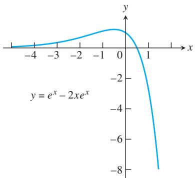
FIGURE 17.1 Particular solution curve for Example 4.
Thus,
The solution curve is shown in Figure 17.1.
Another approach to determine the values of the two arbitrary constants in the general solution to a second-order differential equation is to specify the values of the solution function at two different points in the interval I. That is, we solve the differential equation subject to the boundary values
where
EXAMPLE 5 Solve the boundary value problem
Solution The auxiliary equation is
The boundary conditions are satisfied if
It follows that
Exercises 17.1
In Exercises 1–30, find the general solution of the given equation.
-
𝑦 ′ ′ − 𝑦 ′ − 1 2 𝑦 = 0 -
3 𝑦 ′ ′ − 𝑦 ′ = 0 -
𝑦 ′ ′ + 3 𝑦 ′ − 4 𝑦 = 0 -
𝑦 ′ ′ − 9 𝑦 = 0 -
𝑦 ′ ′ − 4 𝑦 = 0 -
𝑦 ′ ′ − 6 4 𝑦 = 0 -
2 𝑦 ′ ′ − 𝑦 ′ − 3 𝑦 = 0 -
9 𝑦 ′ ′ − 𝑦 = 0 -
8 𝑦 ′ ′ − 1 0 𝑦 ′ − 3 𝑦 = 0 -
3 𝑦 ′ ′ − 2 0 𝑦 ′ + 1 2 𝑦 = 0 -
𝑦 ′ ′ + 9 𝑦 = 0 -
𝑦 ′ ′ + 4 𝑦 ′ + 5 𝑦 = 0 -
𝑦 ′ ′ + 2 5 𝑦 = 0 -
𝑦 ′ ′ + 𝑦 = 0 -
𝑦 ′ ′ − 2 𝑦 ′ + 5 𝑦 = 0 -
𝑦 ′ ′ + 1 6 𝑦 = 0 -
𝑦 ′ ′ + 2 𝑦 ′ + 4 𝑦 = 0 -
𝑦 ′ ′ − 2 𝑦 ′ + 3 𝑦 = 0 -
𝑦 ′ ′ + 4 𝑦 ′ + 9 𝑦 = 0 -
4 𝑦 ′ ′ − 4 𝑦 ′ + 1 3 𝑦 = 0 -
𝑦 ′ ′ = 0 -
𝑦 ′ ′ + 8 𝑦 ′ + 1 6 𝑦 = 0 -
𝑑 2 𝑦 𝑑 𝑥 2 + 4 𝑑 𝑦 𝑑 𝑥 + 4 𝑦 = 0 -
𝑑 2 𝑦 𝑑 𝑥 2 − 6 𝑑 𝑦 𝑑 𝑥 + 9 𝑦 = 0 -
𝑑 2 𝑦 𝑑 𝑥 2 + 6 𝑑 𝑦 𝑑 𝑥 + 9 𝑦 = 0 -
4 𝑑 2 𝑦 𝑑 𝑥 2 − 1 2 𝑑 𝑦 𝑑 𝑥 + 9 𝑦 = 0 -
4 𝑑 2 𝑦 𝑑 𝑥 2 + 4 𝑑 𝑦 𝑑 𝑥 + 𝑦 = 0 -
4 𝑑 2 𝑦 𝑑 𝑥 2 − 4 𝑑 𝑦 𝑑 𝑥 + 𝑦 = 0 -
9 𝑑 2 𝑦 𝑑 𝑥 2 + 6 𝑑 𝑦 𝑑 𝑥 + 𝑦 = 0 -
9 𝑑 2 𝑦 𝑑 𝑥 2 − 1 2 𝑑 𝑦 𝑑 𝑥 + 4 𝑦 = 0
In Exercises 31–40, find the unique solution of the second-order initial value problem.
-
𝑦 ′ ′ + 6 𝑦 ′ + 5 𝑦 = 0 , 𝑦 ( 0 ) = 0 , 𝑦 ′ ( 0 ) = 3 -
𝑦 ′ ′ + 1 6 𝑦 = 0 , 𝑦 ( 0 ) = 2 , 𝑦 ′ ( 0 ) = − 2 -
𝑦 ′ ′ + 1 2 𝑦 = 0 , 𝑦 ( 0 ) = 0 , 𝑦 ′ ( 0 ) = 1 -
1 2 𝑦 ′ ′ + 5 𝑦 ′ − 2 𝑦 = 0 , 𝑦 ( 0 ) = 1 , 𝑦 ′ ( 0 ) = − 1 -
y y ′′ + = 8 0, ( y y 0) = −1, (′ 0) = 2
-
y y′′ + 4 4′ + =y y0, (0) 0= , y′(0) 1=
-
𝑦 ′ ′ − 4 𝑦 ′ + 4 𝑦 = 0 , 𝑦 ( 0 ) = 1 , 𝑦 ′ ( 0 ) = 0 -
4 𝑦 ′ ′ − 4 𝑦 ′ + 𝑦 = 0 , 𝑦 ( 0 ) = 4 , 𝑦 ′ ( 0 ) = 4
In Exercises 41–55, find the general solution.
-
𝑦 ′ ′ − 2 𝑦 ′ − 3 𝑦 = 0 -
6 𝑦 ′ ′ − 𝑦 ′ − 𝑦 = 0 -
4 𝑦 ′ ′ + 4 𝑦 ′ + 𝑦 = 0 -
9 𝑦 ′ ′ + 1 2 𝑦 ′ + 4 𝑦 = 0 -
4 𝑦 ′ ′ + 2 0 𝑦 = 0 -
𝑦 ′ ′ + 2 𝑦 ′ + 2 𝑦 = 0 -
2 5 𝑦 ′ ′ + 1 0 𝑦 ′ + 𝑦 = 0 -
6 𝑦 ′ ′ + 1 3 𝑦 ′ − 5 𝑦 = 0 -
4 𝑦 ′ ′ + 4 𝑦 ′ + 5 𝑦 = 0
6 𝑦 ′ ′ − 5 𝑦 ′ − 4 𝑦 = 0
In Exercises 56–60, solve the initial value problem.
-
𝑦 ′ ′ − 2 𝑦 ′ + 2 𝑦 = 0 , 𝑦 ( 0 ) = 0 , 𝑦 ′ ( 0 ) = 2 -
𝑦 ′ ′ + 2 𝑦 ′ + 𝑦 = 0 , 𝑦 ( 0 ) = 1 , 𝑦 ′ ( 0 ) = 1 -
4 𝑦 ′ ′ − 4 𝑦 ′ + 𝑦 = 0 , 𝑦 ( 0 ) = − 1 , 𝑦 ′ ( 0 ) = 2 -
3 𝑦 ′ ′ + 𝑦 ′ − 1 4 𝑦 = 0 , 𝑦 ( 0 ) = 2 , 𝑦 ′ ( 0 ) = − 1 -
4 𝑦 ′ ′ + 4 𝑦 ′ + 5 𝑦 = 0 , 𝑦 ( 𝜋 ) = 1 , 𝑦 ′ ( 𝜋 ) = 0 -
Prove that the two solution functions in Theorem 3 are linearly independent.
-
Prove that the two solution functions in Theorem 4 are linearly independent.
-
Prove that the two solution functions in Theorem 5 are linearly independent.
-
Prove that if
𝑦 1 𝑦 2 𝑦 3 = 𝑦 1 + 𝑦 2 𝑦 4 = 𝑦 1 − 𝑦 2 -
a. Show that there is no solution to the boundary value problem
b. Show that there are infinitely many solutions to the boundary value problem
approach zero as
17.2 Nonhomogeneous Linear Equations
In this section we study two methods for solving second-order linear nonhomogeneous differential equations with constant coefficients. These are the methods of undetermined coefficients and variation of parameters. We begin by considering the form of the general solution.
Form of the General Solution
Suppose we wish to solve the nonhomogeneous equation
where
(We learned how to find
also solves the nonhomogeneous equation (1) because
Moreover, if
Thus,
THEOREM 7 The general solution
where the complementary solution
The Method of Undetermined Coefficients
This method for finding a particular solution
For instance,
EXAMPLE 1 Solve the nonhomogeneous equation
Solution The auxiliary equation for the complementary equation
It has the roots
Now
We need to determine the unknown coefficients A, B, and C. When we substitute the polynomial
or, collecting terms with like powers of
This last equation holds for all values of x if its two sides are identical polynomials of degree 2. Thus, we equate corresponding powers of x to get
These equations imply in turn that
By Theorem 7, the general solution to the nonhomogeneous equation is
EXAMPLE 2 Find a particular solution of
Solution If we try to find a particular solution of the form
and substitute the derivatives of
for all values of x. Since this requires A to equal both −2 and 0 at the same time, we conclude that the nonhomogeneous differential equation has no solution of the form A x sin .
It turns out that the required form is the sum
The result of substituting the derivatives of this new trial solution into the differential equation is
or
This last equation must be an identity. Equating the coefficients for like terms on each side then gives
Simultaneous solution of these two equations gives A = −1 and B = 1. Our particular solution is
EXAMPLE 3 Find a particular solution of
Solution If we substitute
and its derivatives into the differential equation, we find that
or
However, the exponential function is never zero. The trouble can be traced to the fact that
The auxiliary equation is
which has
The appropriate way to modify the trial solution in this case is to multiply
The result of substituting the derivatives of this new candidate into the differential equation is
or
Thus,
EXAMPLE 4 Find a particular solution of
Solution The auxiliary equation for the complementary equation
has
and its derivatives into the given differential equation, we get
or
Thus,
When we wish to find a particular solution of Equation (1) and the function
EXAMPLE 5 Find the general solution to
Solution We first check the auxiliary equation
Its roots are
We now seek a particular solution
Since any function of the form
including
or
This equation will hold if
or
The general solution to the differential equation is
You may find the following table helpful in solving the problems at the end of this section.
TABLE 17.1 The method of undetermined coefficients for selected equations of the form
| If | And if... | Then include this expression in the trial function for |
| r is not a root of the auxiliary equation | ||
| r is a single root of the auxiliary equation | ||
| r is a double root of the auxiliary equation | ||
| sin kx, cos kx | ki is not a root of the auxiliary equation | B cos kx + C sin kx |
| 0 is not a root of the auxiliary equation | ||
| 0 is a single root of the auxiliary equation | ||
| 0 is a double root of the auxiliary equation |
The Method of Variation of Parameters
This is a general method for finding a particular solution of the nonhomogeneous equation (1) once the general solution of the associated homogeneous equation is known. The method consists of replacing the constants
Then we have
If we substitute these expressions into the left-hand side of equation (1), we obtain
The first two parenthetical terms are zero since
Equations (4) and (5) can be solved together as a pair
for the unknown functions
Variation of Parameters Procedure
To use the method of variation of parameters to find a particular solution to the nonhomogeneous equation
we can work directly with Equations (4) and (5). It is not necessary to rederive them. The steps are as follows.
- Solve the associated homogeneous equation
to find the functions
- Solve the equations
simultaneously for the derivative functions
-
Integrate
𝑣 1 ′ 𝑣 2 ′ 𝑣 1 = 𝑣 1 ( 𝑥 ) 𝑣 2 = 𝑣 2 ( 𝑥 ) -
Write down the particular solution to the nonhomogeneous equation (1) as
EXAMPLE 6 Find the general solution to the equation
Solution The solution of the homogeneous equation
is given by
Since
Solving this system gives
Likewise,
After integrating
and
Note that we have omitted the constants of integration in determining
Substituting
The general solution is
EXAMPLE 7 Solve the nonhomogeneous equation
Solution The auxiliary equation is
giving the complementary solution
The conditions to be satisfied in Equations (4) and (5) are
Solving the above system for
Likewise,
Integrating to obtain the parameter functions, we have
and
Therefore,
The general solution to the differential equation is
where the term
Exercises 17.2
Solve the equations in Exercises 1–16 by the method of undetermined coefficients.
-
𝑦 ′ ′ − 3 𝑦 ′ − 1 0 𝑦 = − 3 -
𝑦 ′ ′ − 3 𝑦 ′ − 1 0 𝑦 = 2 𝑥 − 3 -
y y ′′ − ′ = sin x
-
𝑦 ′ ′ + 2 𝑦 ′ + 𝑦 = 𝑥 2 -
𝑦 ′ ′ + 𝑦 = c o s 3 𝑥 -
𝑦 ′ ′ + 𝑦 = 𝑒 2 𝑥 -
7 ′ ′ − 𝑦 ′ − 2 𝑦 = 2 0 c o s 𝑥 8 . 𝑦 ′ ′ + 𝑦 = 2 𝑥 + 3 𝑒 𝑥 -
𝑦 ′ ′ − 𝑦 = 𝑒 𝑥 + 𝑥 2 1 0 . 𝑦 ′ ′ + 2 𝑦 ′ + 𝑦 = 6 s i n 2 𝑥 -
𝑦 ′ ′ − 𝑦 ′ − 6 𝑦 = 𝑒 − 𝑥 − 7 c o s 𝑥 -
𝑦 ′ ′ + 3 𝑦 ′ + 2 𝑦 = 𝑒 − 𝑥 + 𝑒 − 2 𝑥 − 𝑥 -
𝑑 2 𝑦 𝑑 𝑥 2 + 5 𝑑 𝑦 𝑑 𝑥 = 1 5 𝑥 2 -
𝑑 2 𝑦 𝑑 𝑥 2 − 𝑑 𝑦 𝑑 𝑥 = − 8 𝑥 + 3 -
𝑑 2 𝑦 𝑑 𝑥 2 − 3 𝑑 𝑦 𝑑 𝑥 = 𝑒 3 𝑥 − 1 2 𝑥 -
𝑑 2 𝑦 𝑑 𝑥 2 + 7 𝑑 𝑦 𝑑 𝑥 = 4 2 𝑥 2 + 5 𝑥 + 1
Solve the equations in Exercises 17–28 by variation of parameters.
-
𝑦 ′ ′ + 𝑦 ′ = 𝑥 -
𝑦 ′ ′ + 𝑦 = t a n 𝑥 , − 𝜋 2 < 𝑥 < 𝜋 2 -
𝑦 ′ ′ + 𝑦 = s i n 𝑥 -
𝑦 ′ ′ + 2 𝑦 ′ + 𝑦 = 𝑒 𝑥 -
𝑦 ′ ′ + 2 𝑦 ′ + 𝑦 = 𝑒 − 𝑥 -
𝑦 ′ ′ − 𝑦 = 𝑥 -
𝑦 ′ ′ − 𝑦 = 𝑒 𝑥 -
𝑦 ′ ′ − 𝑦 = s i n 𝑥 -
𝑦 ′ ′ + 4 𝑦 ′ + 5 𝑦 = 1 0 -
𝑦 ′ ′ − 𝑦 ′ = 2 𝑥 -
𝑑 2 𝑦 𝑑 𝑥 2 + 𝑦 = s e c 𝑥 , − 𝜋 2 < 𝑥 < 𝜋 2 -
𝑑 2 𝑦 𝑑 𝑥 2 − 𝑑 𝑦 𝑑 𝑥 = 𝑒 𝑥 c o s 𝑥 , 𝑥 > 0
In each of Exercises 29–32, the given differential equation has a particular solution
-
𝑦 ′ ′ − 5 𝑦 ′ = 𝑥 𝑒 5 𝑥 , 𝑦 p = 𝐴 𝑥 2 𝑒 5 𝑥 + 𝐵 𝑥 𝑒 5 𝑥 -
𝑦 ′ ′ − 𝑦 ′ = c o s 𝑥 + s i n 𝑥 , 𝑦 p = 𝐴 c o s 𝑥 + 𝐵 s i n 𝑥 -
𝑦 ′ ′ + 𝑦 = 2 c o s 𝑥 + s i n 𝑥 , 𝑦 p = 𝐴 𝑥 c o s 𝑥 + -
𝑦 ′ ′ + 𝑦 ′ − 2 𝑦 = 𝑥 𝑒 𝑥 , 𝑦 p = 𝐴 𝑥 2 𝑒 𝑥 + 𝐵 𝑥 𝑒 𝑥
In Exercises 33–36, solve the given differential equations (a) by variation of parameters and (b) by the method of undetermined coefficients.
-
𝑑 2 𝑦 𝑑 𝑥 2 − 𝑑 𝑦 𝑑 𝑥 = 𝑒 𝑥 + 𝑒 − 𝑥 3 4 . 𝑑 2 𝑦 𝑑 𝑥 2 − 4 𝑑 𝑦 𝑑 𝑥 + 4 𝑦 = 2 𝑒 2 𝑥 -
𝑑 2 𝑦 𝑑 𝑥 2 − 4 𝑑 𝑦 𝑑 𝑥 − 5 𝑦 = 𝑒 𝑥 + 4 3 6 . 𝑑 2 𝑦 𝑑 𝑥 2 − 9 𝑑 𝑦 𝑑 𝑥 = 9 𝑒 9 𝑥
Solve the differential equations in Exercises 37–46. Some of the equations can be solved by the method of undetermined coefficients, but others cannot.
-
𝑦 ′ ′ + 𝑦 = c o t 𝑥 , 0 < 𝑥 < 𝜋 -
𝑦 ′ ′ + 𝑦 = c s c 𝑥 , 0 < 𝑥 < 𝜋 -
𝑦 ′ ′ − 8 𝑦 ′ = 𝑒 8 𝑥 -
𝑦 ′ ′ + 4 𝑦 = s i n 𝑥 -
𝑦 ′ ′ − 𝑦 ′ = 𝑥 3 4 2 . 𝑦 ′ ′ + 4 𝑦 ′ + 5 𝑦 = 𝑥 + 2
17.3 Applications
Vibrations
𝑦 ′ ′ − 3 𝑦 ′ + 2 𝑦 = 𝑒 𝑥 − 𝑒 2 𝑥
The method of undetermined coefficients can sometimes be used to solve first-order ordinary differential equations. Use the method to solve the equations in Exercises 47–50.
Solve the differential equations in Exercises 51 and 52 subject to the given initial conditions.
In Exercises 53–58, verify that the given function is a particular solution to the specified nonhomogeneous equation. Find the general solution, and evaluate its arbitrary constants to find the unique solution satisfying the equation and the given initial conditions.
In Exercises 59 and 60, two linearly independent solutions
In this section we apply second-order differential equations to the study of vibrating springs and electric circuits.
A spring has its upper end fastened to a rigid support, as shown in Figure 17.2. An object of mass m is suspended from the spring and stretches it a length s when the spring comes to rest in an equilibrium position. According to Hooke’s Law (Section 6.5), the tension force in the spring is
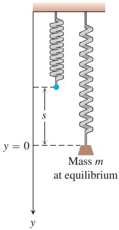
FIGURE 17.2 Mass m stretches a spring by length s to the equilibrium position at
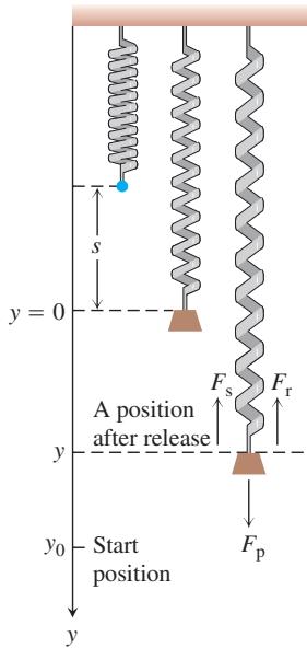
(weight)
Suppose that the object is pulled down an additional amount
Let
The frictional force tends to slow the motion of the object. The resultant of these forces is
By Equation (1),
subject to the initial conditions
You might expect that the motion predicted by Equation (2) will be oscillatory about the equilibrium position
Simple Harmonic Motion
Suppose first that there is no frictional force. Then
The auxiliary equation is
which has the imaginary roots
To fit the initial conditions, we compute
and then substitute the conditions. This yields
(4)
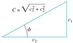
FIGURE 17.4
describes the motion of the object. Equation (4) represents simple harmonic motion of amplitude
The general solution given by Equation (3) can be combined into a single term by using the trigonometric identity
To apply the identity, we take (see Figure 17.4)
where
Then the general solution in Equation (3) can be written in the alternative form
Here C and
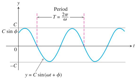
FIGURE 17.5 Simple harmonic motion of amplitude C and period T with initial phase angle φ (Equation 5).
Damped Motion
Assume now that there is friction in the spring system, so
The auxiliary equation is
with roots
Case 1:
This situation of motion is called critical damping and is not oscillatory. Figure 17.6a shows an example of this kind of damped motion.
Case 2:
Here again the motion is not oscillatory and both
Case 3:
This situation, called underdamping, represents damped oscillatory motion. It is analogous to simple harmonic motion of period
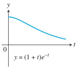
(a) Critical damping
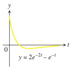
(b) Overdamping
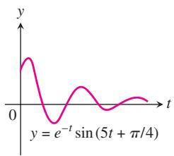
(c) Underdamping
FIGURE 17.6 Three examples of damped vibratory motion for a spring system with friction, so
An external force
Such equations are studied in the theory of Differential Equations.
Electric Circuits
The basic quantity in electricity is the charge q (analogous to the idea of mass). In an electric field we use the flow of charge, or current
Consider the electric circuit shown in Figure 17.7. It consists of four components: voltage source, resistor, inductor, and capacitor. Think of electrical flow as being like a fluid flow, where the voltage source is the pump and the resistor, inductor, and capacitor tend to block the flow. A battery or generator is an example of a source, producing a voltage that causes the current to flow through the circuit when the switch is closed. An electric light bulb or appliance would provide resistance. The inductance is due to a magnetic field that opposes any change in the current as it flows through a coil. The capacitance is normally created by two metal plates that alternate charges and thus reverse the current flow. The following symbols specify the quantities relevant to the circuit.
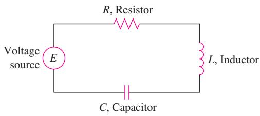
FIGURE 17.7 An electric circuit.
q: charge at a cross section of a conductor, measured in coulombs (abbreviated c)
I: current or rate of change of charge dq dt (flow of electrons) at a cross section of a conductor, measured in amperes (abbreviated A)
E: electric (potential) source, measured in volts (abbreviated V)
V: difference in potential between two points along the conductor, measured in volts (V)
Ohm observed that the current I flowing through a resistor, caused by a potential difference across it, is (approximately) proportional to the potential difference (voltage drop). He named his constant of proportionality 1 R and called R the resistance. So Ohm’s law is
Similarly, it is known from physics that the voltage drops across an inductor and a capacitor are, respectively,
where L is the inductance and C is the capacitance (with q the charge on the capacitor).
The German physicist Gustav R. Kirchhoff (1824–1887) formulated the law that the sum of the voltage drops in a closed circuit is equal to the supplied voltage E ( )t . Symbolically, this says that
Since
The second-order differential equation (8), which models an electric circuit, has exactly the same form as Equation (7) modeling vibratory motion. Both models can be solved using the methods developed in Section 17.2.
Summary
The following chart summarizes our analogies between the physics of motion of an object in a spring system and the flow of charged particles in an electric circuit.
| Linear Second-Order Constant-Coefficient Models | ||
| Mechanical System | Electrical System | |
| y | displacement | q charge |
| velocity | ||
| acceleration | ||
| m | mass | L inductance |
| δ | damping constant | R resistance |
| k | spring constant | |
| forcing function | ||
EXERCISES 17.3
-
A 70-N weight is attached to the lower end of a coil spring suspended from the ceiling and having a spring constant of
1 5 : N / m . 𝐀 𝔱 : = 0 -
A 36-N weight stretches a spring 1.2 m. The spring–mass system resides in a medium offering a resistance to the motion that is numerically equal to 20 times the instantaneous velocity. If the weight is released at a position 0.6 m above its equilibrium position with a downward velocity of 0.9
m / s , -
A 90-N weight is hung on a 0.4-m spring and stretches it 0.15 m. The weight is pulled down 0.1 m and 30 N are added to the weight. If the weight is now released with a downward velocity of
𝑣 0 m / s -
A 49-N weight is suspended by a spring that is stretched 0.05 m by the weight. Assume a resistance whose magnitude is
3 0 0 / √ 𝑔 -
An (open) electric circuit consists of an inductor, a resistor, and a capacitor. There is an initial charge of 2 coulombs on the capacitor. At the instant the circuit is closed, a current of 3 amperes is present and a voltage of
𝐸 ( 𝑡 ) = 2 0 -
An inductor of 2 henrys is connected in series with a resistor of 12 ohms, a capacitor of 1 16 farad, and a 300-volt battery.
Initially, the charge on the capacitor is zero and the current is zero. Formulate an initial value problem modeling this electric circuit.
-
A 49-N weight is attached to the lower end of a coil spring suspended from the ceiling and having a spring constant of
1 0 : N / m . -
A 29.4-N weight stretches a spring 1.225 m. The spring–mass system resides in a medium offering a resistance to the motion equal to 18 times the instantaneous velocity. If the weight is released at a position 0.6 m above its equilibrium position with a downward velocity of 0.9 m/s, find its position relative to the equilibrium position 2 s later.
-
A 98-N weight is hung on a 0.6 m spring stretching it 0.2 m. The weight is pulled down 0.15 m and 49 N are added to the weight. If the weight is now released with a downward velocity of
𝑣 0 𝑣 0 𝑡 ≥ 0 -
A mass of 15 kg is attached to a spring whose constant is 375/4 N/m. Initially the mass is released 1 m above the equilibrium position with a downward velocity of 3 m/s, and the subsequent motion takes place in a medium that offers a damping force numerically equal to 45 times the instantaneous velocity. An external force
𝑓 ( 𝑡 ) 𝑓 ( 𝑡 ) ≡ 0 -
A 50-N weight is suspended by a spring that is stretched 0.05 m by the weight. Assume a resistance whose magnitude is 100 N times the instantaneous velocity in meters per second. If the weight is pulled down 0.1 m below its equilibrium position and released, find the time required to reach the equilibrium position for the first time.
-
A weight stretches a spring 0.2 m. It is set in motion at a point 0.05 m below its equilibrium position with a downward velocity of 0.05 m/s. a. When does the weight return to its equilibrium position? b. When does it reach its highest point? c. Show that the maximum velocity is
0 . 0 5 √ 1 0 𝑔 m / s -
A weight of 50 N stretches a spring 0.25 m. The weight is drawn down 0.05 m below its equilibrium position and given an initial velocity of 0.1 m/s. An identical spring has a different weight attached to it. This second weight is drawn down from its equilibrium position a distance equal to the amplitude of the first motion and then given an initial velocity of 0.6 m/s. If the amplitude of the second motion is twice that of the first, what weight is attached to the second spring?
-
A weight stretches one spring 0.05 m and a second weight stretches another spring 0.15 m. If both weights are simultaneously pulled down 0.02 m below their respective equilibrium positions and then released, find the first time after t = 0 when their velocities are equal.
-
A weight of 80 N stretches a spring 1 m. The weight is pulled down 1.5 m below the equilibrium position and then released. What initial velocity
𝑣 0 -
A mass weighing 40 N stretches a spring 0.1 m. The spring– mass system resides in a medium with a damping constant of 32 N-s/m. If the mass is released from its equilibrium position with a velocity of 0.1 m/s in the downward direction, find the time required for the mass to return to its equilibrium position for the first time.
-
A weight suspended from a spring executes damped vibrations with a period of 2 s. If the damping factor decreases by 90% in 10 s, find the acceleration of the weight when it is 0.1 m below its equilibrium position and is moving upward with a speed of 0.8 m/s.
-
A 50-N weight stretches a spring 0.6 m. If the weight is pulled down 0.15 m below its equilibrium position and released, find the highest point reached by the weight. Assume the spring–mass system resides in a medium offering a resistance of 30 N times the instantaneous velocity in meters per second.
-
An LRC circuit is set up with an inductance of 1 5 henry, a resistance of 1 ohm, and a capacitance of 5 6 farad. Assuming the initial charge is 2 coulombs and the initial current is 4 amperes, find the solution function describing the charge on the capacitor at any time. What is the charge on the capacitor after a long period of time?
-
An (open) electric circuit consists of an inductor, a resistor, and a capacitor. There is an initial charge of 2 coulombs on the capacitor. At the instant the circuit is closed, a current of 3 amperes is present but no external voltage is being applied. In this circuit the voltage drops at three points are numerically related as follows: across the capacitor, 10 times the charge; across the resistor, 4 times the instantaneous change in the charge; and across the inductor, 2 times the instantaneous change in the current. Find the charge on the capacitor as a function of time.
-
A 78.4-N weight stretches a spring 1.225 m. This spring–mass system is in a medium with a damping constant of
7 2 N − s / m 𝑓 ( 𝑡 ) = 2 5 . 6 + 6 . 4 𝑒 − 2 𝑡 -
A 10-kg mass is attached to a spring having a spring constant of 140 N m. The mass is started in motion from the equilibrium position with an initial velocity of 1 m s in the upward direction and with an applied external force given by f( )t t= 5 sin (in newtons). The mass is in a viscous medium with a coefficient of resistance equal to 90 N-s m. Formulate an initial value problem that models the given system; solve the model and interpret the results.
-
A 2-kg mass is attached to the lower end of a coil spring suspended from the ceiling. The mass comes to rest in its equilibrium position thereby stretching the spring 1.96 m. The mass is in a viscous medium that offers a resistance in newtons numerically equal to 4 times the instantaneous velocity measured in meters per second. The mass is then pulled down 2 m below its equilibrium position and released with a downward velocity of 3 m s. At this same instant an external force given by f( )t = 20 cos t (in newtons) is applied to the system. At the end of π s determine if the mass is above or below its equilibrium position and by how much.
-
A 39.2-N weight stretches a spring 1.225 m. The spring–mass system resides in a medium offering a resistance to the motion equal to 24 times the instantaneous velocity, and an external force given by
𝑓 ( 𝑡 ) = 2 8 . 8 + 1 9 . 2 𝑒 − 𝑡 -
Suppose L = 10 henrys, R = 10 ohms, C = 1 500 farads, E = 100 volts, q(0) 1= 0 coulombs, and
𝑞 ′ ( 0 ) = 𝑖 ( 0 ) = 0 . -
A series circuit consisting of an inductor, a resistor, and a capacitor is open. There is an initial charge of 2 coulombs on the capacitor, and 3 amperes of current is present in the circuit at the instant the circuit is closed. A voltage given by E ( )t = 20 cos t is applied. In this circuit the voltage drops are numerically equal to the following: across the resistor, to 4 times the instantaneous change in the charge; across the capacitor, to 10 times the charge; and across the inductor, to 2 times the instantaneous change in the current. Find the charge on the capacitor as a function of time. Determine the charge on the capacitor and the current at time t = 10.
17.4 Euler Equations
In Section 17.1 we introduced the second-order linear homogeneous differential equation
and showed how to solve this equation when the coefficients
where
The General Solution of Euler Equations
Consider the Euler equation
To solve Equation (1), we first make the change of variables
We next use the chain rule to find the derivatives
and
Substituting these two derivatives into the left-hand side of Equation (1), we find
Therefore, the substitutions give us the second-order linear differential equation with constant coefficients
We can solve Equation (2) using the method of Section 17.1. That is, we find the roots of the associated auxiliary equation
to find the general solution for
EXAMPLE 1 Find the general solution of the equation
Solution This is an Euler equation with
with roots
Substituting z = ln x gives the general solution for y x( ):
EXAMPLE 2 Solve the Euler equation
Solution Since
The auxiliary equation has the double root
Substituting z = ln x into this expression gives the general solution
EXAMPLE 3 Find the particular solution to
Solution Here
The roots are
Substituting z = ln x into this expression gives
From the initial condition
To fit the second initial condition, we need the derivative
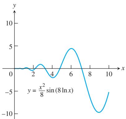
FIGURE 17.8 Graph of the solution to Example 3.
Since
Since
A graph of the solution is shown in Figure 17.8.
Exercises 17.4
In Exercises 1–24, find the general solution to the given Euler equation.
Assume
-
𝑥 2 𝑦 ′ ′ + 2 𝑥 𝑦 ′ − 2 𝑦 = 0 -
𝑥 2 𝑦 ′ ′ + 𝑥 𝑦 ′ − 4 𝑦 = 0 -
𝑥 2 𝑦 ′ ′ − 6 𝑦 = 0 -
𝑥 2 𝑦 ′ ′ + 𝑥 𝑦 ′ − 𝑦 = 0 -
𝑥 2 𝑦 ′ ′ − 5 𝑥 𝑦 ′ + 8 𝑦 = 0 -
2 7 x y′′ + xy′ + = 2 0 y 2
-
3 𝑥 2 𝑦 ′ ′ + 4 𝑥 𝑦 ′ = 0 -
𝑥 2 𝑦 ′ ′ + 6 𝑥 𝑦 ′ + 4 𝑦 = 0 -
𝑥 2 𝑦 ′ ′ − 𝑥 𝑦 ′ + 𝑦 = 0 -
𝑥 2 𝑦 ′ ′ − 𝑥 𝑦 ′ + 2 𝑦 = 0 -
𝑥 2 𝑦 ′ ′ − 𝑥 𝑦 ′ + 5 𝑦 = 0 -
𝑥 2 𝑦 ′ ′ + 7 𝑥 𝑦 ′ + 1 3 𝑦 = 0 -
𝑥 2 𝑦 ′ ′ + 3 𝑥 𝑦 ′ + 1 0 𝑦 = 0 -
𝑥 2 𝑦 ′ ′ − 5 𝑥 𝑦 ′ + 1 0 𝑦 = 0 -
4 𝑥 2 𝑦 ′ ′ + 8 𝑥 𝑦 ′ + 5 𝑦 = 0 -
4 𝑥 2 𝑦 ′ ′ − 4 𝑥 𝑦 ′ + 5 𝑦 = 0 -
𝑥 2 𝑦 ′ ′ + 3 𝑥 𝑦 ′ + 𝑦 = 0 -
𝑥 2 𝑦 ′ ′ − 3 𝑥 𝑦 ′ + 9 𝑦 = 0 -
𝑥 2 𝑦 ′ ′ + 𝑥 𝑦 ′ = 0 -
4 𝑥 2 𝑦 ′ ′ + 𝑦 = 0 -
9 𝑥 2 𝑦 ′ ′ + 1 5 𝑥 𝑦 ′ + 𝑦 = 0 -
1 6 𝑥 2 𝑦 ′ ′ − 8 𝑥 𝑦 ′ + 9 𝑦 = 0 -
1 6 𝑥 2 𝑦 ′ ′ + 5 6 𝑥 𝑦 ′ + 2 5 𝑦 = 0 -
4 𝑥 2 𝑦 ′ ′ − 1 6 𝑥 𝑦 ′ + 2 5 𝑦 = 0
In Exercises 25–30, solve the given initial value problem.
-
𝑥 2 𝑦 ′ ′ + 3 𝑥 𝑦 ′ − 3 𝑦 = 0 , 𝑦 ( 1 ) = 1 , 𝑦 ′ ( 1 ) = − 1 -
6 𝑥 2 𝑦 ′ ′ + 7 𝑥 𝑦 ′ − 2 𝑦 = 0 , 𝑦 ( 1 ) = 0 , 𝑦 ′ ( 1 ) = 1 -
𝑥 2 𝑦 ′ ′ − 𝑥 𝑦 ′ + 𝑦 = 0 , 𝑦 ( 1 ) = 1 , 𝑦 ′ ( 1 ) = 1 -
x y x ′′ + 7 9 y y ′ + = 0, y y (1) 1 = , (′ 1) = 0 2
-
𝑥 2 𝑦 ′ ′ − 𝑥 𝑦 ′ + 2 𝑦 = 0 , 𝑦 ( 1 ) = − 1 , 𝑦 ′ ( 1 ) = 1
17.5 Power-Series Solutions
In this section we extend our study of second-order linear homogeneous equations with variable coefficients. With the Euler equations in Section 17.4, the power of the variable x in the nonconstant coefficient had to match the order of the derivative with which it was paired:
Method of Solution
The power-series method for solving a second-order homogeneous differential equation consists of finding the coefficients of a power series
which solves the equation. To apply the method we substitute the series and its derivatives into the differential equation to determine the coefficients
In our first example we demonstrate the method in the setting of a simple equation whose general solution we already know. This is to help you become more comfortable with solutions expressed in series form.
EXAMPLE 1 Solve the equation
Solution We assume the series solution takes the form of
and calculate the derivatives
Substitution of these forms into the second-order equation gives us
Next, we equate the coefficients of each power of x to zero as summarized in the following table.
| Power of x | Coefficient equation | ||
| or | |||
| or | |||
| or | |||
| or | |||
| or | |||
| ⋮ | ⋮ | ⋮ | |
| or | |||
From the table we notice that the coefficients with even indices
Even indices: Here
or
From this recursive relation we find
Odd indices: Here
or
Thus,
Writing the power series by grouping its even and odd powers together and substituting for the coefficients yields
From our study of Taylor series, we see that the first series on the right-hand side of the last equation represents the cosine function, and the second series represents the sine. Thus, the general solution to
EXAMPLE 2 Find the general solution to
Solution We assume the series solution form
and calculate the derivatives
Substitution of these forms into the second-order equation yields
We equate the coefficients of each power of x to zero as summarized in the following table.
| Power of x | Coefficient equation | ||
| or | |||
| or | |||
| or | |||
| or | |||
| or | |||
| ⋮ | ⋮ | ⋮ | |
| or | |||
From the table notice that the coefficients with even indices are interrelated and the coefficients with odd indices are also interrelated.
Even indices: Here
From this recurrence relation we obtain
Odd indices: Here
From this recurrence relation we obtain
Writing the power series by grouping its even and odd powers and substituting for the coefficients yields
EXAMPLE 3 Find the general solution to
Solution Notice that the leading coefficient is zero when
and its derivatives gives us
Next, we equate the coefficients of each power of x to zero as summarized in the following table.
| Power of x | Coefficient equation | ||
| or | |||
| or | |||
| or | |||
| or | |||
| ⋮ | ⋮ | ⋮ | |
| or | |||
Again we notice that the coefficients with even indices are interrelated and those with odd indices are interrelated.
Even indices: Here
Odd indices: Here
The general solution is
EXAMPLE 4 Find the general solution to
Solution Assuming that
substitution into the differential equation gives us
We next determine the coefficients, listing them in the following table.
Power of x
Coefficient equation
From the recursive relation
we write out the first few terms of each series for the general solution:
Exercises 17.5
In Exercises 1–18, use power series to find the general solution of the differential equation.
-
𝑦 ′ ′ + 2 𝑦 ′ = 0 -
𝑦 ′ ′ + 2 𝑦 ′ + 𝑦 = 0 -
𝑦 ′ ′ + 4 𝑦 = 0 -
𝑦 ′ ′ − 3 𝑦 ′ + 2 𝑦 = 0 -
𝑥 2 𝑦 ′ ′ − 2 𝑥 𝑦 ′ + 2 𝑦 = 0 -
𝑦 ′ ′ − 𝑥 𝑦 ′ + 𝑦 = 0 -
( 1 + 𝑥 ) 𝑦 ′ ′ − 𝑦 = 0 -
( 1 − 𝑥 2 ) 𝑦 ′ ′ − 4 𝑥 𝑦 ′ + 6 𝑦 = 0 -
( 𝑥 2 − 1 ) 𝑦 ′ ′ + 2 𝑥 𝑦 ′ − 2 𝑦 = 0 -
𝑦 ′ ′ + 𝑦 ′ − 𝑥 2 𝑦 = 0 -
( 𝑥 2 − 1 ) 𝑦 ′ ′ − 6 𝑦 = 0 -
𝑥 𝑦 ′ ′ − ( 𝑥 + 2 ) 𝑦 ′ + 2 𝑦 = 0 -
( 𝑥 2 − 1 ) 𝑦 ′ ′ + 4 𝑥 𝑦 ′ + 2 𝑦 = 0 -
𝑦 ′ ′ − 2 𝑥 𝑦 ′ + 4 𝑦 = 0 -
𝑦 ′ ′ − 2 𝑥 𝑦 ′ + 3 𝑦 = 0 -
( 1 − 𝑥 2 ) 𝑦 ′ ′ − 𝑥 𝑦 ′ + 4 𝑦 = 0 -
𝑦 ′ ′ − 𝑥 𝑦 ′ + 3 𝑦 = 0 -
𝑥 2 𝑦 ′ ′ − 4 𝑥 𝑦 ′ + 6 𝑦 = 0
Chapter 17
SECTION 17.1, pp. 17-6–17-7
-
𝑦 = 𝑐 1 𝑒 − 3 𝑥 + 𝑐 2 𝑒 4 𝑥 𝑦 = 𝑐 1 𝑒 − 4 𝑥 + 𝑐 2 𝑒 𝑥 -
𝑦 = 𝑐 1 𝑒 − 2 𝑥 + 𝑐 2 𝑒 2 𝑥 𝑦 = 𝑐 1 𝑒 − 𝑥 + 𝑐 2 𝑒 3 𝑥 / 2 -
𝑦 = 𝑐 1 𝑒 − 𝑥 / 4 + 𝑐 2 𝑒 3 𝑥 / 2 𝟏 𝟏 . 𝑦 = 𝑐 1 c o s 3 𝑥 + 𝑐 2 s i n 3 𝑥 -
𝑦 = 𝑐 1 c o s 5 𝑥 + 𝑐 2 s i n 5 𝑥 1 5 . 𝑦 = 𝑒 𝑥 ( 𝑐 1 c o s 2 𝑥 + 𝑐 2 s i n 2 𝑥 ) -
𝑦 = 𝑒 − 𝑥 ( 𝑐 1 c o s √ 3 𝑥 + 𝑐 2 s i n √ 3 𝑥 ) -
𝑦 = 𝑒 − 2 𝑥 ( 𝑐 1 c o s √ 5 𝑥 + 𝑐 2 s i n √ 5 𝑥 ) -
𝑦 = 𝑐 1 + 𝑐 2 𝑥 2 3 . 𝑦 = 𝑐 1 𝑒 − 2 𝑥 + 𝑐 2 𝑥 𝑒 − 2 𝑥 -
𝑦 = 𝑐 1 𝑒 − 3 𝑥 + 𝑐 2 𝑥 𝑒 − 3 𝑥 𝑦 = 𝑐 1 𝑒 − 𝑥 / 2 + 𝑐 2 𝑥 𝑒 − 𝑥 / 2 -
𝑦 = 𝑐 1 𝑒 − 𝑥 / 3 + 𝑐 2 𝑥 𝑒 − 𝑥 / 3 𝑦 = − 3 4 𝑒 − 5 𝑥 + 3 4 𝑒 − 𝑥 -
𝑦 = 1 2 √ 3 s i n 2 √ 3 𝑥 -
𝑦 = − c o s 2 √ 2 𝑥 + 1 √ 2 s i n 2 √ 2 𝑥 -
𝑦 = ( 1 − 2 𝑥 ) 𝑒 2 𝑥 3 9 . 𝑦 = 2 ( 1 + 2 𝑥 ) 𝑒 − 3 𝑥 / 2 -
𝑦 = 𝑐 1 𝑒 − 𝑥 + 𝑐 2 𝑒 3 𝑥 𝑦 = 𝑐 1 𝑒 − 𝑥 / 2 + 𝑐 2 𝑥 𝑒 − 𝑥 / 2 -
𝑦 = 𝑐 1 c o s √ 5 𝑥 + 𝑐 2 s i n √ 5 𝑥 𝑦 = 𝑐 1 𝑒 − 𝑥 / 5 + 𝑐 2 𝑥 𝑒 − 𝑥 / 5 -
𝑦 = 𝑒 − 𝑥 / 2 ( 𝑐 1 c o s 𝑥 + 𝑐 2 s i n 𝑥 ) 𝑦 = 𝑐 1 𝑒 3 𝑥 / 4 + 𝑐 2 𝑥 𝑒 3 𝑥 / 4 -
𝑦 = 𝑐 1 𝑒 − 4 𝑥 / 3 + 𝑐 2 𝑥 𝑒 − 4 𝑥 / 3 𝑦 = 𝑐 1 𝑒 − 𝑥 / 2 + 𝑐 2 𝑒 4 𝑥 / 3 -
𝑦 = ( 1 + 2 𝑥 ) 𝑒 − 𝑥 𝑦 = 1 5 1 3 𝑒 − 7 𝑥 / 3 + 1 1 1 3 𝑒 2 𝑥
SECTION 17.2, pp. 17-14–17-15
𝑦 = 𝑐 1 𝑒 5 𝑥 + 𝑐 2 𝑒 − 2 𝑥 + 3 1 0
1 1 3. y c = + c e +x 1 2 −x2 cos x 2 sin
1 5. y c = + cos s x c in x − 1 2 x 8 cos 3
-
𝑦 = 𝑐 1 𝑒 2 𝑥 + 𝑐 2 𝑒 − 𝑥 − 6 c o s 𝑥 − 2 s i n 𝑥 -
y c = + e c e x − − − 2 + x x 2 12 xe x
-
y c = + c e− + + x 35x 1 2 5 3 x 2 − 6 x 25
-
𝑦 = 𝑐 1 + 𝑐 2 𝑒 3 𝑥 + 2 𝑥 2 + 4 3 𝑥 + 1 3 𝑥 𝑒 3 𝑥 -
𝑦 = 𝑐 1 + 𝑐 2 𝑒 − 𝑥 + 1 2 𝑥 2 − 𝑥 -
𝑦 = 𝑐 1 c o s 𝑥 + 𝑐 2 s i n 𝑥 − 1 2 𝑥 c o s 𝑥 -
𝑦 = ( 𝑐 1 + 𝑐 2 𝑥 ) 𝑒 − 𝑥 + 1 2 𝑥 2 𝑒 − 𝑥 -
𝑦 = 𝑐 1 𝑒 𝑥 + 𝑐 2 𝑒 − 𝑥 + 1 2 𝑥 𝑒 𝑥 -
𝑦 = 𝑒 − 2 𝑥 ( 𝑐 1 c o s 𝑥 + 𝑐 2 s i n 𝑥 ) + 2 -
𝑦 = 𝐴 c o s 𝑥 + -
𝑦 = 𝑐 1 + 𝑐 2 𝑒 5 𝑥 + 1 1 0 𝑥 2 𝑒 5 𝑥 − 1 2 5 𝑥 𝑒 5 𝑥 -
𝑦 = 𝑐 1 c o s 𝑥 + 𝑐 2 s i n 𝑥 − 1 2 𝑥 c o s 𝑥 + 𝑥 s i n 𝑥 -
𝑦 = 𝑐 1 + 𝑐 2 𝑒 𝑥 + 1 2 𝑒 − 𝑥 + 𝑥 𝑒 𝑥 -
𝑦 = 𝑐 1 𝑒 5 𝑥 + 𝑐 2 𝑒 − 𝑥 − 1 8 𝑒 𝑥 − 4 5 -
𝑦 = 𝑐 1 c o s 𝑥 + 𝑐 2 s i n 𝑥 − ( s i n 𝑥 ) [ l n ( c s c 𝑥 + c o t 𝑥 ) ] -
𝑦 = 𝑐 1 + 𝑐 2 𝑒 8 𝑥 + 1 8 𝑥 𝑒 8 𝑥 -
𝑦 = 𝑐 1 + 𝑐 2 𝑒 𝑥 − 𝑥 4 / 4 − 𝑥 3 − 3 𝑥 2 − 6 𝑥 -
𝑦 = 𝑐 1 + 𝑐 2 𝑒 − 2 𝑥 − 1 3 𝑒 𝑥 + 𝑥 3 / 6 − 𝑥 2 / 4 + 𝑥 / 4 -
𝑦 = 𝑐 1 c o s 𝑥 + 𝑐 2 s i n 𝑥 + ( 𝑥 − t a n 𝑥 ) c o s 𝑥 − s i n 𝑥 l n ( c o s 𝑥 ) = 𝑐 1 c o s 𝑥 + 𝑐 2 ′ s i n 𝑥 + 𝑥 c o s 𝑥 − ( s i n 𝑥 ) l n ( c o s 𝑥 ) -
𝑦 = 𝑐 𝑒 3 𝑥 − 1 2 𝑒 𝑥 -
𝑦 = 𝑐 𝑒 3 𝑥 + 5 𝑥 𝑒 3 𝑥 -
y x = + 2 cos sin 1 x x − + sin ln s( ) ec ta x x + n
-
𝑦 = − 𝑒 − 𝑥 + 1 + 1 2 𝑥 2 − 𝑥 -
𝑦 = 2 ( 𝑒 𝑥 − 𝑒 − 𝑥 ) c o s 𝑥 − 3 𝑒 − 𝑥 s i n 𝑥 -
𝑦 = ( 1 − 𝑥 + 𝑥 2 ) 𝑒 𝑥 -
𝑦 𝚙 = 1 4 𝑥 2
SeCtion 17.3, pp. 17-20–17-21
. 12 y″ + y′ + y = 0, y(0) = 0.6, y′(0) = 0.6 1 1
-
1 2 0 𝑦 ′ ′ + 6 0 0 𝑦 = 0 , -
2 𝑞 ′ ′ + 4 𝑞 ′ + 1 0 𝑞 = 2 0 c o s 𝑡 , 𝑞 ′ ( 0 ) = 3 -
0 . 0 2 5 9 m ( a b o v e e q u i l i b r i u m ) -
𝑦 ( 𝑡 ) = 0 . 0 5 c o s ( 5 . 7 1 5 𝑡 ) + 𝜐 0 5 . 7 1 5 s i n ( 5 . 7 1 5 𝑡 ) -
1.806 s 13. 45 N 15.
8 . 1 3 m / s -
0 . 6 2 3 8 m / s 2 ( a c c e l e r a t i o n u p w a r d ) -
𝑞 ( 𝑡 ) = − 8 𝑒 − 3 𝑡 + 1 0 𝑒 − 2 𝑡 , l i m 𝑡 ⟶ ∼ ∼ 𝑞 ( 𝑡 ) = 0 -
𝑦 ( 𝑡 ) = 0 . 3 + 0 . 6 𝑒 − 𝑡 − 0 . 1 𝑒 − 2 𝑡 − 0 . 2 𝑒 − 8 𝑡 -
y(p) = -2 m (above equilibrium)1 1
-
𝑞 ( 𝑡 ) = 1 5 + ( 4 9 √ 1 9 9 s i n √ 1 9 9 2 𝑡 + 4 9 5 c o s √ 1 9 9 2 𝑡 𝑒 − 𝑡 / 2 )
SECTION 17.4, p. 17-24
-
𝑦 = 𝑐 1 𝑥 2 + 𝑐 2 𝑥 𝑦 = 𝑐 1 𝑥 2 + 𝑐 2 𝑥 3 -
𝑦 = 𝑐 1 𝑥 2 + 𝑐 2 𝑥 4 7 . 𝑦 = 𝑐 1 𝑥 − 1 / 3 + 𝑐 2 -
𝑦 = 𝑥 ( 𝑐 1 + 𝑐 2 l n 𝑥 ) -
𝑦 = 𝑥 [ 𝑐 1 c o s ( 2 l n 𝑥 ) + 𝑐 2 s i n ( 2 l n 𝑥 ) ] -
y = + [ ] ( ) ( ) c x c x 1 1 2cos 3 ln sin 3 ln x
-
𝑦 = 1 √ 𝑥 [ 𝑐 1 c o s ( l n 𝑥 ) + 𝑐 2 s i n ( l n 𝑥 ) ] -
𝑦 = 1 𝑥 ( 𝑐 1 + 𝑐 2 l n 𝑥 ) 𝑦 = 𝑐 1 + 𝑐 2 l n 𝑥 -
𝑦 = 1 3 √ 𝑥 ( 𝑐 1 + 𝑐 2 l n 𝑥 ) 𝑦 = 𝑥 − 5 / 4 ( 𝑐 1 + 𝑐 2 l n 𝑥 ) -
𝑦 = 1 2 𝑥 3 + 𝑥 2 2 7 . 𝑦 = 𝑥 -
𝑦 = 𝑥 [ − c o s ( l n 𝑥 ) + 2 s i n ( l n 𝑥 ) ]
SECTION 17.5, p. 17-29
-
𝑦 = 𝑐 0 ( 1 − 2 𝑥 2 + ⋯ ) + 𝑐 1 ( 𝑥 − 2 3 𝑥 3 + ⋯ ) -
𝑦 = 𝑐 1 𝑥 + 𝑐 2 𝑥 2
-
𝑦 = 𝑐 0 ( 1 − 𝑥 2 + 5 1 2 𝑥 4 − ⋯ ) + 𝑐 1 𝑥 -
𝑦 = 𝑐 0 ( 1 − 3 𝑥 2 + ⋯ ) + 𝑐 1 ( 𝑥 − 𝑥 3 )
-
𝑦 = 𝑐 0 ( 1 − 3 2 𝑥 2 + ⋯ ) + 𝑐 1 ( 𝑥 − 1 2 𝑥 3 + ⋯ ) -
𝑦 = 𝑐 0 ( 1 − 3 2 𝑥 2 + 1 8 𝑥 4 + ⋯ ) + 𝑐 1 ( 𝑥 − 1 3 𝑥 3 )